Lattice two-body problem with arbitrary finite range interactions.

Abstract

We study the exact solution of the two-body problem on a tight-binding one-dimensional lattice, with pairwise interaction potentials which have an arbitrary but finite range. We show how to obtain the full spectrum, the bound and scattering states and the “low-energy” solutions by very efficient and easy-to-implement numerical means. All bound states are proven to be characterized by roots of a polynomial whose degree depends linearly on the range of the potential, and we discuss the connections between the number of bound states and the scattering lengths. “Low-energy” resonances can be located with great precission with the methods we introduce. Further generalizations to include more exotic interactions are also discussed.

I Introduction

The study of quantum mechanics in periodic structures is one of the central topics in condensed matter physics since many decades Ashcroft . The behavior of electrons in a crystal or, more generally, interacting particles in a periodic potential, even at the few-body level, puts forward a major theoretical and numerical challenge for theorists. Therefore, oversimplified models which are still able to capture certain qualitative features of the original problem have been proposed. The so-called Hubbard model Hubbard for electrons in a metal and its bosonic counterpart bosMI ; Jaksch , assume that the particles only populate a single energy band of the periodic potential and that the effective interaction has a short range (if not zero range) character. Recent advances in the physics of ultracold atoms in optical lattices OptLatRev have opened a fascinating framework in which it is possible to simulate with unprecedent accuracy some of the models traditionally used in condensed matter physics. In particular, the transition from a superfluid to a Mott insulator of bosons loaded in an optical lattice has been successfully observed transition . In another spectacular experiment Winkler , repulsively bound pairs of atoms have been produced, and their main properties have been measured. This experiment has stimulated renewed interest in the study of few-body effects in discrete lattices PiilMolmer ; MVDP1 ; MVDP2 ; JinSong ; weiss ; MVDPAS ; PiilMolmerdifferentmass , which had been almost only studied by Mattis RevMattis about twenty years ago.

Both two-body problems on a one-dimensional tight-binding lattice with on-site Winkler ; MVDP1 ; PiilMolmer as well as nearest-neighbor MVDP2 interactions can be solved exactly. Several conclusions about them can be obtained MVDP2 : (i) Bound states can be calculated via a certain polynomial equation of different degree depending on the range of the interaction. (ii) The scattering states, both symmetric (bosonic) or antisymmetric (spin-polarized fermionic) are well described, asymptotically, by a single phase shift which depends again on the range of the potential. (iii) The “low-energy” properties of those systems, characterized by the scattering lengths, can always be calculated and appear to be rather simple expressions of the respective interaction potentials.

Therefore, the next relevant question to ask is if there is a general pattern followed by the solutions and properties of the two-body problem when the interactions are of arbitrary but finite range. In this article we deal with this question and find that, indeed, there is a well defined pattern for the bound states, and that all scattering properties can be calculated very efficiently. For the particular, yet very important case of “low-energy” scattering we show how to obtain the scattering lengths very accurately even without knowing the phase shift in general. We treat both identical and distinguishable particles which can, of course, have different tunneling rates, thanks to a generalization of the center of mass separation ansatz for the two-body problem. To illustrate our results, we apply them to a model dipolar potential with a cutoff at a certain, long enough range.

II General separation of the two-body problem

We consider two particles, labeled A and B, in general having different tunneling rates footnote1 $J_{A}$ and $J_{B}$, and interacting via a symmetric two-body potential $V(z)=V(-z)$. The reduction of the two-body to a one-body problem was first carried out in PiilMolmerdifferentmass ; Martikainen .

The two-body one dimensional discrete Schrödinger operator $H$ for the two-body system, acting on a two-body wave function $u$ in $\ell^{2}(\mathbb{Z})\otimes\ell^{2}(\mathbb{Z})$ is, in first-quantized form,

$$(Hu)(n_{A},n_{B}) =$$

$$-J_{A}\left[u(n_{A}+1,n_{B})+u(n_{A}-1,n_{B})\right]$$

$$-J_{B}\left[u(n_{A},n_{B}+1)+u(n_{A},n_{B}-1)\right]$$

$$+V(|n_{A}-n_{B}|)u(n_{A},n_{B}),$$ (1)

where $n_{A}$ and $n_{B}$ are the (integer) lattice positions of particle $A$ and $B$, respectively. For simplicity, we set the lattice spacing $s\equiv 1$, so that distances, lengths and quasi-momenta are dimensionless. For the moment, we do not allow $V$ to become infinitely large, that is, $|V(|n|)|<\infty$ for all $n\in\mathbb{Z}$; this condition can be relaxed by allowing $|V(0)|\to\infty$ and then applying the Bose-Fermi mapping theorem (BFMT) Girardeau once the problem is reduced to a one-body equation. Moreover, we assume that $V$ is an arbitrary finite range potential of range $\rho\in\mathbb{Z}$, that is, $V(|n|>\rho)=0$ with at least $V(\rho)\neq 0$.
In order to solve this problem exactly we need to transform the Hamiltonian $H$ to a single particle operator. For this purpose, consider the ansatz

$$u(n_{A},n_{B})=u_{K}(z)e^{-i\beta_{K}z+iKR},$$ (2)

where $R=(n_{A}+n_{B})/2$ and $z=n_{A}-n_{B}$ are, respectively, the center of mass and relative coordinates; $K$ is the total quasi-momentum and

$$\tan{\beta_{K}}=\frac{J_{A}-J_{B}}{J_{A}+J_{B}}\tan{(K/2)}.$$ (3)

Note that when $J_{A}=J_{B}\equiv J$, the ansatz (2) reduces to the well known case of identical particles Winkler ; PiilMolmer ; MVDP1 . By inserting the choice (2) in the Schrödinger equation $Hu=Eu$ we arrive at the desired single-particle Hamiltonian for each value of the total quasi-momentum $K$

$$(\tilde{H}u_{K})(z)=-|J^{(K)}|[u_{K}(z+1)+u_{K}(z-1)]+V(|z|)u_{K}(z),$$ (4)

where the so-called collective tunneling rate PiilMolmerdifferentmass has the form

$$|J^{(K)}|=\sqrt{J_{A}^{2}+J_{B}^{2}+2J_{A}J_{B}\cos{K}}.$$ (5)

Note that the reduced Hamiltonian of Eq. (4) is equivalent to the findings in PiilMolmerdifferentmass ; Martikainen . At this point it is convenient to introduce an adimensional Hamiltonian by dividing it by the collective tunneling, which is equivalent to setting $J^{(K)}\equiv 1$ (energies become dimensionless) in Eq. (4), and rename $u_{K}\equiv u$ for simplicity. We will assume this in the subsequent discussions.

III Bound states

We pursue the exact solution for the bound states of any two-body system on the lattice with finite range interactions. Before doing so, we need to define what is actually meant by bound state, mathematically, for the convenience of the reader.

We define a bound state of $\tilde{H}$, Eq. (4), as any square-summable solution $u(z)$ of the discrete time-independent Schrödinger equation $\tilde{H}u=Eu$ with its associated eigenvalue $E$ lying outside the essential spectrum of $\tilde{H}$, $\sigma_{\mathrm{ess}}=[-2,2]$. Recall that “outside the essential spectrum” can actually mean above Winkler ; PSAF ; PiilMolmer ; MVDP1 and not only below the continuum.

It is already known that for any finite range potential $V$ there exists at least one symmetric bound state Damanik ; it is also known that the maximum number of symmetric (antisymmetric) bound states of $\tilde{H}$ is $\rho+1$ ($\rho$) Teschl . Now we show rigorously how to calculate all these bound states exactly. The formulation of this result is as follows:
Theorem.
Let $\tilde{H}$ be the Hamiltonian (4) with $V$ a range-$\rho$ ($<\infty$) potential. Then all bound states $u(z)$ of $\tilde{H}$ have the decay property $u(z)\propto\alpha^{|z|-\rho}$ for $|z|\geq\rho$, $0<|\alpha|<1$; the energies of the bound states are given by $E=-\alpha-1/\alpha$. If $u(z)$ is symmetric then $\alpha$ is a root of a polynomial of degree $2\rho+1$ if $\rho\geq 1$ and, if $\rho=0$, its degree is $2$; if $u(z)$ is antisymmetric and $\rho>0$ then $\alpha$ is the root of a polynomial of degree $2\rho-1$.

Proof. Applying the exponential ansatz for $u(z)$ with $|z|\geq\rho$ yields immediately

$$E=-\alpha-1/\alpha\equiv f(\alpha).$$ (6)

Since $f((-1,0)\cup(0,1))=(-\infty,-2)\cup(2,\infty)$ and $f$ is injective in $(-1,0)\cup(0,1)$, we have that the exponential ansatz is the only possible form for the bound states outside the range of $V$.
To see that $\alpha$ is a root of a polynomial one shows by induction, for $\rho\geq 2$, that if $u(z)$ is exponentially decaying, then $\alpha^{n}u(\rho-n)=Q^{(n)}_{2n-1}(\alpha)$ and $\alpha^{n-1}u(\rho-n-1)=Q^{(n-1)}_{2n-3}(\alpha)$, where $Q^{(m)}_{k}$ are polynomials of degree $k$. For symmetric solutions the polynomial equation is then obtained by setting $u(1)=u(-1)$ and, for antisymmetric solutions, by setting $u(0)=0$, which proves our statement. For $\rho=0$ and $\rho=1$ the result can be proved by explicitly obtaining the polynomial equation MVDP1 ; MVDP2 .

The theorem presented here implies that for any finite range potential one has to solve a polynomial equation whose degree grows slowly with increasing $\rho$. The way of obtaining such polynomials is, as can be observed from the proof, inductive: we start by setting $u(\rho)=1$ and proceed to calculate $u(\pm 1)$ and $u(0)$ by recurrence and solve the respective symmetry constrains $u(1)=u(-1)$ or $u(0)=0$. Certainly if $\rho$ gets too large it becomes inconvenient to get such polynomials for a general potential $V$, and in this case we should obtain the coefficients of the polynomial for the given particular potential.

Consider now the specific choice of the potential

$$V(z)=\left\{\begin{array}[]{rl}-\frac{1}{|z|^{3}}&\text{if }0<|z|\leq 10\\ 0&\text{if }|z|>10\\ -9.7313&\text{if }|z|=0,\end{array}\right.$$ (7)

which corresponds to a dipole-dipole interaction with a cutoff at a finite but long range, and where the divergence of the potential at $z=0$ has been substituted by a finite value. Note that such dipolar interactions, with a tunable on-site interaction $V(0)$, can be realized with dipolar atoms or molecules in optical lattices Trefzger1 ; Trefzger2 ; Menotti . We have calculated both polynomials $P(\alpha)$ for the symmetric and antisymmetric bound states numerically, with their roots characterizing the bound states. The results are shown in Fig. 1. For symmetric bound states the polynomial has only one root in $(-1,1)$, and therefore only one bound state footnote2 . The polynomial has a root at $\alpha=1$, which means that it has low-energy resonance. We will discuss these resonances in Section V. The polynomial for antisymmetric bound states has also one and only one root in $(-1,1)$, in agreement with the discrete Bargmann’s bound HundertmarkSimon .

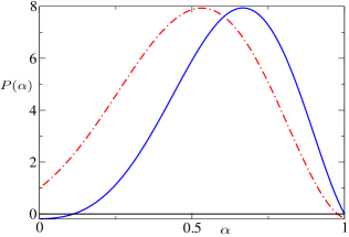
Figure 1: (Color online). Polynomials for symmetric (blue solid line) and antisymmetric (red dashed-dotted line) bound states with the interaction (7), whose roots $\alpha$ characterize the bound states with energy $E=-\alpha-1/\alpha$. The horizontal line corresponds to zero ordinate.

IV Scattering states

After having introduced the first main result of this paper, which deals exclusively with bound states, it is natural to ask about the exact scattering properties of the system. For finite range potentials, the scattering states of the Hamiltonian $\tilde{H}$ are asymptotically plane waves, that is, for $|z|\geq\rho$ we have

$$u_{S}(z) \propto\cos(k|z|+\delta_{S}),$$ (8)

$$u_{A}(z) \propto\operatorname{sgn}(z)\cos(k|z|+\delta_{A}),$$ (9)

where $S$ and $A$ denote, respectively, symmetric and antisymmetric solutions. Their associated eigenenergies are given by the well known tight-binding energy dispersion relation Ashcroft

$$E=-2\cos(k).$$ (10)

However, a general result concerning the phase shifts $\delta_{S}$ and $\delta_{A}$ does not seem feasible, and it is quite cumbersome to obtain them in closed form for long enough ranges. One can, however, calculate the phase shifts (and from them the exact solution at all $z$) numerically by recurrence. To this end, we set $u_{S}(\rho+1)=\cos(k(\rho+1)+\delta_{S})$ and $u_{S}(\rho)=\cos(k\rho+\delta_{S})$ and analogously for antisymmetric solutions, from equations (8) and (9). Then we calculate $u_{S}(-1)$ and $u_{S}(1)$ for symmetric solutions with the help of the Schrödinger equation (4) and solve $u_{S}(-1)=u_{S}(1)$. In the case of antisymmetric solutions, the relevant equation is $u_{A}(0)=0$. We have done so for the example potential of Eq. (7), as is plotted in Fig. 2. There, we clearly observe that the main differences between both phase shifts occur at low quasi-momenta where the symmetric solution is resonant (see Fig. 1); looking at slightly higher quasi-momenta already shows good agreement between both phase shifts. This means that far from $k=0$ fermionization appears rapidly: the large on-site interaction $V(0)$ in (7) acts as a hard-core at high energies, for which the resonance plays no role (it is located at the bottom of the continuum), and therefore the symmetric phase shifts are close to the antisymmetric (“fermionic”). At low quasi-momenta, the resonance obviously dominates the asymptotic behavior of the symmetric scattering states.

In the insets of Fig. 2, we plot the comparison of the phase shifts for the potential in Eq. (7) and a model range-1 potential, whose analytic solution is known MVDP2 . The model potential $W$ is chosen so as to be consistent with Bargmann’s bound HundertmarkSimon , and to be resonant for the lowest-energy symmetric solution. We obtain MVDP2

$$W(1) =-\sum_{z=1}^{10}z^{-3}=-1.19753$$

$$W(0) =-12.125.$$ (11)

The qualitative agreement between the results using $V$ or $W$ for the symmetric eigenstates is manifest in Fig. 2 and, as expected, the differences are most noticeable in the high quasi-momentum regime. For antisymmetric eigenstates the agreement is very good, even quantitatively, until $|k|\simeq\pi/2$. The simplified potential (11) can thus be used as a good approximation for the interaction (7) in the problem of many (spin-polarized) fermions or hard-core bosons on a one dimensional lattice at low energies (around the ground state) and low filling (typically much smaller than half the number of lattice sites). Such a problem can then be solved exactly by means of the Bethe ansatz BetheI .

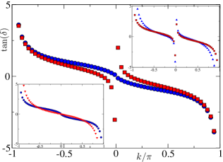
Figure 2: (Color online). The calculated phase shifts ($\tan(\delta)$ with $\delta=\delta_{S}$ or $\delta=\delta_{A}$) for symmetric (blue circles) and antisymmetric (red squares) scattering wave functions, Eqs. (8) and (9), as functions of the relative quasi-momentum $k$, for the potential (7). Left inset: comparison of the symmetric phase shift (blue circles) with the one obtained with a model range-1 potential (red triangles), Eq. (11). Right inset: antisymmetric phase shift (red squares) compared to the result with the model range-1 potential (blue triangles). The axes of the insets have the same meaning as those of the main figure.

V Scattering lengths and zero-energy resonances

V.1 Low-energy scattering

The “low-energy” ($k\to 0,\pi$) scattering properties of the two-body system can be understood via a simple, yet exact, calculation of the scattering lengths. Indeed, the solution of the time-independent Schrödinger equation when $k\to 0$ ($k\to\pi$) has an energy $E=-2$ ($E=+2$), and has the asymptotic ($|z|\geq\rho$) behavior

$$u_{S}(z) =(\mp 1)^{z}\frac{|z|-a_{S}^{\pm}}{\rho-a_{S}^{\pm}}$$ (12)

$$u_{A}(z) =\operatorname{sgn}(z)(\mp 1)^{z}\frac{|z|-a_{A}^{\pm}}{\rho-a_{A}^{\pm}},$$ (13)

where $a_{i}^{-}$ ($a_{i}^{+}$) is the scattering length at $k\to 0$ ($k\to\pi$), $i=S,A$. It must be noted that, in the case of the lattice, there are four different scattering lengths, two for “bosons” (symmetric solutions) and two for spin-polarized “fermions” (antisymmetric solutions). In order to calculate the scattering lengths we proceed as follows : using the recurrence relation from $z=\rho$ by setting $u_{i}(\rho+1)=(\mp 1)^{\rho+1}[1+1/(\rho-a^{\pm})]$, $u_{i}(\rho)=(\mp 1)^{\rho}$ and $E\equiv E_{\pm}=\pm 2$, the scattering lengths for the symmetric states are obtained by solving the equation $(V(0)-E_{\pm})u_{S}(0)-2u_{S}(1)=0$ (see proof of the theorem), while for the antisymmetric states the equation to solve is $u_{A}(0)=0$. It is remarkable that the resulting equations for the scattering lengths as functions of the potential can be cast as linear in $a^{\pm}$, that is, are of the form $s_{0}a^{\pm}+b_{0}=0$ with $s_{0}$ and $b_{0}$ real constants which depend on $V(z)$. In fact, this is an alternative way of defining the four lattice scattering lengths, totally equivalent to the definition $a^{\pm}=-\lim_{k\to\pi,0}\partial_{k}\delta$ PiilMolmerFeshbach , with the advantage of not needing to know the phase shift explicitly. It must be noted at this point that, strictly speaking, scattering lengths are unique of one-dimensional lattices since the radial symmetry is lost in dimensions $d>1$.

As an example, we have calculated $a_{S}^{-}$ for the dipolar potential with a cutoff as $V(0<|z|\leq\rho)=-1/|z|^{3}$, $V(|z|>\rho)=0$, and leaving $V(0)$ as a free parameter. The results are shown in Fig. 3 for a range $\rho=10$, where there is a resonance clearly marked at the point were the scattering length diverges.

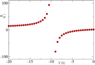
Figure 3: (Color online). Scattering length $a_{S}^{-}$ (see text) as a function of the free parameter $V(0)$, with $V(0<|z|\leq 10)=-1/|z|^{3}$ and $V(|z|>10)=0$.

The divergence of one of the scattering lengths can happen for different values of the total quasi-momentum $K$ footnote3 . In the simplest case of a zero range interaction with $V(0)\equiv U$, the system is known to have no “zero-energy” resonances MVDP1 . For longer ranges, already starting with $\rho=1$ MVDP2 , these resonances can occur. With the method outlined in this work we are able to predict when, for a given range-$\rho$ potential with one or more free parameters $\{V(z_{1}),V(z_{2}),\ldots,V(z_{n})\}$, there is such a resonance. To do so, one sets $u(z\geq\rho)=(\mp 1)^{z}$ and iterates recursively as has been explained, and then solves the resulting equation for symmetric and antisymmetric states, getting a relation among the free parameters of the potential to have a resonance.
We consider again the example of Fig. 3. As we have already noted, the system can admit one resonance at the bottom of the continuum for the symmetric states. From Fig. 3, the approximate location of the resonance can be inferred. However, once the scattering length starts to diverge, an accurate location of the resonance grafically is very hard (if not impossible), especially if the resonance is very sharp as a function of $V(0)$. With our method, we are able to locate the resonance very precisely, obtaining for the example we are dealing with a value of $V(0)=-9.7313$ footnote4 . This is exactly the value chosen in the previous sections to match this resonance.

V.2 Near-resonant bound states

It is well known that the binding energy and size of a near-resonant bound state (NRBS) are closely related to the (large) scattering length $a^{\pm}\lessgtr 0$. On a one dimensional lattice, the relation between the binding energy $E_{b}$ and the scattering length in the effective mass approximation is given by

$$|E_{b}|\approx\frac{\hbar^{2}}{2|m^{\pm}|(a^{\pm})^{2}},$$ (14)

where $m^{\pm}=\mp\hbar^{2}/2$ is the effective mass of the pair with an obvious notation. Note that Eq. (14) is also valid in the context of Feshbach resonances PiilMolmerFeshbach .

When the scattering length is large, the parameter $\alpha$ characterizing a NRBS is close to $\pm 1$ (for $E=-2$ and $E=2$, respectively). By writing $|\alpha|=1-|\xi|$, it is not difficult to show that the size of the bound state, for $\rho\geq 1$, behaves as $\ell^{*}\equiv\langle|z|\rangle\sim 1/(2|\xi|)$ for $|\xi|\ll 1$. Mathematically, one has

$$\lim_{\xi\to 0}|\xi|\ell^{*}=\lim_{\xi\to 0}|\xi|\frac{\langle u|\,|z|\,|u\rangle}{\|u\|^{2}}=\frac{1}{2}.$$ (15)

Since for small $|\xi|$, $|E_{b}|\approx\xi^{2}$, we have that the relation between the size of the NRBS and its associated scattering length is given by

$$\ell^{*}\approx\sqrt{\frac{|m^{\pm}|}{2\hbar^{2}}}|a^{\pm}|=\frac{|a^{\pm}|}{2},$$ (16)

showing that the size of the NRBS grows linearly with the scattering length, as we expected.

V.3 The number of bound states

The scattering lengths are very useful quantities in the sense that knowing their precise values implies knowing the total number of bound states with energies lying below or above the continuum. For this purpose, we use the discrete analog of Sturm oscillation theory Teschl . In simple terms, oscillation theory states that the number of nodes footnote5 of the zero-energy ($E=E_{-}=-2$) symmetric (antisymmetric) solution $u$ of $\tilde{H}u=Eu$ in $\mathbb{Z}_{+}$ is exactly the number of symmetric (antisymmetric) eigenstates below $E_{-}=-2$. Since any state with energy below $E_{-}$ is a bound state, the number of nodes of $u$ is the number of bound states below the continuum. To see how many bound states there are with energies above the continuum, we make use of the transformation $\hat{G}$ of Appendix A, Eq. (19), or, equivalently, count the number of missing nodes.

We apply oscillation theory now to our example with the potential of Eq. (7) leaving again $V(0)$ as a free parameter. We calculate (not shown) the symmetric zero-energy solution for a given scattering length $a_{S}^{-}$ with the methods introduced in this section and see that for $V(0)<-9.7313$ there are two bound states with energies below $E_{-}$ and for $V(0)\geq-9.7313$ there is exactly one bound state below the continuum.

VI A generalization

More general Hamiltonians with exchange operators appear when dealing with the problem of one “free” boson and a bound pair MVDPAS . In such case, the effective particles are distinguishable, there is a hardcore on-site interaction, an effective range-1 potential and a first order exchange term. We assume now that we have the following general one-body Schrödinger operator

$$(H_{\mathrm{ex}}u)(z)= -[u(z+1)+u(z-1)]+V(|z|)u(z)$$

$$+\Omega(|z|)(\hat{P}u)(z),$$ (17)

where $V(0)$ can be finite or infinite and where $\hat{P}$ is the discrete parity operator. We further assume that $\Omega(|z|)$ has a finite range $\rho_{\mathrm{ex}}$ with no on-site exchange, $\Omega(0)=0$, since it can be included in $V(0)$.

Obviously $[\hat{P},H_{\mathrm{ex}}]=0$, and therefore we can look for symmetric and antisymmetric solutions. However, the Hamiltonian does not commute with the exchange operator $\Omega\hat{P}$. With the parity as a good quantum number it is straightforward to generalize the theorem of Section III to include exchange. To see this, take $\rho_{M}\equiv\max(\rho,\rho_{\mathrm{ex}})$. If $u(z)$ is symmetric, the exchange shifts the potential to $V(|z|)+\Omega(|z|)$, while if $u(z)$ is antisymmetric it shifts the potential to $V(|z|)-\Omega(|z|)$. Therefore, obtaining the bound states of $H_{\mathrm{ex}}$ reduces again to a polynomial equation of degree $2\rho_{M}\pm 1$, and all the results of our theorem apply by changing $\rho$ by $\rho_{M}$ and $V$ by $V\pm\Omega$. However, it is no longer true that a hardcore condition $|V(0)|\to\infty$ maps “bosons” onto “fermions” (symmetric onto antisymmetric solutions). Indeed, the non-trivial dependence of $H_{\mathrm{ex}}$ on the parity of the eigenstates makes it possible to have states above as well as below its continuum even if $V$ and $\Omega$ have both the same definite sign. This is the fact that makes $H_{\mathrm{ex}}$ violate the hypotheses of the BFMT Girardeau , and it explains the appearance of exotic three-body bound states on a 1D lattice MVDPAS .

VII Conclusions

In this paper, we have shown how the exact wave functions and energies of any bound state of two particles on a one-dimensional tight-binding lattice can be calculated by solving a polynomial equation whose order increases slowly with increasing range of the two-body interaction potential, which can also include parity-dependent terms, such as effective particle exchange. We have shown that the calculation of the exact scattering states is possible, and simple. We have also shown how the zero-energy resonances associated with the entry or exit of a bound state can be trivially and exactly located, and related the scattering lengths to the number of bound states above or below the continuum by making reference to the discrete version of Sturm theory.

There are, on the other hand, many open problems in the physics of few particles on a lattice. At the two-body level, there is still no general prescription for the calculation of bound and scattering states on two- and three-dimensional lattices with arbitrary finite range interactions. For the three-body case, the Efimov effect Efimov , which was shown to appear on a three-dimensional (3D) simple cubic lattice RevMattis , has not been quantitatively examined yet; the lattice Efimov effect should depend largely on the total quasi-momentum of the system and, moreover, there should appear new kinds of exotic three-body bound states in 3D with no analog in continuous space, as has been shown to be the case in 1D MVDPAS . It would also be very interesting to explore few-body effects in other lattice geometries.

Appendix A Equivalence between repulsive and attractive potentials

We state a general result for an $N$-body system on a hypercubic lattice in any dimension which, although being usually implicitly assumed, is useful and important to keep in mind, specially when dealing with purely attractive or repulsive two-body interactions.

Let $H$ be the following second-quantized Hamiltonian

$$H=-J\sum_{\langle\mathbf{m},\mathbf{n}\rangle}\hat{a}^{\dagger}_{\mathbf{m}}\hat{a}_{\mathbf{n}}+\hat{F}(\{\hat{N}\}),$$ (18)

where $J$ is the single-particle tunneling rate, $\langle\mathbf{m},\mathbf{n}\rangle$ denotes that the sum runs only through nearest neighbors, $\hat{a}^{\dagger}_{\mathbf{n}}$ ($\hat{a}_{\mathbf{n}}$) is the creation (annihilation) operator of a single particle (boson or fermion) at site $\mathbf{n}$ and where $\hat{F}$ is an arbitrary analytic function of the number operators at each site $\mathbf{n}$, $\hat{N}_{\mathbf{n}}\equiv\hat{a}^{\dagger}_{\mathbf{n}}\hat{a}_{\mathbf{n}}$.
If $\mathbf{n}\equiv(n_{1},n_{2},\ldots,n_{d})$ is a point of a $d$-dimensional hypercubic lattice, we define the unitary operation $\hat{G}$ so that $\hat{G}=\hat{G}^{\dagger}=\hat{G}^{-1}$, with the actions

$$\hat{G}\hat{a}^{\dagger}_{\mathbf{n}}=(-1)^{\sum_{s=1}^{d}n_{s}}\hat{a}^{\dagger}_{\mathbf{n}}.$$ (19)

We easily see that $H-2\hat{F}=-\hat{G}H\hat{G}^{-1}$ is unitarily equivalent to $-H$. This implies that the spectrum of a Hamiltonian containing the potentials included in $\hat{F}$ is obtained by changing the sign of every point in the spectrum of the corresponding Hamiltonian having $\hat{F}$ replaced by $-\hat{F}$. In the case of $\hat{F}$ containing purely repulsive (or attractive) two-body interactions, this result implies the formal equivalence between attractive and repulsive potentials.

References

- (1) N.J. Ashcroft and and N.D. Mermin, Solid State Physics (International Thomson Publishing, New York, 1976).
- (2) J. Hubbard, Proc. Roy. Soc. A 276 238 (1963).
- (3) M.P.A. Fisher, P.B. Weichman, G. Grinstein, and D.S. Fisher, Phys. Rev. B 40, 546 (1989).
- (4) D. Jaksch et al., Phys. Rev. Lett. 81, 3108 (1998).
- (5) O. Morsch and M. Oberthaler, Rev. Mod. Phys. 78, 179 (2006); I. Bloch, J. Dalibard, and W. Zwerger, Rev. Mod. Phys. 80, 885 (2008); M. Lewenstein et al., Adv. Phys. 56, 243 (2007).
- (6) M. Greiner et. al., Nature 415, 39 (2002).
- (7) K. Winkler et al., Nature 441, 853 (2006).
- (8) R. Piil and K. Mølmer, Phys. Rev. A 76, 023607 (2007).
- (9) M. Valiente and D. Petrosyan, J. Phys. B 41, 161002 (2008).
- (10) M. Valiente and D. Petrosyan, J. Phys. B 42, 121001 (2009).
- (11) M. Valiente, D. Petrosyan and A. Saenz, Phys. Rev. A 81, 011601(R) (2010).
- (12) C. Weiss and H.-P. Breuer, Phys. Rev. A 79, 023608 (2009).
- (13) L. Jin, B. Chen and Z. Song, Phys. Rev. A 79, 032108 (2009).
- (14) R. T. Piil, N. Nygaard, and K. Mølmer, Phys. Rev. A 78, 033611 (2008).
- (15) D. C. Mattis, Rev. Mod. Phys. 58, 2, 361 (1986).
- (16) In continuous space this is equivalent to particles with different masses.
- (17) J.-P. Martikainen, Phys. Rev. A 78, 035602 (2008).
- (18) M.D. Girardeau, J. Math. Phys. 1, 516 (1960).
- (19) D. Petrosyan et al., Phys. Rev. A 76, 033606 (2007).
- (20) D. Damanik, D. Hundertmark, R. Killip and B. Simon, Commun. Math. Phys. 238, 545 (2003).
- (21) G. Teschl, Jacobi operators and completely integrable nonlinear lattices (Mathematical surveys and monographs, American Mathematical Society, 2000).
- (22) C. Menotti, C. Trefzger and M. Lewenstein, Phys. Rev. Lett. 98, 235301 (2007).
- (23) C. Trefzger, C. Menotti and M. Lewenstein, Phys. Rev. A 78, 043604 (2008).
- (24) Th. Lahaye, C. Menotti, L. Santos, M. Lewenstein and T. Pfau, Rep. Prog. Phys. 72, 126401 (2009).
- (25) Note that since for all , there can be no roots for .
- (26) D. Hundertmark and B. Simon, J. Approx. Theory 118, 106 (2002).
- (27) M. Karbach and G. Müller, Comp. in Phys. 11, 36 (1997).
- (28) N. Nygaard, R. Piil and K. Mølmer, Phys. Rev. A 78, 023617 (2008).
- (29) Note that we have normalized the Hamiltonian as .
- (30) If the calculation is implemented with a symbolic package, the value of at which the resonance occurs can be calculated exactly (with no machine precission limit). In our example, is a rational number whose (large) numerator and denominator can be calculated exactly this way.
- (31) On the lattice, a function is said to have a node between and iff .
- (32) V.N. Efimov, Phys. Lett. B 33, 563 (1970).