Visualizing quantum entanglement and the EPR -paradox during the photodissociation of a diatomic molecule using two ultrashort laser pulses

Abstract

We investigate theoretically the dissociative ionization of a ${\rm H_{2}^{+}}$ molecule using two ultrashort laser (pump-probe) pulses. The pump pulse prepares a dissociating nuclear wave packet on an ungerade surface of ${\rm H_{2}^{+}}$ . Next, an UV (or XUV) probe pulse ionizes this dissociating state at large (R = 20 - 100 bohr) internuclear distance. We calculate the momenta distributions of protons and photoelectrons which show a (two-slit-like) interference structure. A general, simple interference formula is obtained which depends on the electron and protons momenta, as well as on the pump-probe delay on the pulses durations and polarizations. This interference can be interpreted as visualization of an electron state delocalized over the two-centres. This state is an entangled state of a hydrogen atom with a momentum $\vec{p}$ and a proton with an opposite momentum $-\vec{p}$ dissociating on the ungerade surface of ${\rm H_{2}^{+}}$ . This pump-probe scheme can be used to reveal the nonlocality of the electron which intuitively should be localized on just one of the protons separated by the distance R much larger than the atomic Bohr orbit.

I Introduction

Recently, due to the extraordinary increase of research activities in quantum information and quantum cryptography there is a growing interest in various quantum intriguing phenomena originating back to the famous Einstein-Podolski-Rosen (EPR) paradox Einstein1935 formulated in 1935. This paradox is related to the phenomenon of quantum entanglement Ekert2009 and to the non-local character of quantum mechanics Dunningham07 or to the problem of local realism versus the completness of quantum mechanism. A most recent comprehensive review of various aspects of the EPR paradox can be found in Reid2009 . So far nearly all experimental evidence for entanglement is related to the measurement of correlated photon pairs obtained in a process called ”parametric down-conversion Aspelmeyer2008 . In such processes a photon from a laser beam gets absorbed by an atom which subsequently emits two ”polarization entangled” photons. The entanglement phenomenon should in principle also appear in various break-up processes involving slower (massive) fragments than photons, e.g. in various disintegration processes such as photoionization and photodissociation, as suggested in Fedorov2006 ; Fedorov2004 ; Fry1995 ; Gneiting2008 ; Opatrny2001 ; Savage2007 . So far, there exist very few experimental results demonstrating the entanglement in such slower processes and involving massive particles which are much better localized in space than massless photons Reid2009 .

In this letter we investigate theoretically an experimental scheme based on recent advances in the ultrashort laser technologies which allow to shape laser pulses in femtosecond or even sub-femtosecond (attosecond) time scales Krausz2009 ; Vrakking2009 . Thus these technologies allow to image the evolution in time of correlated electron-nuclear wave function. This can be achieved by initiating the dissociation process using an ultrashort pump pulse and allowing the dissociating fragments to separate and be far apart. Next, this system can be probed via a photoionization process using a probe pulse having a well defined phase relative to the pump pulse, and consequently in phase with the dissociating system. In general the photoelectron spectra will exhibit a two-centre interference, sometimes called a Fano interference since it was predicted by Cohen and Fano in 1967 Cohen1966 . Their calculations showed that when a molecule is photoionized via absorption of one photon the photelectron spectra in diatomic molecules are modulated by an interference factor

$$\bar{\chi}=1\pm{\sin(|\vec{p}_{e}|R_{eq})\over|\vec{p}_{e}|R_{eq}}\;\;,$$ (1)

where $\vec{p}_{e}$ is the electron momentum and $R_{eq}$ is the equilibrium internuclear distance and the sign depends on the parity of the molecular electronic wave function; (+) for a gerade and (-) for an ungerade electronic state. We show that if the Fano interference is observed in dissociating diatomic molecule at large internuclear separation it may become an important tool for visualizing peculiarities of quantum mechanics related to entanglement and to the nonlocal character of the electron which (intuitively) should localize on a single heavy (1836.15 times heavier than the electron) centre, during the dissociation process, due to localization via Coulomb attractive force. Note that a quantum state describing a localized electron on a specific proton accompanying another distant proton would not lead to the two-centre Fano interference in the photoelectron spectrum. This interference is a result of the unique gerade or ungerade symmetry of the electronic molecular wave function before the photoionization takes place. Since the molecular Hamiltonian has also this symmetry we conclude that the state before the turn-on of the probe pulse should preserve the symmetry of the dissociating state prepared by a pump pulse. In other words, quantum dissociating state is not a simple product of the hydrogen and proton states but is a coherent superposition of the possible ”simultaneous presence” of the electron on both well separated protons. Thus in this specific dissociation process we face clearly the conflict with local realism: in any deterministic theory the simultaneous presence of the electron on two heavy well separated protons should not occur, and, consequently the observation of Fano interference pattern is in conflict with local realism in a similar way as the experimental violation Bell inequalities is Reid2009 .

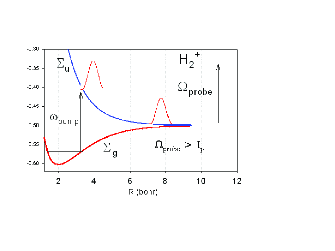
Figure 1: Illustration of the proposed pump-probe experimental scheme. Two lowest electronic surfaces $\Sigma_{g}$ and $\Sigma_{u}$ of ${\rm H_{2}^{+}}$ are shown. The pump pulse prepares the nuclear wave packet sliding on the upper ungerade surface $\Sigma_{u}$. After the turn-off of the pump pulse this wave packet evolves as free system until it is photoionize at large internuclear distance R.

More specifically, we consider a pump-probe excitation scheme Krausz2009 ; Vrakking2009 in which a pump laser pulse prepares a dissociating nuclear wave packet on an ungerade (repulsive) surface of a ${\rm H_{2}^{+}}$ molecule. Next (20-200 fs later, after the pump pulse is turned-off), a UV (or XUV) probe pulse ionizes this dissociating (H-atom + proton) state at large (R = 20 - 150 bohr) internuclear distance, as illustrated in Fig.1 and also described in Vrakking2009 . We show that coincidence measurement of the electron and proton spectra reveal a very special, counter-intuitive nature of the quantum dissociation process. It can be assumed that after the turn-off of the pump pulse the motion on the ungerade surface of ${\rm H_{2}^{+}}$ is adiabatic. Consequently, because the antisymmetric (or symmetric if disociation occurs on a gerade electronic state) character of the electronic wave function the quantum state of the dissociating system is very distinct from a state of a free proton and a free hydrogen atom Bykov2003 which for instance occurs in proton-hydrogen scattering. Thus quantum mechanics predicts that even at large internuclear distance the electron can be well localized in two places, i.e. it can form a hydrogen atom on two well separated protons which seems counter-intuitive. Note that in our scheme electron localization occurs due to the Coulomb attraction from two protons. Suppose that we have measured the hydrogen atom at the right hand side along the laser polarization vector, as shown in Fig.2 . Already at relatively small internuclear distance R=10 bohr shown in Fig.2 the electron is very well localize on each centre. Thus we infer (using the charge conservation principle) that the opposite detector (at left-hand side in Fig.2) at the internuclear separation larger that R=60 bohr will measure with a certitude a proton. This situation resembles a variant of the EPR paradox based on the disintegrating system of the two, spin one-half particles, originating from their initial singlet state Sakurai1985 in which by measuring a spin up by one detector we infer what was the spin projection measured by the opposite detector.

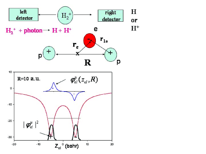
Figure 2: The upper part shows schematically the first stage of the proposed experimental scheme in the case when only the laser pump pulse is used. This pulse dissociates the ${\rm H_{2}^{+}}$ molecule. Two opposing detectors are measuring the H-atom or the H⁺ ion . These measurements resemble the case of the EPR paradox in which the spin projections are measured in the disintegration of the two spin one-half particles from the initial single spin state. We also illustrate the definition of the Jacobi coordinates for the p-p-e system used in our calculations. The lower part show the two-centre Coulomb potential, the ungerade electronic wave function $\varphi_{el}^{u}$ and the corresponding probability density as function of the electron coordinate $z_{el}$ at fixed intenruclear distance R=10 bohr.

Suppose now that instead of measuring directly the H-atom in the above experiment we use a probe UV pulse which photoionizes the molecule and the two-centre Fano interference pattern is observed in the photoionization signal. Simple perturbative calculations using a plane wave approximation for the final electrons state Cohen1966 ; Yudin2006 predict that at fixed internuclear vector $\vec{R}$ the molecular photoelectron signal is modulated via interference factors $\sin^{2}(\vec{p}_{e}\cdot\vec{R}/2)$ or $\cos^{2}(\vec{p}_{e}\cdot\vec{R}/2)$. Just the fact that we observe such an interference at large $|\vec{R}|$ would be a witness of the two following interesting quantum phenomena. First, in the proposed experiment the probe pulse will monitor an entangled state of two particles: the hydrogen atom and the proton, represented by the state $|H,\vec{p}>$ times and the $H^{+}$ (i,e, proton) flying in an opposite direction represented by a ket $|H^{+},-\vec{p}>$. The dissociating state is not a simple product of these basis states but because of the electron symmetry of the state dissociating on a single electron surface we must add to the product: $|H,\vec{p}>|H^{+},-\vec{p}>$ the product $|H,-\vec{p}>|H^{+},\vec{p}>$ and integrate over the relative momentum $\vec{p}$ weighed with the momentum distribution of the dissociating wave packet. If a two-centre interference pattern is observed in the photoelectron signal this means that we observe an entangled state, since a simple product of these states cannot yield a two centre interference pattern. Second, any local hidden variable theory would predict the electron position with respect to one of the protons is well defined within the Bohr radius. Thus when the interference pattern is observed in the photoelectron spectrum this means that the electron is well localized simultaneously on both well separated protons before we photoionized this quantum system. This is a very unusual situation since the tunneling time from one centre to another is extremely large even at the relatively small internuclear separation R=60 bohr: t_tunnel= 2.4 years Bykov2003 . Moreover, if we interpret the integral of e$|\psi|^{2}$ over half-space as a charge present around a specific proton one concludes that a fractional charge e/2 is well localized around one centre Bykov2006 . Thus one may argue that the observation of the Fano two-centre interference is a witness for the simultaneous presence of a charge e/2 on each centre. Clearly, this simple 3-body system with the electron and two well separated protons represents an interesting quantum mystery related to the formation of a hydrogen atom during the dissociation process and is certainly worth further experimental and theoretical investigation.

In our theoretical description of the above mentioned pump-probe scheme (dissociation followed by photoionization), we do not calculate the dynamics of the first step in which an ultrashort UV pump pulse photodissociates (via an absorption of one photon) the ${\rm H_{2}^{+}}$ molecule and it thus prepares a nuclear wave packet moving on the molecular ungerade surface. We assume that this wave packet has the Gaussian shape right after the pump pulse is turned off, centres at $R$=$R_{0}$=12 bohr, at t=0, and it next evolves as a free system (field-free) on the $\Sigma_{u}$ surface up to R=60-120 bohr when an ultrashort UV pump laser pulse is turned-on and it photoionizes this dissociating packet also via an one photon process. The photoionization probability distributions of the momenta of the electron and the protons are calculated using first order perturbation theory in 3-D (3-D for both electron and nuclear degreees of freedom). A plane wave approximation is used for the final state of protons and a ”modified-plane-wave” approximation for the electron (see next Section for the details). Note that to the best of our knowledge, all theoretical work related to Fano interference has been so far done using frozen nuclei at fixed equilibrium internulear distance $|\vec{R}_{eq}|$. We believe that our study is the first dynamical investigation of Fano interference in the photoelectron spectrum originating from dissociating molecules at large internuclear separations. It includes full 3-D electron-nuclear dynamics. Note, that so far approaches based on solving time-dependent Schrödinger equation for ${\rm H_{2}^{+}}$ are based on the models with reduced dimensionality Bandrauk2009 ; Bandrauk1999 .

II Perturbative calculations of dissociative-ionization

We use Jacobi coordinates for the electron and two protons (separated by a vector $\vec{R}$) in which the electron position vector $\vec{r}_{e}$ originates in the centre of mass of two protons, see Fig.2. In these coordinates the Hamiltonian of ${\rm H_{2}^{+}}$ has the following form Hiskes1961 : (in atomic units, $\hbar=m_{e}=e$=1)

$$\hat{H}_{0}=-{1\over 2m^{\prime}_{e}}\Delta_{\vec{r}_{e}}-{1\over 2\mu}\Delta_{\vec{R}}+V_{C}(\vec{r}_{e},\vec{R})\;,$$ (2)

where

$$m^{\prime}_{e}=\;{2m_{p}m_{e}\over 2m_{p}+m_{e}}\;,\mu=m_{p}/2$$

are the electron - two proton reduced mass and the proton-proton reduced mass, respectively,

$$V_{C}(\vec{r}_{e},\vec{R})\;=\;{-1\over|\vec{r}_{e}-\vec{R}/2|}\;+\;{-1\over|\vec{r}_{e}+\vec{R}/2|}\;+\;{1\over|\vec{R}|}$$ (3)

is the total Coulomb interaction between protons and the electron and $m_{e}$ and $m_{p}$ are the electron and proton masses. The total Hamiltonian is $\hat{H}=\hat{H}_{0}+\hat{V}_{int}$ where

$$\hat{V}_{int}=-i{\kappa\over m^{\prime}_{e}c}\vec{A}(t)\nabla_{\vec{r}_{e}},$$ (4)

where

$$\kappa\;=\;1+{m_{e}\over{2m_{p}+m_{e}}}\;\;.$$

$V_{int}$ describes the interaction of ${\rm H_{2}^{+}}$ with a UV laser probe field via its vector potential. Since we use a weak intensity probe pulse and the pulse frequency is larger than ionization potential of ${\rm H_{2}^{+}}$ we may use the perturbation theory for calculation of the photoionization probability of the dissociating wave packet (prepared by the pump pulse) using the transition amplitude:

$$A_{fi}=-i\int_{-\infty}^{\infty}dt\langle\psi_{f}|e^{i\hat{H}_{0}t}V_{int}e^{-i\hat{H}_{0}t}|\psi_{in}(t)\rangle$$ (5)

We first recall the result for fixed nuclei at $\vec{R}$. Using for the electron initial state

$$\varphi_{el}^{g/u}(\vec{r}_{e},\vec{R})=\frac{1}{\sqrt{2}}\left[\psi_{H}(\vec{r}_{e}+\vec{R}/2)\pm\psi_{H}(\vec{r}_{e}-\vec{R}/2)\right]$$ (6)

where $\psi_{H}$ is the hydrogen 1s wave function (sign ($\pm$) is used for the electronic gerade on ungerade state), and using the plane wave for the final electron state:

$$\psi_{f}=(2\pi)^{-3/2}\exp(i\vec{p}_{e}\cdot\vec{r}_{e})$$ (7)

we get from eq. (5) (just by choosing the integration coordinates local to each centre) that

$$|A_{fi}^{fix}|^{2}\;\sim\;\left[1\pm\cos(\vec{p}_{e}\cdot\vec{R})\right]|A_{H}(\vec{p}_{e})|^{2}$$ (8)

where $A_{H}(\vec{p}_{e})$ is the atomic photoionziation amplitude given in Yudin2006 . Thus if ionization occurs from the ungerade surface the molecular ionization probability is modulated via a $\sin^{2}(\vec{p}_{e}\cdot\vec{R}/2)$ factor. If the molecule is not initially aligned, and if protons momenta are not measured, we need to integrate over the direction of $\vec{R}$ which leads to the $\bar{\chi}$ factor given in eq.(1). To include the nuclear motion in eq.(5) we use the plane wave approximation for the final state for both the electron and for the relative motion of protons:

$$\psi_{f}=(2\pi)^{-3}\exp(i\vec{p}_{N}\cdot\vec{R})\exp(i\vec{p}_{e}\cdot\vec{r}_{e}).$$ (9)

We will isolate from this expression the electronic atomic photoionization amplitude $A_{H}(\vec{p}_{e})$ in which we will use the exact expression for an atomic amplitude, i.e. in which exact Coulomb wave for the individual centre is included (but the influence of the neighboring centre is neglected which is a reasonable approximation for the case of very large R we are interested in). This explains the term ”modified-plane-wave” approximation used in the introduction. Regarding the plane wave approximation for the nuclei we think that it is justified for photoionization occurring at very large internuclear distances. We are interested in R’s as large as $R>60$ bohr at which Coulomb repulsion should be negligible with respect to the kinetic energy of the the dissociating ${\rm H_{2}^{+}}$ , i.e. when

$$\frac{p_{0}^{2}}{2\mu}\gg\frac{e^{2}}{R_{0}+p_{0}t_{c}/\mu}\;\;$$ (10)

where $R_{0}$ is the position of the the centre of the dissociating wave packet with the momentum $p_{0}$ at t=0 when the pump pulse is turned off and $t_{c}$ is the time at which the amplitude of the probe pulse is at maximum. At this time the wave packet reaches the distance $R_{0}+p_{0}t_{c}/\mu\;$. These plane wave approximations allow us to get a simple analytic expression for the amplitude $A_{fi}(\vec{p}_{e},\vec{p}_{N},\tau,\Delta R,t_{c})$. Using the Coulomb waves in the final state leads to much more complicated formulas involving some numerical integration.

As the initial state we take the Born-Oppenheimer solution (we consider an improvement to this approximation in the appendix) as a product of the ungerade electronic function (6) and the superposition of nuclear plane waves $\exp(i\vec{p}\cdot\vec{R})$ :

$$\psi_{in}(\vec{r}_{e},\vec{R},R_{0})=\varphi_{el}^{u}(\vec{r}_{e},\vec{R})\int d^{3}p\;\varphi_{N}(\vec{p},R_{0})\exp(i\vec{p}\cdot\vec{R})$$ (11)

where $\varphi_{N}(\vec{p},R_{0})$ is the initial distribution of the momenta in the dissociating nuclear wave packet. It should be adjusted to the shape of the wave packet prepared by the pump pulse which we suppose is short and in the amplitude (5) we assume the free evolution of the ${\rm H_{2}^{+}}$ wave packet between the turn-off the pump pulse at t=0 and the turn-on of the probe pulse. We derive next the analytic formula for photoionization valid for any shape of $\varphi_{N}(\vec{p},R_{0})$. Its specific shape will be chosen for illustrating graphically our results. In order to perform analytically the time integral in (5) we need a specific shape of the vector potential $\vec{A}(t)$ of the laser field. We assume it has a Gaussian form:

$$\vec{A}(t)=\frac{\vec{e}_{probe}}{2}A_{0}\exp\left[-\frac{(t-t_{c})^{2}}{2\tau^{2}}\right]\exp(-i\Omega_{probe}t)+C.C.\;\;$$ (12)

where $A_{0}$, $\vec{e}_{probe}$, $\Omega_{probe}$, $\tau$ are the UV probe pulse amplitude, polarization, its central frequency and duration. Pulse duration $\tau$ is related to the commonly used FWHM duration via relation $\tau_{FWHM}=2\sqrt{\ln(2)}\tau$. We recall that thus defined FWHM means full width at half maximum of the laser intensity time profile, not the FWHM of the envelope of the laser field. $t_{c}$ is the time at which the probe pulse has maximum and at the same time $t_{c}$ is also a measure the time delay between the probe and the pump pulse since we have chosen t=0 as time when the pump pulse is turned off and the centre of the nuclear packet is at $R=R_{0}$.

After integrating the time t and the electronic coordinate $\vec{r}_{e}$, in the formula (5) we get :

$$A_{fi}=N_{1}A_{H}\left(\vec{p}_{e}\right)\int d^{3}p\;a(\vec{p})\;\int d^{3}R\exp\left(i\vec{p}\cdot\vec{R}-i\vec{p}_{N}\cdot\vec{R}\right)\left(e^{i\vec{p}_{e}\cdot\vec{R}/2}-e^{-i\vec{p}_{e}\cdot\vec{R}/2}\right)$$ (13)

where

$$a(\vec{p})=\exp[if(\vec{p})t_{c}-\tau^{2}f(\vec{p})/2]\varphi_{N}(\vec{p},R_{0})\;\;,$$ (14)

$$f(\vec{p})={\vec{p}\;^{2}_{e}\over 2m^{\prime}_{e}}+{\vec{p}\;^{2}_{N}\over 2\mu}+I_{p}-\Omega_{probe}-{\vec{p}\;^{2}\over 2\mu}\;\;,N_{1}={\kappa A_{0}\tau\over 2\pi 2^{3/2}m^{\prime}_{e}c}\;,\;$$ (15)

$$A_{H}(\vec{p}_{e})=A_{1s}(\vec{p}_{e})=2^{3/2}\frac{(\vec{e}\cdot\vec{p}_{e})(1-i\nu)}{\pi(1+\vec{p}_{e}^{2})^{2}}\exp\left[-2\nu\arctan(p_{e})\right]N_{\nu}^{*}\;,$$ (16)

$$\nu={1\over p_{e}}\;\;,\;\;N_{\nu}=\exp(\pi\nu/2)\Gamma(1+i\nu)\;\;\;.$$

Integration over the $\vec{R}$ coordinate yields two Dirac delta functions for momentum conservation. Thus we get for the dissociative-ionization amplitude

$$A_{fi}=N_{1}(2\pi)^{3}A_{H}(\vec{p}_{e})\int d^{3}p\;a(\vec{p})\;[(\delta(\vec{p}-\vec{p}_{N}+\vec{p}_{e}/2)-\delta(\vec{p}-\vec{p}_{N}-\vec{p}_{e}/2)]$$ (17)

Integration over the nuclear momenta $\vec{p}$ yields the final probability amplitude for dissociative-ionization

$$A_{fi}(\vec{p}_{e},\vec{p}_{N},\tau,\Delta R,t_{c})=N_{2}A_{H}(\vec{p}_{e})\left[a(\vec{p}_{-})-a(\vec{p}_{+})\right]$$ (18)

where $a(\vec{p})$ is defined in (14),

$$N_{2}=(2\pi)^{3}N_{1}={\kappa A_{0}(2\pi)^{2}\tau\over 2^{3/2}m^{\prime}_{e}c}\;\;,$$

and

$$\vec{p}_{\pm}=\vec{p}_{N}\pm\vec{p}_{e}/2\;\;.$$ (19)

The shifted momentum in the last equation is related to the recoil received by each proton from the electron: the final relative momentum is either $\vec{p}_{+}$ or $\vec{p}_{-}$.

Eq.(18) provides a general expression for the momenta distributions of protons and of the electron valid for any initial distribution of momenta $\varphi_{N}(\vec{p},R_{0})$ of a dissociating wave packet. However, in order to investigate in detail Fano two-centre interference effect we need to specify the initial momentum distribution in the wave packet prepared by the pump pulse. We suppose that the ${\rm H_{2}^{+}}$ molecule was initially in the vibrational v=0, J=0 of the gerade bound state, where J is the initial angular momentum quantum number of the molecule. Thus the nuclear wave packet, after absorption of one photon, will be in the J=1 rotational state on the ungerade $\Sigma_{u}$ surface of ${\rm H_{2}^{+}}$ . We assume that it has the form:

$$\varphi_{N}\left(\vec{p},R_{0}\right)=C_{N}\frac{\cos\theta_{p}}{p}\exp\left(-\frac{\Delta R^{2}}{2}(p-p_{0})^{2}\right)\exp\left[i(p_{0}-p)R_{0}\right]$$ (20)

where $\cos\theta_{p}=\vec{p}\cdot\vec{e}_{pump}/|\vec{p}|$ and $\theta_{p}$ is angle between the nuclear relative momentum $\vec{p}$ and the pump pulse polarization. The nuclear wave packet is at $R=R_{0}$ at $t=0$, the probe has maximum at $t=t_{c}$. This is a free Gaussian wave packet (in the radial variable $p=|\vec{p}|$ ) sliding on the electronic surface $\Sigma_{u}$ (its electronic wave function $\varphi_{el}^{u}$ is given in (6) with the angular momentum J=1. The central radial momentum of the wave packet is $p_{0}$ and its spatial width is $\Delta R$. In order to study the two-centre interference effect it is convenient to rewrite the probability of ionization in the following form (in this form the interference appears through the cross term C):

$$|A_{fi}(\vec{p}_{e},\vec{p}_{N},\tau,\Delta R,t_{c})|^{2}=|A_{H}(\vec{p}_{e})|^{2}\left[|a(\vec{p}_{-}|^{2}+|a(\vec{p}_{-}|^{2}+C({p}_{+},{p}_{-},t_{c})\right]$$ (21)

where

$$|a(\vec{p})|=C_{N}\exp\left(-f^{2}(\vec{p})\frac{\tau^{2}}{2}-\frac{\Delta R^{2}}{2}(p-p_{0})\right)|\vec{p}\cdot\vec{e}|\;/|\vec{p}|^{2},\;\;,$$ (22)

$$C({p}_{+},{p}_{-},t_{c})=2|a(\vec{p}_{+})|\;|a(\vec{p}_{-})|\cos(\Phi(t_{c}))\;\;,$$ (23)

$$\Phi(t_{c},\vec{p}_{e}\;,\vec{p}_{N})=(|\vec{p}_{+}|-|\vec{p}_{-}|)R_{0}+\left[f(\vec{p}_{-})|-f(\vec{p}_{+})\right]t_{c}=(|\vec{p}_{+}|-|\vec{p}_{-}|)R_{0}+{|\vec{p}_{+}|^{2}-|\vec{p}_{-}|^{2}\over 2\mu}\;t_{c}\;.$$ (24)

After the use of eq.(19) the phase $\Phi$ becomes

$$\Phi(t_{c},\vec{p}_{e},\vec{p}_{N})=(|\vec{p}_{+}|-|\vec{p}_{-}|)\;R_{0}+\vec{p}_{e}\cdot{\vec{p}_{N}\over\mu}\;t_{c}\;\;.$$ (25)

This is an important result since after comparing eq.(25) with the phase corresponding to static result eq.(8) we conclude that by measuring the relative nuclear momentum $p_{N}$ and the delay time $t_{c}$ we are fixing the increment of the internuclear separation $\vec{R}$ during the time interval $t_{c}$, i.e. this increment is simply: $\vec{v}_{N}t_{c}$ where $\vec{v}_{N}=\vec{p}_{N}\;/\;\mu$ is the relative velocity of protons. We can simplify more equation (25) in the case of the nuclear momentum larger than the electron momentum, i.e. if the inequality $p_{e}\;<<\;p_{N}$ holds we get:

$$|\vec{p}_{\pm}|=\sqrt{p_{N}^{2}\pm\vec{p}_{e}\cdot\vec{p}_{N}+p_{e}^{2}/4}\simeq p_{N}\pm\vec{p}_{e}\cdot{\vec{p}_{N}\over 2p_{N}}\;=\;p_{N}\pm p_{e}\cos(\theta_{pe})\;/2;\;.$$ (26)

Thus the phase (25) on which the interference relies simplifies to:

$$\Phi(t_{c},\vec{p}_{N}))\simeq\vec{p}_{e}\cdot\vec{R}_{N}(t_{c},\vec{p}_{N})\;\;,$$ (27)

where

$$\vec{R}_{N}(t_{c},\vec{p}_{N})\simeq R_{0}{\vec{p}_{N}\over|\vec{p}_{N}|}+{\vec{p}_{N}t_{c}\over\mu}\;\;.$$ (28)

We will also use later the absolute value of the vector $\vec{R}_{N}$:

$$R_{N}(t_{c},p_{N})=|\vec{R}_{N}(t_{c},\vec{p}_{N})|\simeq R_{0}+{p_{N}t_{c}\over\mu}\;\;.$$ (29)

Clearly, we see from the last equations that, as in the case of static result (8) the interference term $C({p}_{+},{p}_{-},t_{c})$ is modulated via the term $\cos\left[R_{N}(t_{c},p_{N})p_{e}\cos(\theta_{ep})\right]\;,$ where $\theta_{ep}$ is the angle between the electron momentum and relative nuclear momentum $\vec{p}_{N}$. This relation can be used for imaging the nuclear motion as suggested in Vrakking2009 : if we measure the ionization signal for a series of time delays $t_{c}$ and follow the change of a specific minimum in the spectrum, we can thus deduce the molecular trajectory from the relation $2n\pi/p_{e}cos(\theta_{ep})$, where n is an integer corresponding to a specific minimum.

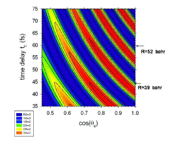
Figure 3: Ionization probability calculated using eqs.(21)-(24) for the case when the polarizations of the pump and probe pulses are parallel and the nuclear relative momentum $\vec{p}_{N}$ is also parallel to both polarizations. We used: $\lambda_{probe}$=60 nm, $p_{N}=p_{0}=$14.8 a.u.,$p_{e}$=0.72 a.u., $\Delta R$= 3.0 bohr, $R_{0}$=12.0 bohr and the pump pulse duration $\tau_{FHWM}$=2.4 fs.

If furthermore, the width of the momentum distribution ${1\over\Delta R}$ is sufficiently large compared to the electron momentum $p_{e}$, i.e. $p_{e}<{1\over\Delta R}$, we may expect that the following approximations are valid for $p_{N}$ values close to the central value $p_{0}$ of the momentum distributions defined via (20):

$$|a(\vec{p}_{-}|\simeq|a(\vec{p}_{+}|)\;\simeq|a(\vec{p}_{N}|)\;\;,$$ (30)

we get

$$|A_{fi}|^{2}\sim|A_{H}(\vec{p}_{e})|^{2}\sin^{2}\left(\vec{p}_{e}\cdot\frac{\vec{p}_{N}}{|\vec{p}_{N}|}R_{N}(t_{c},|\vec{p}_{N}|)/2\right)\left[{(\vec{p}_{N}\cdot\vec{e}_{pump}\over p_{N}^{2}}\right]^{2}$$ (31)

or

$$|A_{fi}|^{2}\sim\;\cos^{2}(\theta_{e})\sin^{2}\left[p_{e}\cos\theta_{pe}R_{N}(t_{c},|\vec{p}_{N}|)/2\right]\cos^{2}(\theta_{p})$$ (32)

where $\theta_{e}$ is the angle between the electron momentum and the probe pulse polarization vector $\vec{e}_{probe}$, and $\theta_{p}$ is the angle between the $\vec{p}_{N}$ vector and the pump polarization $\vec{e}_{pump}$ .

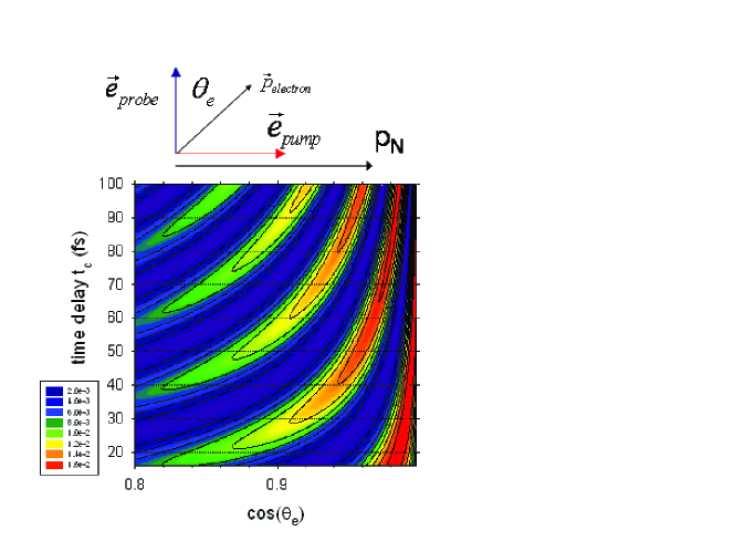
Figure 4: Same as in Fig.3. but for the case when the polarizations of the pump and probe pulses are perpendicular and the nuclear relative momentum $\vec{p}_{N}$ is also parallel to the polarization of the as shown in the upper part of the figure.

Assuming that initially ${\rm H_{2}^{+}}$ was at rest with the initial momentum of ${\rm H_{2}^{+}}$ centre of mass $\vec{P}_{CM}$ is zero, we have the following relations between the measured final momenta of the two protons $\vec{p}_{1}$, $\vec{p}_{2}$ and of the electron momentum $\vec{p}_{e}$ and the relative nuclear momentum $\vec{p}_{N}$:

$$\vec{p}_{1}+\vec{p}_{2}+\vec{p}_{e}=\vec{P}_{CM}=0\;\;\;\vec{p}_{N}=\frac{1}{2}(\vec{p}_{1}-\vec{p}_{2})$$ (33)

Consequently, if the initial molecular temperature is zero it will be sufficient to measure the electron momentum and the momentum of one proton $\vec{p}_{1}$ in order to determine the $\vec{p}_{N}$ vector on which the interference relies. Thus the vectors present in (21) formulas become:

$$\vec{p}_{N}=\vec{p}_{1}+\vec{p}_{e}/2\;\;,\;\;\vec{p}_{+}=\vec{p}_{1}+\vec{p}_{e}\;,\;\vec{p}_{-}=\vec{p}_{1}\;.$$ (34)

In the case of nonzero temperature of initial ${\rm H_{2}^{+}}$ translational motion one should either average our formula over thermal momenta of ${\rm H_{2}^{+}}$ or measure in coincidence the momenta of all three fragments resulting from the photoionization of dissociating ${\rm H_{2}^{+}}$ in order to avoid possible washing out of the interference term.

Summarizing, our most important result is that the Fano two-centre interference shows up in the cross term $C({p}_{+},{p}_{-},t_{c})$ in eq.(23) via

$$\cos\left(\vec{p}_{e}\cdot\vec{R}_{N}(t_{c},\vec{p}_{N})\right)\;$$ (35)

where $\vec{R}_{N}(t_{c},\vec{p}_{N})$ is given in eq.(28). Note, that the calculations in which $\vec{R}$ is fixed lead instead to the very similar interference term $\cos(\vec{p}_{e}\cdot\vec{R})$ in eq.(8). Thus the effect of nuclear motion consists in replacing $\vec{R}$ by $\vec{R}_{N}(t_{c},\vec{p}_{N})$ which is a simple linear function of the final relative momentum of outgoing protons $\vec{p}_{N}$ and of the time delay $t_{c}$. A convenient way to analyze this interference in the case of $\vec{p}_{N}$ fixed and parallel to the probe polarization $\vec{e}_{probe}$ (note then $\theta_{e}=\theta_{pe}$ which simplifies significantly eq.(32) is to expand the angular distributions described by (32) in Legendre polynomials $P_{l}(\cos\theta_{e})$:

$$|A_{fi}|^{2}\sim\cos^{2}\theta_{e}[1-\cos(p_{e}R\cos\theta_{e})]=\cos^{2}\theta_{e}\left[1-\sum_{l=0,l-even}^{\infty}(2l+1)j_{l}\left(p_{e}R(t_{c})\right)P_{l}(\cos\theta_{e})i^{l}\right]$$ (36)

$$|A_{fi}|^{2}\sim\beta_{0}(t_{c})+\beta_{2}(t_{c})P_{2}(\cos\theta_{e})+\beta_{4}(t_{c})P_{4}(\cos\theta_{e}),\mbox{ where}$$ (37)

$$\beta_{0}=\frac{1}{3}\left[1-j_{0}+2j_{2}\right]\simeq\frac{1}{3}\left[1-3\frac{\sin(p_{e}R_{N}(t_{c},p_{N}))}{p_{e}R_{N}(t_{c},p_{N})}\right]\mbox{ for }p_{e}R(t_{c})\gg 1$$ (38)

$$\beta_{2}=\frac{1}{3}\left[2-j_{0}+\frac{55}{7}j_{2}-\frac{36}{7}j_{4}\right]\simeq\frac{1}{3}\left[2-\frac{92}{7}\frac{\sin(p_{e}R_{N}(t_{c},p_{N}))}{p_{e}R_{N}(t_{c},p_{N})}\right]\mbox{ for }p_{e}R(t_{c})\gg 1$$ (39)

$$\beta_{4}=\frac{30}{11}j_{6}-\frac{351}{77}j_{4}\simeq\frac{51}{7}\frac{\sin(p_{e}R_{N}(t_{c},p_{N}))}{p_{e}R_{N}(t_{c},p_{N})}\mbox{ for }p_{e}R(t_{c})\gg 1\;\;.$$ (40)

We see clearly that the expansion of angular distributions in Legendre polynomials reveals the Fano interference as function of the pump-probe time delay $t_{c}$ in a very neat way. An analysis of experimental data related to the Fano interference using such an expansion was recently performed e.g. in Mabbs2005 . More specifically, in Mabbs2005 a pump-probe experiment was reported in which a pump pulse photodissociates a $I_{2}^{-}$ molecule and the probe photoionizes the dissociating molecule. The $\beta_{2}(t_{delay})$ coefficient calculated from the experimental photoelectron angular distribution shows the modulation similar to oscillations expected from our eq.(39). These experimental oscillations in $\beta_{2}(t_{delay})$ do not survive for the time delays larger than few picoseconds. We suggest that this maybe related to the constant term present in eq.(39) which shows in the experiment as background or they disappear due to averaging over nuclear momenta which becomes more significant at larger internuclear separations. Note, that the higher $\beta_{4}(t_{c})$ coefficient does not contain any constant term and thus may yield a better contrast allowing the Fano interference to survive for larger time delays.

III Some specific examples of the proposed pump-probe experiments

The interference expected from the theory presented in the previous section will show up most clearly when the proton and the electron momenta are measured in coincidence. Using our exact expressions (21) for probabilities as function of the momenta of three outgoing fragments we calculate the probabilities of ionization by the probe pulse for three selected geometries and plot the results in Figs.3-6. Note that we do not use in Figs.3-5 the approximations suggested in formulas (26),(30). The probabilities are shown as functions of the time delay $t_{c}$ between the pump and the probe pulse. We plot in Fig.3 the angular distributions of the electron in the parallel case, i.e. all three vectors $\vec{e}_{pump}$, $\vec{e}_{probe}$, and $\vec{p}_{N}$ are parallel and the momenta $p_{e}$ and $p_{N}$ are fixed at their maximal values. In Fig.4 the perpendicular geometry is used, i.e. we choose the case of the pump laser polarization $\vec{e}_{pump}$ perpendicular to polarization of the probe pulse $\vec{e}_{probe}$. In Fig. 6 again the geometry is parallel as in Fig.5 but instead of angular distributions we plot there the electron spectra for the electron flying along the polarization vectors. All three graphs show strong interference structures as function of the time delay, as expected from the approximate factor $\sin^{2}\left(\vec{p}_{e}\cdot\frac{\vec{p}_{N}}{|\vec{p}_{N}|}R_{N}(t_{c},p_{N})/2\right)\;.$ Note that we show in Fig.3 and in Fig.5 the positions of the centre of wave packet corresponding to certain time delays calculated using eq.(29). Similar interference structures appear in the proton spectra displayed in Fig.6 in which we are showing spectra as function of the single proton momentum $p_{1}=|\vec{p}_{1}|$ with fixed electron momentum $p_{e}$=0.72 a.u.. The $\vec{p}_{N}$ vector is calculated using eq.(34).

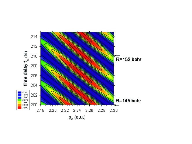
Figure 5: Same as in Fig.3. but for the shorter pump wavelength $\lambda_{probe}$=15 nm, shorter pulse duration $\tau_{FWHM}$=0.24 fs and smaller width of the wave packet $\Delta R$=1.0 bohr. Note that now the electron angle $\theta_{e}$ is fixed and equal to zero. The ionization probability is plotted now as function of the electron momentum $p_{e}$.

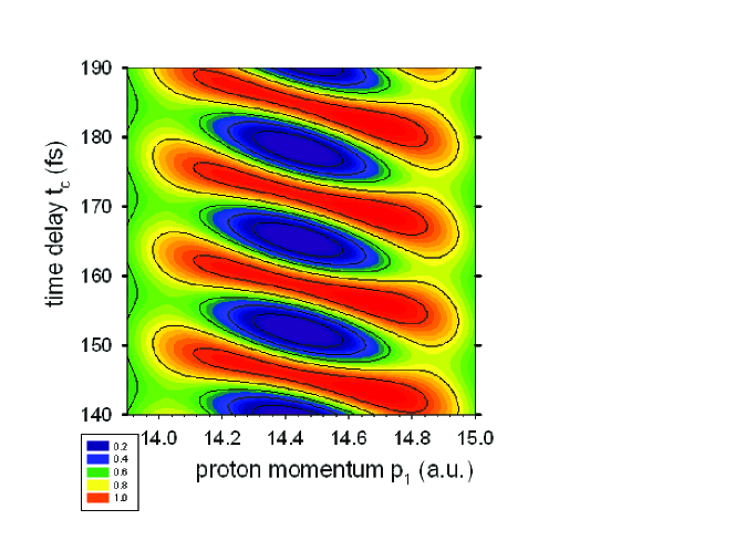
Figure 6: Same as in Fig.3. but now the ionization probability is plotted now as function of the proton momentum $p_{1}$ at fixed electron angle $\theta_{e}=0$

IV Concluding remarks

Summarizing, we have investigated a laser pump-probe scheme in which the measurement of the momenta distributions of the photelectron allow to determine the nuclear trajectory R(t) which simply plays a role of a slit separation in this double-slit like experiment in which the molecule is ”illuminated from within” Vrakking2009 . Thus the probe pulse prepares the electron source whose de Broglie wave create interference structure. The observed modulation as function of time delay, due to the change of the slit-separation becomes a witness of the simultaneous presence of the electron on each proton. In other words, when the internuclear distance R is much larger that the bohr orbit it would be natural to expect a localized electron on one heavy proton but such a localization would prevent the interference seen in the photoionization signal.

Another unusual feature of the proposed experimental scheme in this paper is the fact that it allows to measure, in a sense, the sign of the spatial wave function, more specificallly the measurment we propose detects (in the case of an ungerade initial state) the fact that the sign of electronic wave function on one centre is minus an an another remote centre is plus. Namely, at large internuclear distance the electronic wave function is given by :

$$\varphi_{el}^{g/u}=\frac{1}{\sqrt{2}}\left[\psi_{H}(\vec{r}_{e}+\vec{R}/2)\pm\psi_{H}(\vec{r}_{e}-\vec{R}/2)\right]\;\;.$$

Thus the probability density distribution $|\varphi_{el}^{g/u}(z)|^{2}$ is identical for both parities at very large R-values, see Fig.2. Nevertheless, measuring the photoelectron signal allows to distinguish between the gerade and ungerade case since the photoionization probability at fixed internuclear distance R is proportional to $\cos^{2}(\vec{p}_{e}\cdot\vec{R}/2)$ in the case of dissociation occurring on the gerade electronic state whereas is proportional to $\sin^{2}(\vec{p}_{e}\cdot\vec{R}/2)$ in the ungerade case. This sensitivity of the photoelectron spectra to parity (gerade or ungerade) is very specific to this simple dissociation process and because of this feature this experimental scheme is very distinct form the electron two-slit diffraction.

There exists already some experimental evidence for the existence of the Fano interferences originating from dissociating molecules at large internuclear separations: in the pump-probe experiment by Sanov et al Mabbs2005 negative iodine $I_{2}^{-}$ ions were used in which similar to dissociating ${\rm H_{2}^{+}}$ electron delocalization occur when a following pump-probe is used. The photoionization was initialized using a 780-nm laser that dissociated the $I_{2}^{-}$ ions into $I^{-}$ + neutral iodine atom I. After a variable time delay, a photoionizing probe removed the electron from the $I_{2}^{-}$ ion. Next the $\beta_{2}(t_{delay})$ coefficient, defined in our eqs.(37),(39) was calculated from the phototelectron angular distributions. This coefficient oscillates as function of the time delay between the probe and pump pulses as expected from eq.(39). This oscillation is due to the fact that as in our scheme one cannot distinguish whether the phototelectron originates from the right or left iodine atom separated by an internuclear distance as large as 60 bohr.

Another method for the observation of the two-centre interference was proposed in Bykov2003 . This method uses the probe pulse which does not ionizes the dissociating molecule but is based on elastic (Thomson) photon scattering from the two centres in the dissociating ${\rm H_{2}^{+}}$ . Thus this method, which resembles the double-slit experiment for photons, allows to probe the entangled state in dissociating ${\rm H_{2}^{+}}$ on the internuclear distance larger than the method discussed in our paper since the wavelength 800 nm laser is much larger than de Broglie wavelength used in our scheme. This method, as ours, shows the delocalization of the electron on two remote centres since both the Thomson scattering or phoionization (in the case of our method) rely on the presence of the electron on each centre, i.e neither Thomson scattering nor photonization can occur simply on bare proton. This fact distinguishes both schemes (ours and that proposed in Bykov2003 ) from a simple double-slit quantum effect.

Appendix A Beyond the Born-Oppenheimer approximation in the initial state

The Jacobi coordinates $\vec{r}_{e},\;\vec{R}$ used in the section II are not convenient at large internuclear distances R since the wave functions $\exp(i\vec{p}\cdot\vec{R})\varphi_{H}^{u}(\vec{r}_{e}\pm\vec{R})$ used in eq.(11) are not the exact eigenstates of the molecular Hamiltonian even if one neglects the Coulomb repulsion and the attraction from the remote bare proton. These states are approximate eigenstates, within the Born-Oppenheimer approximation. Note, that when a proton and an hydrogen atom are very far apart the exact eigenstates of $H_{0}$ are simply a product of two plane waves for: a free proton motion, free motion of the centre of mass of a hydrogen atom multiplied by the electronic wave function describing the 1s electronic state of the hydrogen atom. Thus when the proton and the hydrogen atom are far apart and they move with relative momentum $\vec{p}$ it is convenient to rewrite the Hamiltonian $H_{0}$ using different Jacobi coordinates from that used in section II. Namely, instead of using the internuclear vector $\vec{R}$ and the electron coordinate $\vec{r}_{e}$ we now use the vectors

$$\vec{R}_{1}=\vec{R}+\alpha\vec{r}_{1e}\;\;\mbox{where}\;\;\vec{r}_{1e}=\vec{r}_{e}-\vec{R}/2\;\;\mbox{and}\;\;\alpha={m_{e}\over m_{e}+m_{p}}.$$ (41)

$\vec{R}_{1}$ is the relative vector between the centre of mass of a hydrogen atom and the neighboring proton, $\vec{r}_{1e}$ is the relative vector between the proton and the electron. In these coordinates the Hamiltonian of ${\rm H_{2}^{+}}$ has the following form : (in atomic units, $\hbar=m_{e}=e$=1)

$$\hat{H}_{0}=-{1\over 2m^{\prime\prime}_{e}}\Delta_{\vec{r}_{1e}}-{1\over 2\mu^{\prime\prime}}\Delta_{\vec{R}_{1}}-{1\over|\vec{r}_{1e}|}+V_{2}(\vec{r}_{e},\vec{R})\;\;\mbox{where}\;V_{2}=-{1\over|\vec{r}_{e}+\vec{R}/2|}+{1\over R},$$ (42)

where

$$\mu^{\prime\prime}={m_{p}(m_{p}+m_{e})\over 2m_{p}+m_{e}}\;,\;m^{\prime\prime}_{e}=\;{m_{p}m_{e}\over m_{p}+m_{e}}\;,$$ (43)

and $m"e$ is simply the reduced mass of the electron in the hydrogen atom. Note that as in Jacobi coordinates used in section II there is no cross gradient term with coupling nuclear and electronic variables. We easily find the exact eigenstates of a dissociating wave packet with the relative momentum $\vec{p}$, in these new Jacobi coordinates, in the limit of very large internuclear distance when the potential $V_{2}(\vec{r}_{e},\vec{R})$ can be neglected. This exact asymptotic eigenstate has the following form:

$$\psi_{in}^{asym}(\vec{r}_{e},\vec{R},\vec{p})=\exp(i\vec{p}\cdot\vec{R}_{1})\psi_{H}(\vec{r}_{1e}))=\exp(i\vec{p}\cdot\left(\vec{R}+\alpha\vec{r}_{1e})\right)\psi_{H}(\vec{r}_{e}-\vec{R}/2)\;\;,$$ (44)

where $\vec{p}$ is the momentum of the relative motion between the hydrogen atom and the remote proton. Note that in contrast to the previously used eigenstate (11) the above state does not have the inversion symmetry with respect to the inversion $\vec{r}_{e}\rightarrow-\vec{r}_{e}$. Since we expect that the initial state should have such an inversion symmetry (as being prepared via one photon excitation of the gerade electronic state of a ${\rm H_{2}^{+}}$ molecule), we construct the ungerade initial state in the following way

$$\psi_{in}={1\over\sqrt{2}}\int d^{3}p\varphi_{N}(\vec{p},R_{0})\left[\psi_{in}^{asym}(-\vec{r}_{e},\vec{R},\vec{p})-\psi_{in}^{asym}(\vec{r}_{e},\vec{R},\vec{p})\right]\;\;.$$ (45)

Clearly, for each fixed $\vec{p}$ this is an entangled state of the two particles: a free proton and a free hydrogen atom. We rewrite the interaction potential (4) in a slightly different form :

$$\hat{V}_{int}=-i\vec{A}(t)\cdot\left({1\over m_{e}}\nabla_{\vec{r}_{e}}-i{1\over m_{p}}\nabla_{\vec{r}_{1p}}-i{1\over m_{p}}\nabla_{\vec{r}_{2p}}\right)=-i{1\over m^{\prime\prime}_{e}c}\vec{A}(t)\cdot\nabla_{\vec{r}_{1e}}-i{1\over m_{p}}\vec{A}(t)\cdot\nabla_{\vec{r}_{2p}}\;\;$$ (46)

Note that we keep here the complete interaction of the laser field $\vec{A}(t)$ with three charges whereas in the previous Jacobi coordinates (4) the interaction term with coupling to the system centre of mass was not included. In the last term in the above formula we have merged together the interaction of the electron with the proton which binds the electron. The last term in eq.(46 will be neglected in the matrix element (5) since it describes the interaction of the bare proton in the case when we evaluating the term containing $\psi_{H}(\vec{r}_{1e})$, and vice versa for the term with $\psi_{H}(\vec{r}_{2e})$. Inserting this new initial state (45) into the eq.(5) we get

$$\tilde{A}_{fi}=\tilde{N}_{2}\left[A_{H}(\vec{p}_{e}+\alpha\vec{p}_{-})\tilde{a}(\vec{p}_{-})-A_{H}(\vec{p}_{e}-\alpha\vec{p}_{+})\tilde{a}(\vec{p}_{+})\right]$$ (47)

where

$$\tilde{a}(\vec{p})=\exp[i\tilde{f}(\vec{p})t_{c}-\tau^{2}\tilde{f}(\vec{p})/2]\varphi_{N}(\vec{p},R_{0})\;\;,$$ (48)

and

$$\tilde{f}(\vec{p})={\vec{p}\;^{2}_{e}\over 2m^{\prime}_{e}}+{\vec{p}\;^{2}_{N}\over 2\mu}+I_{p}-\Omega_{probe}-{\vec{p}\;^{2}\over 2\mu^{\prime\prime}}\;\;,\tilde{N}_{2}=(2\pi)^{2}{A_{0}\tau\over 2^{3/2}m^{\prime\prime}_{e}c}\;,\;$$ (49)

We note that using exact non-Born-Oppenheimer asymptotic (for large R) states leads to the two following modifications in the transition amplitude as compared with (18). First, the atomic transition amplitude does not factorize, second, the function $f(\vec{p})$ contains different reduced mass $\mu"$. The first modification has a simple interpretation: since the nuclei move in the opposite direction the relative electron momentum is different on each centre (proton). Since the atomic amplitude $A_{H}$ is now different at each centre previous eqs.(21)-(23) will be modified in the following way:

$$|\tilde{A}_{fi}(\vec{p}_{e},\vec{p}_{N},\tau,\Delta R,t_{c})|^{2}=|A_{H}(\vec{p}_{e}+\alpha\vec{p}_{-})|^{2}|\tilde{a}(\vec{p}_{-}|^{2}+|A_{H}(\vec{p}_{e}-\alpha\vec{p}_{+})|^{2}|\tilde{a}(\vec{p}_{-}|^{2}+\tilde{C}({p}_{+},{p}_{-},t_{c})$$ (50)

where

$$\tilde{C}({p}_{+},{p}_{-},t_{c})=2|a(\vec{p}_{+})|\;|a(\vec{p}_{-})||A_{H}(\vec{p}_{e}+\alpha\vec{p}_{-})||A_{H}(\vec{p}_{e}-\alpha\vec{p}_{+})|\cos(\tilde{\Phi}(t_{c},))\;\;,$$ (51)

$$\tilde{\Phi}(t_{c},\vec{p}_{e},\vec{p}_{N})=(|\vec{p}_{+}|-|\vec{p}_{-}|)\;R_{0}+\varphi_{H}(\vec{p}_{e}+\alpha\vec{p}_{-})-\varphi_{H}(\vec{p}_{e}-\alpha\vec{p}_{+})\;+\;\vec{p}_{e}\cdot{\vec{p}_{N}\over\mu^{\prime\prime}}\;t_{c}\;\;$$ (52)

where the phase $\varphi_{H}(\vec{p})$ is simply the phase of the atomic amplitude $A_{H}$ defined in eq.(16), i.e.

$$A_{H}(\vec{p})=|A_{H}(\vec{p})|\exp[i\varphi_{H}(\vec{p})]\;\;.$$ (53)

We conclude that the Fano interference will be similar when the non-Born-Oppenheimer correction is included. The only change in the time delay dependent part is a replacement of the reduced mass $\mu$ by the mass $\mu^{\prime\prime}$. Another change, due to shift of the argument in the $A_{H}(\vec{p})$ function modifies only the term which does not depend on the time delay $t_{c}$. Moreover the modifications discussed in this section will be negligible for the cases studied in section III where the values of the electron and nuclear momenta are $p_{e}=0.72$, $p_{N}=$14.8 a.u., respectively, and $\alpha=1/1836$ is indeed small. Thus we do not expect that the shifts in a slowly varying function $A_{H}(\vec{p})$ will modify significantly the predictions relative to our ”dynamic” Fano interference factor (23) and illustrated in previous sections in Figs.3-6.

- (1) A. Einstein, B. Podolsky, and N. Rosen, Phys.Rev. 47, 777 (1935).
- (2) M.D. Reid, P.D. Drummond, W.P. Bowen, E.G. Cavalcanti, P.K. Lam, H.A. Bachor, U.L. Andresen, and G. Leuchs, J. Mod. Phys. 81, 1727 (2009).
- (3) A. Ekert, Phys. World 22, Issue 9, 29 (2009).
- (4) M. Aspelmeyer and A. Zeilinger, Phys. World 21, Issue 7, 22 (2008).
- (5) J. Dunningham and V. Vedral, Phys.Rev.Lett. 99, 180404 (2007).
- (6) M.V. Fedorov, M.A. Efremov, P.A. Volkov, and J.H. Eberly, J. Phys. B 39, S467 (2006).
- (7) M.V. Fedorov, M.A. Efremov, A.E Kazakov, K.W. Chan, C.K. Law, and J.H. Eberly, Phys. Rev. A 69 , 052117 (2004).
- (8) E.S. Fry, T. Walther, and S. Li, Phys.Rev. A 52 4381 (1995).
- (9) C. Gneiting and K. Hornberger, Phys.Rev.Lett. 101, 260503 (2008).
- (10) T. Opartny and G. Kurizki, Phys.Rev. Lett. 86, 3180 (2001).
- (11) C.N. Savage and K.V. Kheruntsyan, Phys.Rev.Lett. 99, 220404 (2007).
- (12) F. Krausz and M. Ivanov, Rev. Mod. Phys. 81, 163 (2009).
- (13) M. Vrakking, Physics, 2, 72 (2009). http://link.aps.org/doi/10.1103/Physics.2.72
- (14) H.D. Cohen and U. Fano 150, 30 (1966).
- (15) V.P. Bykov and E. Nahvifard, Las.Phys. 13, 501 (2003).
- (16) J.J. Sakurai, Modern Quantum Mechanics, Section 3.9 (The Benjamin/Cummings publishing Company, Menlo Park (1985)).
- (17) G.L. Yudin, S. Chelkowski, and A.D. Bandrauk, J. Phys. B 39, L17 (2006).
- (18) V.P. Bykov, Physics-Uspekhi 49(9), 979 (2006).
- (19) A.D. Bandrauk, S. Chelkowski, P.B. Corkum, J. Manz, and G.L. Yudin, J. Phys. B 42, 134001 (2009).
- (20) A.D. Bandrauk and S. Chelkowski, Phys.Rev.Lett. 87, 273004 (1999).
- (21) J.R. Hiskes, Phys.Rev. 122, 1207 (1961).
- (22) R. Mabbs, K. Pichugin, and A. Sanov, J. Chem. Phys. 123, 054329 (2005); R. Mabbs, K. Pichugin, and A. Sanov, J.Chem.Phys. 122, 174305 (2005).