Anderson Model out of equilibrium: decoherence effects in transport through a quantum dot

Abstract

The paper deals with the nonequilibrium two-lead Anderson model, considered as an adequate description for transport through a d-c biased quantum dot. Using a self-consistent equation-of-motion method generalized out of equilibrium, we calculate a fourth-order decoherence rate $\gamma^{(4)}$ induced by a bias voltage $V$. This decoherence rate provides a cut-off to the infrared divergences of the self-energy showing up in the Kondo regime. At low temperature, the Kondo peak in the density of states is split into two peaks pinned at the chemical potential of the two leads. The height of these peaks is controlled by $\gamma^{(4)}$. The voltage dependence of the differential conductance exhibits a zero-bias peak followed by a broad Coulomb peak at large $V$, reflecting charge fluctuations inside the dot. The low-bias differential conductance is found to be a universal function of the normalized bias voltage $V/T_{K}$, where $T_{K}$ is the Kondo temperature. The universal scaling with a single energy scale $T_{K}$ at low bias voltages is also observed for the renormalized decoherence rate $\gamma^{(4)}/T_{K}$. We discuss the effect of $\gamma^{(4)}$ on the crossover from strong to weak coupling regime when either the temperature or the bias voltage is increased.

I Introduction

Over the last ten years, an intense experimental and theoretical activity has been developed to study quantum dots. Due to the presence of strong electronic correlations in the dot, these mesoscopic systems give rise to rich collective phenomena such as the Coulomb blockade and the Kondo effect. Their manifestations in transport can be studied in a detailed and controlled way in such devices as semiconductor-based quantum dots embedded in a two-dimensional electron gasGoldhaber1998 or carbon nanotubesNygard00 . One of the great interests of these systems is to offer the possibility of studying them under nonequilibrium conditions when either a bias voltage is applied to the leads or an electromagnetic field irradiates the device.

A simple model describing quantum dots is the Anderson modelAnderson61 , in which the dot is represented by a localized level connected to Fermi seas of conduction electrons through tunneling barriers. When the dot is singly occupied, it has been shown that the linear conductance increases as one lowers the temperature, and eventually reaches the unitary limit $2e^{2}/h$ in the case of symmetric coupling to the leads. This was predicted in the context of quantum dots twenty years agoGlazman88 ; Ng88 and was observed experimentally about ten years laterGoldhaber1998 ; Nygard00 .

While in equilibrium most of the properties of the Kondo effect are now well understoodHewson thanks to the development of a panel of powerful techniques (e.g. renormalization group, Bethe ansatz, Fermi-liquid theory, conformal field theory, density matrix renormalization group, slave boson and equation-of-motion approaches), most of these techniques fail out of equilibrium. Hence there is a huge interest to develop new techniques to tackle the problem of the Kondo effect out of equilibrium and more generally nonequilibrium effects in strongly-correlated electron systems.

Theoretically, the Kondo effect out of equilibrium has been investigated by a variety of techniques developed most of the time within the Keldysh formalism: perturbation theory and perturbative renormalization group approachKaminski00 ; Coleman2001 ; Parcollet02 ; Rosch2001 ; Rosch2003 ; Rosch2004 , slave-boson formulation solved by using either mean-fieldAguado00 or non-crossing approximationWingreenPRB94 , equation-of-motion approachesMonreal2005 ; Swirkowicz03 . Exact solutions at the Toulouse limit have been proposedSchiller95 . Other ones have extended the Bethe ansatz out of equilibriumKonik01 ; Konik02 , and in some cases have used the results to construct a Landauer-type picture of transport through the quantum dot. There have also been important efforts to develop numerical techniques such as time-dependent Numerical Renormalisation GroupBulla08 ; Anders2008 and imaginary-time theory solved by using Quantum Monte CarloHanHeary2007 . All those approaches have only a limited validity of their parameter regimes since they mostly describe the properties of the system in its ground state, and not in its excited many-body states reached when the bias voltage drives a current through the dot.

In this paper, we develop an equation-of-motion (EOM) approach to tackle the nonequilibrium Kondo effect in quantum dots and study the decoherence effects induced by a bias voltage. The EOM method, though conceptually simple, requires some care. The recursive application of the Heisenberg equation of motionZubarev60 generates an infinite hierarchy of equations, which relate the different Green functions of the system. This hierarchy has to be truncated by a suitable approximation scheme in order to form a closed set of equations. The choice of the truncation scheme is crucial in order to treat carefully the correlation effects both from the Coulomb interaction and from the dot-lead tunneling.

The EOM technique was applied to the original Anderson model at equilibrium a long time agoDworin1967 ; Appelbaum1969 ; Theumann69etal ; Lacroix1981 in the context of the dilute magnetic alloys. When applying the standard approximation based on a truncation of the equations of motion at second order in the hybridization term $t_{\sigma}$, it yields results which agree with perturbation theory calculations for temperatures above the Kondo temperature, $T_{K}$. This truncation scheme is usually referred to as the Lacroix approximationLacroix1981 . Even though the scheme has serious drawbacks at this level of approximation (underestimation of the Kondo temperature $T_{K}$, absence of Kondo effect just at the particle-hole symmetric point), it is acknowledged to provide a valuable basis for the description of the Kondo effect both at high and low temperatures. The applicability of the Lacroix approximation is nicely reported in a recent paper by V. Kashcheyevs et alKashcheyevs2006 .

In the early nineties, Meir, Wingreen, and LeeMWL1993 undertook to apply the EOM method to the study of quantum dots out of equilibrium and/or in the presence of a magnetic field. They used a simplified version of the Lacroix approximation, which fails to account for the finite decoherence rates induced by bias voltage and/or magnetic field. Meir et al. proposed to introduce them heuristically by making use of the Fermi golden rule. They obtained interesting results for the bias voltage dependence of the differential conductance showing a zero-bias anomaly, but the weakness of the approach is that it does not constitute an unified and consistent frame for the treatment of the Kondo effect in the presence of the decoherence effects induced out of equilibrium.

There have been recent attempts to use an approximation which truncates the equations of motion at higher order in $t_{\sigma}$ Monreal2005 ; Luo1999 ; Swirkowicz03 . Their authors claimed to improve quantitatively at equilibrium the Kondo temperature and the density of states around the Fermi energy and have been able to investigate some nonequilibrium issues. However, there is need to clarify the decoherence effects in the framework of the EOM method.

The organization of the paper is the following:

- In Sec.II, we outline the EOM formalism and the main steps of the proposed approximation based on a truncation of the equations of motion at the fourth order in $t_{\sigma}$. An analytical expression of the retarded Green function in the dot is derived involving expectation values which are determined self-consistently. The details of the calculations are presented in Appendix I and Appendix II.

- An analytical study of this Green function is presented in Sec.III. Namely, we deduce the renormalization effects and the transition rates involved at the second order in $t_{\sigma}$ for the different regimes of the Anderson model. Special care is given to the singly-occupied dot regime, for which the vanishing of one of the transition rates leads to the low-energy logarithmic divergence of the self-energy of the dot Green function, yielding a Kondo resonance peak in the density of states. We show how the approximation scheme allows one to derive a decoherence rate out of equilibrium which becomes finite as soon as a bias voltage is applied. This decoherence rate provides a cut-off to the logarithmic divergence present at equilibrium in the Kondo regime. We show how our approximation scheme improves the result for the Kondo temperature $T_{K}$ upon earlier predictions.

- We present in Sec.IV our numerical results - both at equilibrium and out of equilibrium - for the density of states, the (linear and differential) conductance and the bias-induced decoherence rate. A self-consistent treatment is required in order to determine the expectation values involved in the Green function of the dot. At equilibrium, the density of states in the particle-hole symmetric case shows a three-peak structure at low temperature with a Kondo resonance peak in the local moment regime. This result constitutes an advantage of our approximation scheme compared to the Lacroix approximation. The unitary limit for the linear conductance $G=2e^{2}/h$ is analytically recovered at zero temperature in the particle-hole symmetric case when the dot is symmetrically coupled to the leads. Numerically, one notices a slight underestimation of $G$ due to the numerical accuracy of the self-consistent treatment.

Out of equilibrium, the spectral function shows a splitting of the Kondo peak into two peaks pinned at the chemical potentials of the two leads. The height of the peaks diminishes when the bias voltage increases, meaning that the Kondo effect is destroyed by decoherence induced out of equilibrium. This influences the evolution of the differential conductance as a function of bias voltage, which shows a zero-bias anomaly followed by a broad Coulomb peak. At low bias voltage, we check that the differential conductance follows a universal scaling law which depends on a single energy scale, $T_{K}$. Comparison is made with results obtained by recent numerical techniques for nonequilibrium such as time-dependent NRGAnders2008 and imaginary time theory solved by QMCHanHeary2007 ; Han2009 .

Finally, we compute the bias voltage dependence of the decoherence rate and discuss the crossover from strong coupling to weak coupling regime depending on the comparison between the decoherence rate and a characteristic energy scale $T^{*}$. We show the existence of a crossover between the strong coupling and weak coupling regime when either the temperature or the bias voltage is raised, as predicted by other methods.

II Equation-of-motion formalism

We model the quantum dot connected to the two leads by the single-level (spin-1/2) Anderson impurity hamiltonian

$$\mathcal{H} = H_{lead}+H_{dot}+H_{int},$$ (1)

$$H_{lead} = \displaystyle\sum_{\alpha k\sigma}\varepsilon_{\alpha k}c_{\alpha k\sigma}^{{\dagger}}c_{\alpha k\sigma},$$

$$H_{dot} = \sum_{\sigma}\varepsilon_{\sigma}n_{\sigma}+Un_{\uparrow}n_{\downarrow},$$

$$H_{int} = \displaystyle\sum_{\alpha k\sigma}(t_{\alpha\sigma}c^{{\dagger}}_{\alpha k\sigma}f_{\sigma}+H.C.),$$

where $c_{\alpha k\sigma}^{{\dagger}}(c_{\alpha k\sigma})$ is the creation (annihilation) operator of an electron of momentum $k$ and spin $\sigma(=\pm 1)$ in the $\alpha(=L,~{}R)$ lead (with energy $\varepsilon_{\alpha k}=\varepsilon_{k}-\mu_{\alpha})$; $\mu_{\alpha}$ is the chemical potential in the $\alpha$ lead; $f_{\sigma}^{{\dagger}}(f_{\sigma})$ is the creation (annihilation) operator of an electron of spin $\sigma$ in the quantum dot (with energy $\varepsilon_{\sigma}=\varepsilon_{d}+\sigma B/2$ when the Zeeman splitting $B$ is included); $n_{\sigma}=f_{\sigma}^{\dagger}f_{\sigma}$ is the number operator for electrons of spin $\sigma$ in the dot; $U$ is the Coulomb interaction between two electrons of opposite spin in the dot; and $t_{\alpha\sigma}$ is the tunneling matrix element between the state $|k\sigma\rangle$ in the $\alpha$ lead, and the state $|\sigma\rangle$ in the dot. For simplicity, we assume $t_{\alpha\sigma}$ to be real and $k$-independent.

When a bias voltage is applied to the leads $(eV=\mu_{L}-\mu_{R})$, the system is driven out of equilibrium and a current is induced through the quantum dot. The current $I$ for the Anderson model is expressed by the generalized Landauer formulaMW92 accounting for the interactions among electrons

$$I=\frac{2e}{\hbar}\sum_{\sigma}\int_{-W}^{W}d\varepsilon\frac{\Gamma_{L\sigma}(\varepsilon)\Gamma_{R\sigma}(\varepsilon)}{\Gamma_{L\sigma}(\varepsilon)+\Gamma_{R\sigma}(\varepsilon)}[f_{F}^{L}(\varepsilon)-f_{F}^{R}(\varepsilon)]\rho_{\sigma}(\varepsilon),$$ (2)

where

• $W$ is the half-bandwidth of the conduction electron band in the leads,

• $\Gamma_{\alpha\sigma}(\varepsilon)$ is the tunneling rate of the spin $\sigma$ dot electron at energy $\varepsilon$ into the lead $\alpha$, defined as $\Gamma_{\alpha\sigma}(\varepsilon)=\pi\sum_{k}t_{\alpha\sigma}^{2}\delta(\varepsilon-\varepsilon_{\alpha k})=\pi t_{\alpha\sigma}^{2}\rho_{\alpha}^{0}(\varepsilon)$ with $\rho_{\alpha}^{0}(\varepsilon)$ the unrenormalized density of states at energy $\varepsilon$ in the lead $\alpha$,

• $f_{F}^{\alpha}(\varepsilon)=\{{\rm exp}\left[\beta(\varepsilon-\mu_{\alpha})\right]+1\}^{-1}$ is the Fermi-Dirac distribution function in the $\alpha$ lead,

• $\rho_{\sigma}(\varepsilon)$, the local density of states for spin $\sigma$ in the dot, can be expressed in terms of the retarded electron Green function in the dot $\mathcal{G}_{\sigma}^{r}(\varepsilon)$ according to $\rho_{\sigma}(\varepsilon)=-1/\pi{\rm Im}\mathcal{G}_{\sigma}^{r}(\varepsilon)$.

As pointed out in Ref.MW92, , Eq.(2) is valid provided that the tunneling couplings for both leads $\Gamma_{L\sigma}(\varepsilon)$ and $\Gamma_{R\sigma}(\varepsilon)$ differ only by a constant multiplicative factor.

The task is to compute the retarded electron Green function in the dot defined as $\mathcal{G}_{\sigma}^{r}(\omega)=-i\int_{0}^{\infty}dte^{i\zeta t}\langle\{f_{\sigma}(t),f_{\sigma}^{{\dagger}}(0)\}\rangle$ where $\zeta=\omega+i\delta$ ($\delta\rightarrow 0^{+}$). In order to simplify the notations in the rest of the paper, the imaginary part $i\delta$ going alongside $\omega$ will be implicit, while the summation over $k$ implies summation over both $\alpha$ and $k$. Hence we write in a shorthand notation

$$\sum_{\alpha=L,R}\sum_{k}t_{\alpha\sigma}\longrightarrow\sum_{k}t_{\sigma}.$$

Using the Zubarev notationZubarev60 for the retarded Green functions involving fermionic operators $A$ and $B$

$$\langle\langle A,B\rangle\rangle=-i\;\lim_{\delta\rightarrow 0^{+}}\;\int^{\infty}_{0}dt\;e^{i(\omega+i\delta)t}\;\langle\{A(t),B(0)\}\rangle,$$ (3)

which can be integrated by parts, and using the Heisenberg equation of motion, one can show the following relation

$$\omega\langle\langle A,B\rangle\rangle=\langle\{A,B\}\rangle+\langle\langle[A,H],B\rangle\rangle.$$ (4)

This allows us to derive a flow of equations for the dot Green function $\mathcal{G}^{r}_{\sigma}(\omega)\equiv\langle\langle f_{\sigma},f_{\sigma}^{{\dagger}}\rangle\rangle$. We also adopt a simpler notation in the following derivations by changing

$$\langle\langle A,f_{\sigma}^{{\dagger}}\rangle\rangle\longrightarrow\langle\langle A\rangle\rangle.$$

Applying Eq. (4), we find the first equations of motion

$$(\omega-\varepsilon_{\sigma})\langle\langle f_{\sigma}\rangle\rangle = 1+\sum_{k}t_{\sigma}\langle\langle c_{k\sigma}\rangle\rangle+U\langle\langle n_{\bar{\sigma}}f_{\sigma}\rangle\rangle,$$ (5)

$$(\omega-\varepsilon_{k})\langle\langle c_{k\sigma}\rangle\rangle = t_{\sigma}\langle\langle f_{\sigma}\rangle\rangle.$$ (6)

Combining Eqs. (5, 6) yields

$$[\omega-\varepsilon_{\sigma}-\Sigma^{0}_{\sigma}(\omega)]\langle\langle f_{\sigma}\rangle\rangle=1+U\langle\langle n_{\bar{\sigma}}f_{\sigma}\rangle\rangle,\\$$ (7)

where $\Sigma^{0}_{\sigma}(\omega)=\displaystyle\sum_{k}\frac{t_{\sigma}^{2}}{\omega-\varepsilon_{k}}$. Eqs. (5,6) are referred to as the first-generation equations of motion in the hierarchy. They govern the evolution of the Green functions formed by a single operator (i.e. $\langle\langle f_{\sigma}\rangle\rangle$ and $\langle\langle c_{k\sigma}\rangle\rangle$).

Throughout this paper, we assume that the half-bandwidth $W$ is much larger than all the other energy scales, so that the band edge effect does not affect the local density of states in the dot $\rho_{\sigma}(\omega)$. In this case, the properties of the system at low temperatures do not depend on the exact value of $W$ since only states around the Fermi level contribute, justifying the consideration of the wide-band limitAppelbaum1969 $W\rightarrow\infty$. Within this limit, the non-interacting self-energy can be approximated by $\Sigma^{0}_{\sigma}(\omega)\simeq-i\Gamma_{\sigma}$, where $\Gamma_{\sigma}(=\Gamma_{L\sigma}+\Gamma_{R\sigma})$ is a constant, independent of energy.

Interesting dynamics comes from $\langle\langle n_{\bar{\sigma}}f_{\sigma}\rangle\rangle$; its equation of motion is given by

$$[\omega-\varepsilon_{\sigma}-U]\langle\langle n_{\bar{\sigma}}f_{\sigma}\rangle\rangle=\langle n_{\bar{\sigma}}\rangle+\sum_{k}\Big{[}t_{\sigma}\langle\langle n_{\bar{\sigma}}c_{k\sigma}\rangle\rangle$$ (8)

$$+t_{\bar{\sigma}}\langle\langle f^{{\dagger}}_{\bar{\sigma}}c_{k{\bar{\sigma}}}f_{\sigma}\rangle\rangle-t_{\bar{\sigma}}\langle\langle c_{k{\bar{\sigma}}}^{{\dagger}}f_{\bar{\sigma}}f_{\sigma}\rangle\rangle\Big{]}.$$

The Green functions appearing on the right-hand side of Eq. (8) have their evolution governed by the following equations

$$\omega_{:k}\langle\langle n_{\bar{\sigma}}c_{k\sigma}\rangle\rangle&=t_{\sigma}\langle\langle n_{\bar{\sigma}}f_{\sigma}\rangle\rangle+\sum_{k^{\prime}}t_{\bar{\sigma}}\Big{[}\langle\langle f_{\bar{\sigma}}^{{\dagger}}c_{k^{\prime}{\bar{\sigma}}}c_{k\sigma}\rangle\rangle-\langle\langle c_{k^{\prime}{\bar{\sigma}}}^{{\dagger}}f_{\bar{\sigma}}c_{k\sigma}\rangle\rangle\Big{]},\\ \omega_{{\bar{\sigma}}:\sigma k}\langle\langle f_{\bar{\sigma}}^{{\dagger}}c_{k{\bar{\sigma}}}f_{\sigma}\rangle\rangle=\langle f_{\bar{\sigma}}^{{\dagger}}c_{k{\bar{\sigma}}}\rangle+t_{{\bar{\sigma}}}\langle\langle n_{\bar{\sigma}}f_{\sigma}\rangle\rangle+\sum_{k^{\prime}}\Big{[}t_{\sigma}\langle\langle f_{\bar{\sigma}}^{{\dagger}}c_{k{\bar{\sigma}}}c_{k^{\prime}\sigma}\rangle\rangle-t_{{\bar{\sigma}}}\langle\langle c_{k^{\prime}{\bar{\sigma}}}^{{\dagger}}c_{k{\bar{\sigma}}}f_{\sigma}\rangle\rangle\Big{]},\\ \left(\omega_{k:\sigma{\bar{\sigma}}}-U\right)\langle\langle c_{k{\bar{\sigma}}}^{{\dagger}}f_{\bar{\sigma}}f_{\sigma}\rangle\rangle=\langle c_{k{\bar{\sigma}}}^{{\dagger}}f_{\bar{\sigma}}\rangle-t_{\bar{\sigma}}\langle\langle n_{\bar{\sigma}}f_{\sigma}\rangle\rangle+\sum_{k^{\prime}}\Big{[}t_{\bar{\sigma}}\langle\langle c_{k{\bar{\sigma}}}^{{\dagger}}c_{k^{\prime}{\bar{\sigma}}}f_{\sigma}\rangle\rangle+t_{\sigma}\langle\langle c_{k{\bar{\sigma}}}^{{\dagger}}f_{\bar{\sigma}}c_{k^{\prime}\sigma}\rangle\rangle\Big{]}.$$ (9)

where we write in a shorthand notation

$$\omega_{\alpha\beta\cdots:ab\cdots} \equiv \omega+\varepsilon_{\alpha}+\varepsilon_{\beta}+\cdots-\varepsilon_{a}-\varepsilon_{b}-\cdots,$$

with $\{\alpha\beta\cdots,ab\cdots\}$ being any set of parameters within ${k}$’s and ${\sigma}$’s. We have for instance: $\omega_{:k}\equiv\omega-\varepsilon_{k}$, $\omega_{k:}\equiv\omega+\varepsilon_{k}$, $\omega_{{\bar{\sigma}}:k\sigma}\equiv\omega+\varepsilon_{\bar{\sigma}}-\varepsilon_{k}-\varepsilon_{\sigma}$, and $\omega_{k:\sigma{\bar{\sigma}}}\equiv\omega+\varepsilon_{k}-\varepsilon_{\sigma}-\varepsilon_{\bar{\sigma}}$.

Eqs. (9) generate three new Green functions on their right-hand side. Generally one can divide the expressions of the latter Green functions into two parts

$$\langle\langle f_{\bar{\sigma}}^{\dagger}c_{k{\bar{\sigma}}}c_{k^{\prime}\sigma}\rangle\rangle&=\langle f_{\bar{\sigma}}^{\dagger}c_{k{\bar{\sigma}}}\rangle\langle\langle c_{k^{\prime}\sigma}\rangle\rangle+\langle\langle f_{\bar{\sigma}}^{\dagger}c_{k{\bar{\sigma}}}c_{k^{\prime}\sigma}\rangle\rangle_{c},\;\;\\ \langle\langle c_{k{\bar{\sigma}}}^{\dagger}f_{\bar{\sigma}}c_{k^{\prime}\sigma}\rangle\rangle=\langle c_{k{\bar{\sigma}}}^{\dagger}f_{\bar{\sigma}}\rangle\langle\langle c_{k^{\prime}\sigma}\rangle\rangle+\langle\langle c_{k{\bar{\sigma}}}^{\dagger}f_{\bar{\sigma}}c_{k^{\prime}\sigma}\rangle\rangle_{c},\;\;\\ \langle\langle c_{k{\bar{\sigma}}}^{\dagger}c_{k^{\prime}{\bar{\sigma}}}f_{\sigma}\rangle\rangle=\langle c_{k{\bar{\sigma}}}^{\dagger}c_{k^{\prime}{\bar{\sigma}}}\rangle\langle\langle f_{\sigma}\rangle\rangle+\langle\langle c_{k{\bar{\sigma}}}^{\dagger}c_{k^{\prime}{\bar{\sigma}}}f_{\sigma}\rangle\rangle_{c}.\;\;$$ (10)

where the first part is obtained by decoupling pairs of same-spin operators and the second part $\langle\langle\cdots\rangle\rangle_{c}$ defines connected Green functions in the spirit of cumulant expansion. It is often assumed that these connected Green functions are negligible. This assumption has been broadly applied, usually referred to as the Lacroix approximationLacroix1981 . It turns out that within this approximation, the calculation of $\langle\langle f_{\sigma}\rangle\rangle$ is exact at the second order in $t_{\sigma}$, while it picks up some of the fourth-order contributions. At zero temperature, this approximation leads to logarithmic singularities in the density of states of the dot at the chemical potential, even in the presence of an external magnetic field $B$ or a bias voltage $V$. These divergences are unphysical since one expects the logarithmic singularities to be washed out by decoherence effects introduced by either $B$ or $V$.

In this work, we propose to go beyond the Lacroix approximation, and consider higher hierarchy in the equations of motion. The interest of the approach is to account for the decoherence effects introduced by either nonequilibrium or the presence of a magnetic field. The detailed derivation of the higher-hierarchy equations of motion and the decoupling scheme are given in Appendix I. In the approximation scheme we propose, after having expanded the equations of motion to order $t_{\sigma}^{4}$, we decouple pairs of same-spin lead electron operators (e.g. $\langle c_{{k^{\prime}}\sigma}^{\dagger}c_{k\sigma}\rangle$) and pairs of same-spin dot-lead electron operators (e.g. $\langle c_{k\sigma}^{\dagger}f_{\sigma}\rangle$ and $\langle f_{\sigma}^{\dagger}c_{k\sigma}\rangle$). This decoupling has to be done carefully in order to avoid double counting. The equations of motion of the three functions on the left-hand-side of Eqs. (8) are given by Eqs. (A.12), which are exact up to order $t_{\sigma}^{4}$.

Combining Eqs. (7, 8, A.12) yields a rather complex expression for $\langle\langle f_{\sigma}\rangle\rangle$ since Eqs. (A.12) couple to each other in an integral way. In this paper we will limit ourselves to a simple expression for the Green function $\langle\langle f_{\sigma}\rangle\rangle$ that neglects contributions generated through integral coupling of the equations of motion. This is motivated by the fact that the contributions we keep effectively lead to a second order term after resummation, as shown later on. The integral terms we neglect, on the contrary, are at least of fourth order in $t_{\sigma}$ and we believe they are not relevant for our study of the decoherence effects at nonzero bias and/or temperature. Thus, we are able to reduce Eqs. (A.12) to

$$\big{[}\omega_{:k}-\Sigma_{1\sigma}(\omega_{:k})\big{]}\langle\langle n_{\bar{\sigma}}c_{k\sigma}\rangle\rangle&=t_{\sigma}\langle\langle n_{\bar{\sigma}}f_{\sigma}\rangle\rangle+\Sigma_{5{\bar{\sigma}}}(\omega_{:k})\langle\langle n_{\sigma}c_{k\sigma}\rangle\rangle,\\ \big{[}\omega_{{\bar{\sigma}}:k\sigma}-\widehat{\Sigma}_{2\sigma}(\omega_{:k})\big{]}\langle\langle f_{\bar{\sigma}}^{{\dagger}}c_{k{\bar{\sigma}}}f_{\sigma}\rangle\rangle=\langle f_{\bar{\sigma}}^{{\dagger}}c_{k{\bar{\sigma}}}\rangle+t_{{\bar{\sigma}}}\langle\langle n_{\bar{\sigma}}f_{\sigma}\rangle\rangle-\sum_{k^{\prime}}\Big{[}t_{\bar{\sigma}}f_{{k^{\prime}}k}^{\bar{\sigma}}+\langle f_{\bar{\sigma}}^{\dagger}c_{k{\bar{\sigma}}}\rangle t^{2}_{\sigma}D_{{\bar{\sigma}}:k{k^{\prime}}}\sum_{{k^{\prime\prime}}}f_{{k^{\prime\prime}}{k^{\prime}}}^{\sigma}\Big{]}\langle\langle f_{\sigma}\rangle\rangle,\\ \big{[}\omega_{k:\sigma{\bar{\sigma}}}-U-\widehat{\Sigma}_{3\sigma}(\omega_{k:})\big{]}\langle\langle c_{k{\bar{\sigma}}}^{{\dagger}}f_{\bar{\sigma}}f_{\sigma}\rangle\rangle=\langle c_{k{\bar{\sigma}}}^{{\dagger}}f_{\bar{\sigma}}\rangle-t_{\bar{\sigma}}\langle\langle n_{\bar{\sigma}}f_{\sigma}\rangle\rangle+\sum_{k^{\prime}}\Big{[}t_{\bar{\sigma}}f_{k{k^{\prime}}}^{\bar{\sigma}}+\langle c_{k{\bar{\sigma}}}^{\dagger}f_{\bar{\sigma}}\rangle t_{\sigma}^{2}D_{k:{\bar{\sigma}}{k^{\prime}}}\sum_{k^{\prime\prime}}f_{{k^{\prime\prime}}{k^{\prime}}}^{\sigma}\Big{]}\langle\langle f_{\sigma}\rangle\rangle,\\ \big{[}\omega_{:k}-\Sigma_{1{\bar{\sigma}}}(\omega_{:k})\big{]}\langle\langle n_{\sigma}c_{k\sigma}\rangle\rangle=-\langle f^{\dagger}_{\sigma}c_{k\sigma}\rangle+\sum_{k^{\prime}}\Big{[}t_{\sigma}f_{{k^{\prime}}k}^{\sigma}+\langle f_{\sigma}^{\dagger}c_{k\sigma}\rangle t_{\sigma}^{2}D_{\sigma:k{k^{\prime}}}\sum_{k^{\prime\prime}}f_{{k^{\prime\prime}}{k^{\prime}}}^{\sigma}\Big{]}\langle\langle f_{\sigma}\rangle\rangle\\ +\Sigma_{5\sigma}(\omega_{:k})\langle\langle n_{\bar{\sigma}}c_{k\sigma}\rangle\rangle.$$ (11)

where we define $f_{{k^{\prime}}k}^{\sigma}\equiv\langle c^{\dagger}_{k{\bar{\sigma}}}c_{{k^{\prime}\sigma}}\rangle$,

$$\Sigma_{1\sigma}(\omega_{:k}) = \sum_{{k^{\prime}}}t_{\bar{\sigma}}^{2}(\omega_{{\bar{\sigma}}:k{k^{\prime}}}^{-1}+\omega_{{k^{\prime}}:{\bar{\sigma}}k}^{-1}),$$ (12)

$$\widehat{\Sigma}_{2\sigma}(\omega_{:k}) = \sum_{{k^{\prime}}{k^{\prime\prime}}}(t_{\sigma}^{2}D_{{\bar{\sigma}}:k{k^{\prime}}}f_{{k^{\prime\prime}}{k^{\prime}}}^{\sigma}-t_{\bar{\sigma}}^{2}D_{{k^{\prime}}:\sigma k}f_{{k^{\prime}}{k^{\prime\prime}}}^{\bar{\sigma}})$$ (13)

$$+\sum_{{k^{\prime}}}(t_{\sigma}^{2}\omega_{{\bar{\sigma}}:k{k^{\prime}}}^{-1}+t_{\bar{\sigma}}^{2}\omega_{{k^{\prime}}:\sigma k}^{-1}),$$

$$\widehat{\Sigma}_{3\sigma}(\omega_{k:}) = -\sum_{{k^{\prime}}{k^{\prime\prime}}}(t_{\sigma}^{2}D_{k:{\bar{\sigma}}{k^{\prime}}}f_{{k^{\prime\prime}}{k^{\prime}}}^{\sigma}+t_{\bar{\sigma}}^{2}D_{k:\sigma{k^{\prime}}}f_{{k^{\prime\prime}}{k^{\prime}}}^{\bar{\sigma}})$$ (14)

$$+\sum_{{k^{\prime}}}(t_{\bar{\sigma}}^{2}\omega_{k:\sigma{k^{\prime}}}^{-1}+t_{\sigma}^{2}\omega_{k:{\bar{\sigma}}{k^{\prime}}}^{-1}),$$

$$\Sigma_{5\sigma}(\omega_{:k}) = \omega_{:k}\sum_{{k^{\prime}}}t_{\sigma}\Big{[}D_{{k^{\prime}}:\sigma k}\langle c^{\dagger}_{{k^{\prime}}\sigma}f_{\sigma}\rangle+D_{\sigma:k{k^{\prime}}}\langle f_{\sigma}^{\dagger}c_{{k^{\prime}}\sigma}\rangle\Big{]}$$ (15)

$$+\sum_{{k^{\prime}}{k^{\prime\prime}}}t_{\sigma}^{2}(D_{{k^{\prime}}:\sigma k}f_{{k^{\prime}}{k^{\prime\prime}}}^{\sigma}-D_{\sigma:k{k^{\prime}}}f_{{k^{\prime\prime}}{k^{\prime}}}^{\sigma})$$

and

$$D_{\alpha\beta\cdots:ab\cdots} \equiv -U\omega_{\alpha\beta\cdots:ab\cdots}^{-1}\left(\omega_{\alpha\beta\cdots:ab\cdots}\pm U\right)^{-1}.$$ (16)

In the last equation Eq. (16), the sign in front of $U$ is the same as the sign in front of $\varepsilon_{\sigma}$ in $\omega_{\alpha\beta\cdots:ab\cdots}$ . Thus we have for instance: $D_{\sigma:kk^{\prime}}\equiv-U\omega_{\sigma:kk^{\prime}}^{-1}\left(\omega_{\sigma:kk^{\prime}}+U\right)^{-1}=-U\left(\omega+\varepsilon_{\sigma}-\varepsilon_{k}-\varepsilon_{k^{\prime}}\right)^{-1}\left(\omega+\varepsilon_{\sigma}-\varepsilon_{k}-\varepsilon_{k^{\prime}}+U\right)^{-1}$. Notice that we keep heuristically a fourth-order term on the right-hand side of Eq. (11) — explicitly the term $\langle f_{\sigma}^{\dagger}c_{k\sigma}\rangle\sum_{{k^{\prime}}{k^{\prime\prime}}}(t_{\sigma}^{2}D_{\sigma:k{k^{\prime}}}f_{{k^{\prime\prime}}{k^{\prime}}}^{\sigma})\langle\langle f_{\sigma}\rangle\rangle$ — in order to respect the unitarity condition typical of a Fermi liquid $\text{Im}[\mathcal{G}_{\sigma}^{r}]^{-1}=\Gamma_{\sigma}$. This is explained in detail in Sec.IV.2. We emphasize that in principle this term shall be recovered by properly including fourth-order contributions generated through integral coupling of the equations of motion (A.12).

Combining Eqs. (7, 8, 11) yields the following expression for the Green function in the dot

$$\mathcal{G}^{r}_{\sigma}(\omega) = \frac{u_{2\sigma}(\omega)-\langle n_{\bar{\sigma}}\rangle+\Pi_{\sigma}(\omega)}{u_{1\sigma}(\omega)u_{2\sigma}(\omega)-\Xi_{\sigma}(\omega)},$$ (17)

where we define the functions

$$u_{1\sigma}(\omega) = \omega_{:\sigma}-\Sigma^{0}_{\sigma}(\omega),$$ (18)

$$u_{2\sigma}(\omega) = -\frac{1}{U}\left[\omega_{:\sigma}-U-\sum_{k}\left(\frac{t^{2}_{\sigma}}{\omega_{:k}-\Sigma_{6\sigma}(\omega_{:k})}+\frac{t^{2}_{\bar{\sigma}}}{\omega_{{\bar{\sigma}}:k\sigma}-\widehat{\Sigma}_{2\sigma}(\omega_{:k})}-\frac{t^{2}_{\bar{\sigma}}}{-\omega_{k:\sigma{\bar{\sigma}}}+U+\widehat{\Sigma}_{3\sigma}(\omega_{k:})}\right)\right],$$ (19)

$$\Sigma_{6\sigma}(\omega_{:k}) = \Sigma_{1\sigma}(\omega_{:k})+\frac{\Sigma_{5{\bar{\sigma}}}(\omega_{:k})\Sigma_{5\sigma}(\omega_{:k})}{\omega_{:k}-\Sigma_{1{\bar{\sigma}}}(\omega_{:k})}~{},$$ (20)

$$\Pi_{\sigma}(\omega) = -\sum_{k}\frac{t_{\bar{\sigma}}\langle f_{\bar{\sigma}}^{{\dagger}}c_{k{\bar{\sigma}}}\rangle}{\omega_{{\bar{\sigma}}:k\sigma}-\widehat{\Sigma}_{2\sigma}(\omega_{:k})}-\sum_{k}\frac{t_{\bar{\sigma}}\langle c_{k{\bar{\sigma}}}^{{\dagger}}f_{\bar{\sigma}}\rangle}{-\omega_{k:\sigma{\bar{\sigma}}}+U+\widehat{\Sigma}_{3\sigma}(\omega_{k:})}+\sum_{k}\frac{t_{\sigma}\Sigma_{5{\bar{\sigma}}}(\omega_{:k})\langle f^{\dagger}_{\sigma}c_{k\sigma}\rangle}{[\omega_{:k}-\Sigma_{6\sigma}(\omega_{:k})][\omega_{:k}-\Sigma_{1{\bar{\sigma}}}(\omega_{:k})]},$$ (21)

$$\Xi_{\sigma}(\omega) = -\sum_{k{k^{\prime}}}\frac{\left[t_{\bar{\sigma}}^{2}f_{{k^{\prime}}k}^{\bar{\sigma}}+t_{\bar{\sigma}}\langle f_{\bar{\sigma}}^{\dagger}c_{k{\bar{\sigma}}}\rangle t^{2}_{\sigma}D_{{\bar{\sigma}}:k{k^{\prime}}}\sum_{{k^{\prime\prime}}}f_{{k^{\prime\prime}}{k^{\prime}}}^{\sigma}\right]}{\omega_{{\bar{\sigma}}:k\sigma}-\widehat{\Sigma}_{2\sigma}(\omega_{:k})}+\sum_{k{k^{\prime}}}\frac{\left[t_{\bar{\sigma}}^{2}f_{k{k^{\prime}}}^{\bar{\sigma}}+t_{\bar{\sigma}}\langle c_{k{\bar{\sigma}}}^{\dagger}f_{\bar{\sigma}}\rangle t_{\sigma}^{2}D_{k:{\bar{\sigma}}{k^{\prime}}}\sum_{k^{\prime\prime}}f_{{k^{\prime\prime}}{k^{\prime}}}^{\sigma}\right]}{-\omega_{k:\sigma{\bar{\sigma}}}+U+\widehat{\Sigma}_{3\sigma}(\omega_{k:})}$$ (22)

$$+\sum_{k{k^{\prime}}}\frac{\left[t_{\sigma}^{2}f_{{k^{\prime}}k}^{\sigma}+t_{\sigma}\langle f_{\sigma}^{\dagger}c_{k\sigma}\rangle t_{\sigma}^{2}D_{\sigma:k{k^{\prime}}}\sum_{k^{\prime\prime}}f_{{k^{\prime\prime}}{k^{\prime}}}^{\sigma}\right]\Sigma_{5{\bar{\sigma}}}(\omega_{:k})}{[\omega_{:k}-\Sigma_{6\sigma}(\omega_{:k})][\omega_{:k}-\Sigma_{1{\bar{\sigma}}}(\omega_{:k})]}.$$

In order to close the problem, one needs to append to Eq.(17) the closure equations, which enables one to determine the expectation values showing up in the expression of $\mathcal{G}^{r}_{\sigma}(\omega)$. The calculations of the expectation values are presented in Appendix II, while the full self-consistent treatment is explained in Sec.IV.1. $\mathcal{G}^{r}_{\sigma}(\omega)$ given by Eq. (17) respects charge conjugation symmetry, as proved in Appendix III.

III Analytical results

	$\quad\gamma_{1\sigma}^{(2)}\quad$	$\quad\gamma_{2\sigma}^{(2)}\quad$	$\quad\gamma_{3\sigma}^{(2)}\quad$	$\quad\gamma_{5\sigma}^{(2)}\quad$
Empty dot	$\Gamma$	$\Gamma$	$\Gamma$	0
$\left(\varepsilon_{\sigma}-\mu_{\alpha}\gg\Gamma\right)$
Kondo regime	$\Gamma$	0	$2\Gamma$	$\Gamma$
$\left(\varepsilon_{\sigma}+U-\mu_{\alpha},~{}\mu_{\alpha}-\varepsilon_{\sigma}\gg\Gamma\right)$
Doubly-occupied dot	$\Gamma$	$\Gamma$	$\Gamma$	0
$\left(\mu_{\alpha}-\varepsilon_{\sigma}-U\gg\Gamma\right)$
Mixed valence regime	$\Gamma$	$\Gamma$	$\Gamma$	0
$\left({\rm Min}\{\varepsilon_{\sigma}-\mu_{\alpha},\mu_{\alpha}-\varepsilon_{\sigma}-U\}\approx\Gamma\right)$

Table 1: Transition rates $\gamma_{i}^{(2)}=-{\rm Im}\Sigma_{i}$ at the second order in $t_{\sigma}$ and at zero temperature, for the different regimes of the Anderson model obtained by the EOM approach. Notice that, in the Kondo regime, $\gamma_{2}^{(2)}=0$ yields low-energy logarithmic divergence of the self-energy of the dot Green function, responsible for the Kondo effect. In the latter regime, $\gamma_{5\sigma}^{(2)}\neq 0$, which brings on an additional divergence arising from Eq. (25).

In this section, we discuss some aspects of the behavior of the system in and out of equilibrium for the different regimes of the Anderson model, as can be derived from the results obtained in the previous section. Special care is given to the singly-occupied dot regime where many-body effects can give rise to Kondo physics. We analyze in detail the nonequilibrium situation in the latter regime, and show how the EOM method provides a powerful frame to describe the decoherence effects induced when a bias voltage is applied to the leads.

III.1 Renormalization effects and transition rates

In the presence of the Coulomb interaction $U$ and the dot-lead tunneling coupling $\Gamma_{\alpha\sigma}$, the bare parameters of the Anderson model get renormalized according to (for zero temperature)

$$\varepsilon^{*}_{\sigma}\simeq\varepsilon_{\sigma}-\displaystyle\sum_{\alpha}\frac{\Gamma_{\alpha{\bar{\sigma}}}}{\pi}{\rm ln}\left(\frac{\left|\varepsilon_{\bar{\sigma}}^{*}-\mu_{\alpha}\right|}{{\rm Min}\{W,\left|\varepsilon_{\bar{\sigma}}^{*}+U^{*}-\mu_{\alpha}\right|\}}\right),\quad\\ U^{*}_{\sigma}\simeq U+\displaystyle\sum_{\alpha\sigma}\frac{\Gamma_{\alpha\sigma}}{\pi}{\rm ln}\left(\frac{\left|\varepsilon_{\sigma}^{*}-\mu_{\alpha}\right|}{{\rm Min}\{W,\left|\varepsilon_{\sigma}^{*}+U^{*}-\mu_{\alpha}\right|\}}\right).\quad$$ (23)

The above results are obtained from Eq.(17) up to second order in $t_{\sigma}$ and by taking $f_{kk^{\prime}}^{\sigma}=f^{\alpha}_{F}(\varepsilon_{k})\delta_{kk^{\prime}}$. In the mixed valence regime $\left({\rm Min}\{\varepsilon_{\sigma}-\mu_{\alpha},\mu_{\alpha}-\varepsilon_{\sigma}-U\}\approx\Gamma\right)$, the renormalization of the bare level energy is consistent with the prediction of the scaling theory HaldanePRL78 ; Hewson as pointed out in the previous EOM studiesLacroix1981 . As expected, the renormalization effects are small around the particle-hole symmetric case ($\varepsilon_{\sigma}=-U/2$). In the large $U/|\varepsilon_{\sigma}|$ limit, the renormalization effects are very important, as it is the case for quantum dots coupled to ferromagnetic leadsMartinek2003 ; Yasuhiro2005 .

Interestingly, these renormalizations are consistent with the shift of the pole of the Green functions $\langle\langle f_{\bar{\sigma}}^{{\dagger}}c_{k{\bar{\sigma}}}f_{\sigma}\rangle\rangle$ and $\langle\langle c_{k{\bar{\sigma}}}^{{\dagger}}f_{\bar{\sigma}}f_{\sigma}\rangle\rangle$. For instance from Eq. (11), the pole of $\langle\langle f_{\bar{\sigma}}^{{\dagger}}c_{k{\bar{\sigma}}}f_{\sigma}\rangle\rangle$ (with respect to $\omega_{:k}$) is shifted to,

$$\varepsilon_{\sigma}-\varepsilon_{{\bar{\sigma}}}+\text{ Re }\widehat{\Sigma}_{2\sigma}(\varepsilon_{\sigma}^{*}-\varepsilon_{{\bar{\sigma}}}^{*})=\varepsilon_{\sigma}^{*}-\varepsilon_{{\bar{\sigma}}}^{*}.$$

The shift of these poles can have important consequences on the splitting of the Kondo resonance peak when a magnetic field is applied. These corrections are neglected in the Lacroix approximation.

The imaginary part of the corresponding self-energies evaluated at the pole of the Green functions (e.g. at $\omega_{:k}=\varepsilon^{*}_{\sigma}-\varepsilon^{*}_{\bar{\sigma}}$ for $\langle\langle f_{\bar{\sigma}}^{{\dagger}}c_{k{\bar{\sigma}}}f_{\sigma}\rangle\rangle$) defines the transition rate from the state $f_{\sigma}^{{\dagger}}|GS\rangle)$ to the excited state $f_{\sigma}^{{\dagger}}c_{k{\bar{\sigma}}}^{{\dagger}}f_{\bar{\sigma}}|GS\rangle$, where the ground state is denoted by $|GS\rangle$. Within second order in $t_{\sigma}$ and taking into account the renormalization of the dot level energies, the transition rates are given by

$$\gamma_{1\sigma}^{(2)}&=-{\rm Im}\Sigma_{1\sigma}(0)=2\Gamma_{{\bar{\sigma}}},\\ \gamma_{2\sigma}^{(2)}=-{\rm Im}\widehat{\Sigma}_{2\sigma}(\varepsilon^{*}_{\sigma}-\varepsilon^{*}_{\bar{\sigma}})\\ =\sum_{\alpha=L,R}\sum_{\sigma}\Gamma_{\alpha\sigma}[1-f^{\alpha}_{F}(\varepsilon^{*}_{\sigma})+f^{\alpha}_{F}(\varepsilon_{\sigma}^{*}+U^{*})],\quad\;\\ \gamma_{3\sigma}^{(2)}=-{\rm Im}\widehat{\Sigma}_{3\sigma}(\varepsilon^{*}_{\sigma}+\varepsilon^{*}_{\bar{\sigma}}+U^{*})\\ =\sum_{\alpha=L,R}\sum_{\sigma}\Gamma_{\alpha\sigma}[1+f^{\alpha}_{F}(\varepsilon^{*}_{\sigma})-f^{\alpha}_{F}(\varepsilon^{*}_{\sigma}+U^{*})],\\ \gamma_{5\sigma}^{(2)}=-{\rm Im}\Sigma_{5\sigma}(0)\\ =2\sum_{\alpha=L,R}\Gamma_{\alpha\sigma}\left[f^{\alpha}_{F}(\varepsilon^{*}_{\sigma})-f^{\alpha}_{F}(\varepsilon^{*}_{\sigma}+U^{*})\right],$$ (24)

where $\Gamma_{\sigma}=\Gamma_{L\sigma}+\Gamma_{R\sigma}$ using the notation defined in Sec.II. The values of these second-order transition rates in the case of spin-independent tunneling ($\Gamma_{\uparrow}=\Gamma_{\downarrow}=\Gamma/2$) are reported in Table 1 for the different regimes of the Anderson model at zero temperature. One can note that, in the wide-band limit, the value of $\gamma_{1\sigma}^{(2)}$ does not depend on the occupancy in the dot. In contrast, the other transition rates take different values depending on the regimes considered. One can distinguish four regimes:

1. In both the empty and doubly-occupied dot regimes, $\gamma^{(2)}_{5\sigma}\simeq 0$ and $\gamma_{2\sigma}^{(2)}$, $\gamma_{3\sigma}^{(2)}\simeq\Gamma$. As $\gamma_{5\sigma}^{(2)}=0$ in these two regimes, the third term of $\Xi_{\sigma}(\omega)$ and $\Pi_{\sigma}(\omega)$ vanishes (cf. Eqs. (21,22)). On the other side, the finite values of $\gamma_{2\sigma}^{(2)}$ and $\gamma_{3\sigma}^{(2)}$ provide a cut-off to the integrals involved in the calculation of the remaining terms, thereby preventing them from diverging at low energy. As a result, the electron density of states in the dot does not show any resonance peak but only two broad peaks located at the positions of the renormalized dot level energies.

2. In the mixed valence regime (take for instance $\varepsilon_{\sigma}-\mu_{\alpha}\approx\Gamma$), the renormalization effects push the dot level energies above the chemical potential, hence the transition rates are identical to those found in the two regimes of a). Our numerical results for the density of states are in better agreement with the exact numerical renormalization group result than those found in the Lacroix approximation or the non-crossing approximation, for which a spurious peak may appear at the Fermi level, as it has been shown in Ref.Monreal2005, .

3. The singly-occupied dot (Kondo) regime is the most interesting since one of the transition rates $\gamma_{2\sigma}^{(2)}$ vanishes. This gives rise to a logarithmical divergence at low energy of the integral involved in the calculation of the first term of $\Xi_{\sigma}(\omega)$ and $\Pi_{\sigma}(\omega)$ in Eqs. (21,22). Another divergence comes from the calculation of the third term of $\Xi_{\sigma}(\omega)$ and $\Pi_{\sigma}(\omega)$, which no longer vanishes as $\gamma_{5\sigma}^{(2)}$ is now finite. The integrand of those terms has a structure like

   $$\frac{\Sigma_{5{\bar{\sigma}}}(\omega_{:k})}{[\omega_{:k}-\Sigma_{6\sigma}(\omega_{:k})][\omega_{:k}-\Sigma_{1{\bar{\sigma}}}(\omega_{:k})]}$$

   $$\simeq-\frac{\Gamma_{\bar{\sigma}}}{\Gamma}\left(\frac{1}{\omega_{:k}}-\frac{1}{\omega_{:k}+2i\Gamma}\right)+\mathcal{O}\left(\frac{\Gamma\omega_{:k}}{U}\right),$$ (25)

   These terms have two poles at $\omega_{:k}=0+i\gamma_{5a\sigma}^{(2)}$ and $\omega_{:k}=0+i\gamma_{5b\sigma}^{(2)}$ with $\gamma_{5a\sigma}^{(2)}=\gamma_{1{\bar{\sigma}}}^{(2)}-\gamma_{5\sigma}^{(2)}=0$ and $\gamma^{(2)}_{5b\sigma}=\gamma_{1{\bar{\sigma}}}^{(2)}+\gamma_{5\sigma}^{(2)}=2\Gamma$, respectively. The values of the imaginary part of these two poles are reported in Table 1 for the Kondo regime. Since $\gamma_{5a\sigma}^{(2)}=0$, the first term in Eq. (25) gives rise to an additional logarithmical divergent self-energy term at low energy. The presence of these two logarithmical divergences mentioned above is solely responsible for the formation of the Kondo resonance peak in the electron density of states in the dot. In Sec.III.2.3, we will analytically estimate the Kondo temperature from the consequences of these divergent self-energy terms.

III.2 Case of the Kondo regime

The Kondo regime is particularly interesting because some logarithmical divergent terms (Kondo singularities) survive even after introducing second-order self-energy corrections $\Sigma_{i\sigma}^{(2)}(i=1,2,3,5)$, as discussed before. We focus in more detail on this regime and show how fourth-order corrections in $t_{\sigma}$ smear the Kondo singularities when the system is driven out of equilibrium.

III.2.1 Compact expression for the electron Green function in the dot

To facilitate the understanding of Eq. (17), it is instructive to put the expression of $\mathcal{G}^{r}_{\sigma}(\omega)$ in the Kondo regime in a more compact way in order to better identify the terms bringing about Kondo singularities. After integrating over $k$ and using the closure equations for the expectation values (see Appendix II), we can express the functions $\Xi_{\sigma}(\omega)$ and $\Pi_{\sigma}(\omega)$ appearing in $\mathcal{G}^{r}_{\sigma}(\omega)$ as

$$\Xi_{\sigma}(\omega) = -\mathcal{F}^{+}\circ Q_{\sigma}(\omega)-i\Gamma_{\sigma}\mathcal{F}^{-}\circ P_{\sigma}(\omega),$$ (26)

$$\Pi_{\sigma}(\omega) = \mathcal{F}^{-}\circ P_{\sigma}(\omega).$$ (27)

where the functional $\mathcal{F}^{\pm}$ acting on any function $X_{\sigma}(\omega)$ is defined as

$$\mathcal{F}^{\pm}\circ X_{\sigma}(\omega) = -X_{\bar{\sigma}}\Big{(}\omega_{{\bar{\sigma}}^{*}:\sigma^{*}}+i\gamma_{2\sigma}^{(4)}\Big{)}$$

$$\pm X_{\bar{\sigma}}\Big{(}-\omega_{:\sigma^{*}{\bar{\sigma}}^{*}}+U^{*}-2i\Gamma\Big{)}$$

$$+\frac{\Gamma_{\bar{\sigma}}}{\Gamma}\left[-X_{\sigma}\Big{(}\omega+i\gamma_{5a\sigma}^{(4)}\Big{)}+X_{\sigma}\Big{(}\omega+2i\Gamma\Big{)}\right],$$

where ‘$\sigma^{*}$’ in $\omega_{{\bar{\sigma}}^{*}:\sigma^{*}}$ and $\omega_{:\sigma^{*}{\bar{\sigma}}^{*}}$ indicates that the dot level energies are renormalized.

The derivation of $P_{\sigma}(\omega)$ and $Q_{\sigma}(\omega)$ is given in Appendix II, while the full self-consistent treatment is discussed in Sec.IV.1. We report here the result obtained for $P_{\sigma}(\omega)$ and $Q_{\sigma}(\omega)$

$$P_{\sigma}(\omega) =\sum_{\alpha=L,R}\frac{\Gamma_{\alpha\sigma}}{\pi}\int d\varepsilon\frac{f^{\alpha}_{F}(\varepsilon)\mathcal{G}^{a}_{\sigma}(\varepsilon)}{\omega-\varepsilon+i\delta},$$ (29)

$$Q_{\sigma}(\omega) =\sum_{\alpha=L,R}\frac{\Gamma_{\alpha\sigma}}{\pi}\int d\varepsilon\frac{f^{\alpha}_{F}(\varepsilon)[1+i\Gamma_{\sigma}\mathcal{G}_{\sigma}^{a}(\varepsilon)]}{\omega-\varepsilon+i\delta},$$ (30)

where $\mathcal{G}^{a}_{\sigma}(\varepsilon)$ is the advanced dot Green function.

One can see from Eqs. (17,26,27,LABEL:eq:GF_002) that the expression of $\mathcal{G}^{r}_{\sigma}(\omega)$ contains four terms $Q_{\bar{\sigma}}(\omega_{{\bar{\sigma}}^{*}:\sigma^{*}}),~{}P_{\bar{\sigma}}(\omega_{{\bar{\sigma}}^{*}:\sigma^{*}})$, $Q_{\sigma}(\omega)$ and $P_{\sigma}(\omega)$ which give rise to low-energy Kondo singularities when only second-order transition rates are considered. We will see in the next section how the nonequilibrium situation cures these divergences by introducing finite transition rates coming from fourth-order contributions in $t_{\sigma}$ which provide a cut-off energy to the divergent integral terms.

III.2.2 Decoherence rates induced out of equilibrium

We calculate explicitly the fourth-order transition rates (decoherence rates) by expanding the equations of motion to sixth order in $t_{\sigma}$, followed by the usual truncation. The derivation is long but straightforward and we present only the results for the fourth-order decoherence rates in the Kondo regime, namely, $\gamma_{2\sigma}^{(4)}$ and $\gamma_{5a\sigma}^{(4)}$

$$\gamma_{2\sigma}^{(4)}&=\sum_{\alpha,\beta=L,R}\sum_{\sigma,\sigma^{\prime}}\frac{\Gamma_{\alpha\sigma}\Gamma_{\beta\sigma^{\prime}}}{\pi}\int d\varepsilon(1-f_{F}^{\alpha}(\varepsilon))f_{F}^{\beta}(\varepsilon-\varepsilon_{\sigma}+\varepsilon_{\sigma^{\prime}})\mathcal{P}[D_{\sigma}(\varepsilon)^{2}],\\ \gamma_{5a\sigma}^{(4)}=\sum_{\alpha,\beta=L,R}\sum_{\sigma,\sigma^{\prime}\atop\sigma\not=\sigma^{\prime}}\frac{2\Gamma_{\alpha\sigma}\Gamma_{\beta\sigma^{\prime}}}{\pi}\int d\varepsilon(1-f_{F}^{\alpha}(\varepsilon))f_{F}^{\beta}(\varepsilon-\varepsilon_{\sigma}+\varepsilon_{\sigma^{\prime}})\mathcal{P}[D_{\sigma}(\varepsilon)^{2}],$$ (31)

where

$$D_{\sigma}(\varepsilon)=\frac{1}{\varepsilon-\varepsilon_{\sigma}+i\delta}-\frac{1}{\varepsilon-\varepsilon_{\sigma}-U+i\delta}.$$ (32)

In the limit $V=\left|\mu_{L}-\mu_{R}\right|\ll{\rm Min}\{\left|\varepsilon_{d}-\mu_{eq}\right|,~{}\varepsilon_{d}-\mu_{eq}+U\}$ (with $\mu_{eq}=\left(\mu_{L}-\mu_{R}\right)/2$), and at zero temperature

$$\gamma_{2\sigma}^{(4)}&\approx\sum_{\alpha,\beta=L,R}\sum_{\sigma^{\prime},\sigma^{\prime\prime}}\frac{\Gamma_{\alpha\sigma^{\prime}}\Gamma_{\beta\sigma^{\prime\prime}}}{\pi}(\mu_{\beta}-\mu_{\alpha}+\varepsilon_{\sigma^{\prime}}-\varepsilon_{\sigma^{\prime\prime}})\Theta(\mu_{\beta}-\mu_{\alpha}+\varepsilon_{\sigma^{\prime}}-\varepsilon_{\sigma^{\prime\prime}})D_{\sigma^{\prime}}(\mu_{\alpha})D_{\sigma^{\prime\prime}}(\mu_{\beta})\\ =\frac{\pi}{4}\sum_{\alpha,\beta=L,R}\sum_{\sigma^{\prime},\sigma^{\prime\prime}}(\mu_{\beta}-\mu_{\alpha}+\varepsilon_{\sigma^{\prime}}-\varepsilon_{\sigma^{\prime\prime}})\Theta(\mu_{\beta}-\mu_{\alpha}+\varepsilon_{\sigma^{\prime}}-\varepsilon_{\sigma^{\prime\prime}})\rho^{0}_{\alpha}\rho^{0}_{\beta}J_{\alpha\sigma^{\prime},\beta\sigma^{\prime\prime}}J_{\beta\sigma^{\prime\prime},\alpha\sigma^{\prime}},\\ \gamma_{5a\sigma}^{(4)}\approx\sum_{\alpha,\beta=L,R}\sum_{\sigma^{\prime},\sigma^{\prime\prime}\atop\sigma^{\prime}\not=\sigma^{\prime\prime}}\frac{2\Gamma_{\alpha\sigma^{\prime}}\Gamma_{\beta\sigma^{\prime\prime}}}{\pi}(\mu_{\beta}-\mu_{\alpha}+\varepsilon_{\sigma^{\prime}}-\varepsilon_{\sigma^{\prime\prime}})\Theta(\mu_{\beta}-\mu_{\alpha}+\varepsilon_{\sigma^{\prime}}-\varepsilon_{\sigma^{\prime\prime}})D_{\sigma^{\prime}}(\mu_{\alpha})D_{\sigma^{\prime\prime}}(\mu_{\beta})\\ =\frac{\pi}{2}\sum_{\alpha,\beta=L,R}\sum_{\sigma^{\prime},\sigma^{\prime\prime}\atop\sigma^{\prime}\not=\sigma^{\prime\prime}}(\mu_{\beta}-\mu_{\alpha}+\varepsilon_{\sigma^{\prime}}-\varepsilon_{\sigma^{\prime\prime}})\Theta(\mu_{\beta}-\mu_{\alpha}+\varepsilon_{\sigma^{\prime}}-\varepsilon_{\sigma^{\prime\prime}})\rho^{0}_{\alpha}\rho^{0}_{\beta}J_{\alpha\sigma^{\prime},\beta\sigma^{\prime\prime}}J_{\beta\sigma^{\prime\prime},\alpha\sigma^{\prime}},$$ (33)

where $\Theta(x)$ is the Heaviside step function and $\mathcal{P}$ denotes the principal value of a function. Eqs. (33) are expressed in terms of the Kondo exchange couplingHewson $J_{\alpha\sigma,\beta\sigma^{\prime}}\equiv 2t_{\alpha\sigma}t_{\beta\sigma^{\prime}}D_{\sigma}(\mu_{\alpha})$. In the absence of magnetic field, both decoherence rates are equal $\gamma_{2\sigma}^{(4)}=\gamma_{5a\sigma}^{(4)}=\gamma^{(4)}$.

The expressions of these two decoherence rates are the main result of this section. Although for $\gamma_{5a\sigma}^{(4)}$, summation is only over opposite spins, both of them involve at least one spin-flip process. At zero temperature, these decoherence rates are finite as soon as a bias voltage and/or a Zeeman splitting is introduced. The finite values of these decoherence rates provide a cut-off to the divergent integral terms of the Green function and smear the Kondo singularities. Note that $\gamma_{2\sigma}^{(4)}$ is slightly different from the heuristical result of Ref.MWL1993, obtained from the Fermi golden rule, because here both spins contribute to the rate. Our overall result for the decoherence effect is consistent with those found using a real-time diagrammatic techniqueYasuhiro2005 and the non-crossing approximation WingreenPRB94 , although in the latter case the decoherence rate was not calculated explicitly.

III.2.3 Kondo temperature

At equilibrium and at zero temperature, the Kondo scale $T_{K}$ ($k_{B}=1$) can be roughly estimated from the zero of the real part of the denominator of $\mathcal{G}^{r}_{\sigma}(\omega)$ in Eq. (17) located near the chemical potentialHewson . Considering the case of zero magnetic field and spin-independent couplings $\Gamma_{\sigma}=\Gamma_{\bar{\sigma}}=\Gamma/2$ in the wide-band limit, $T_{K}$ reads

$$T_{K}\simeq\left[2\Gamma(2\varepsilon_{0}+U)^{2}+8\Gamma^{3}\right]^{1/3}{\rm exp}\left\{\frac{4\pi\varepsilon_{0}(\varepsilon_{0}+U)}{3\Gamma U}\right\},$$ (34)

where $\varepsilon_{0}=\varepsilon_{d}-\mu_{eq}$. $T_{K}$ is independent of $W$, as expected since the high-energy scale is now regulated by $U$.

We now compare our result for $T_{K}$ in Eq.(34) with that obtained within the Lacroix approximation $\displaystyle[2\varepsilon_{0}+U]{\rm exp}\left[2\pi\varepsilon_{0}(\varepsilon_{0}+U)/\Gamma U\right]$.

First, the Lacroix result for $T_{K}$ is improved by an exponential factor 4/3, in better agreement with Haldane’s prediction HaldanePRL78 $\displaystyle(U\Gamma/4)^{1/2}{\rm exp}\left[\pi\varepsilon_{0}(\varepsilon_{0}+U)/\Gamma U\right]$. This is due to the presence of an additional logarithmical divergent term in the self-energy given by $\Xi_{\sigma}(\varepsilon)$. To our best knowledge, this contribution, coming from a fourth-order self-energy, was first found by DworinDworin1967 and was attributed to a finite lifetime mechanism of the localized electron. It was lately reproduced Monreal2005 in the infinite $U$ limit.

Secondly, at the particle-hole symmetric point $(2\varepsilon_{0}+U=0)$, the proposed approximation cures the aforementioned pathology of the Lacroix approximation for which $T_{K}$ vanishes, as will be further explained in Sec.IV.2. The expression of $T_{K}$ at that point is given by

$$T_{K}\simeq 2\Gamma~{}{\rm exp}\left[\frac{2\pi\varepsilon_{0}}{3\Gamma}\right].$$ (35)

IV Numerical Results

We present our numerical results in and out of equilibrium, and discuss the evolution of the density of states as well as transport quantities. We consider a quantum dot connected symmetrically to the two leads with spin-independent tunneling couplings ($\Gamma_{L\sigma}=\Gamma_{R\sigma}=\Gamma_{L{\bar{\sigma}}}=\Gamma_{R{\bar{\sigma}}}=\Gamma/4$), and take a large ratio $U/\Gamma<W/\Gamma=20$ in order to be in the wide-band limit. For illustrative purposes, we choose to present the results at the particle-hole symmetric point ($\varepsilon_{d}=-U/2$), which turns out to be particularly well described by our method, in contrast with the other EOM approaches developed so far. Finally, we limit the study to the case of zero magnetic field in order to concentrate on the nonequilibrium effects brought by the application of a bias voltage. The Green function $\mathcal{G}^{r}_{\sigma}(\omega)$ given by Eq. (17) is solved in a fully self-consistent way (cf. Sec.IV.1). In the Kondo regime, an important energy scale is provided by the Kondo temperature which needs to be properly defined. We will not use the approximate expression for $T_{K}$ given by Eq.(34) but rather calibrate it numerically from the temperature dependence of the zero-bias conductance

$$\left.\frac{dI}{dV}\right|_{T=T_{K};V=0}=\frac{1}{2}G_{0},$$ (36)

where $G_{0}(=2e^{2}/h)$ is the zero-bias conductance at zero temperature.

IV.1 Self-consistency

The dot Green function given by Eq. (17) shows an explicit dependence on the expectation values $\langle f_{\sigma}^{{\dagger}}c_{k\sigma}\rangle$, $\langle c_{k\sigma}^{{\dagger}}c_{k^{\prime}\sigma}\rangle$ (denoted by $f_{{k^{\prime}}k}^{\sigma}$ previously) and $\langle n_{\sigma}\rangle=\langle f_{\sigma}^{{\dagger}}f_{\sigma}\rangle$. What matters then is to compute these expectation values in order to properly define the self-consistency scheme. In general (in both equilibrium and nonequilibrium situations), the expectation values (as for instance $\langle f_{\sigma}^{{\dagger}}c_{k\sigma}\rangle$) can be expressed in terms of the related lesser Green function

$$\langle f^{\dagger}_{\sigma}c_{k\sigma}\rangle\equiv-i\int\frac{d\omega}{2\pi}\mathcal{G}^{<}_{{k\sigma},\sigma}(\omega).$$ (37)

In equilibrium, the relationship $\mathcal{G}^{<}_{{k\sigma},\sigma}(\omega)=-f_{F}(\omega)[\mathcal{G}^{r}_{{k\sigma},\sigma}(\omega)-\mathcal{G}^{a}_{{k\sigma},\sigma}(\omega)]$ holds, relating the lesser to the retarded and advanced Green functions, $\mathcal{G}^{r}_{{k\sigma},\sigma}(\omega)$ and $\mathcal{G}^{a}_{{k\sigma},\sigma}(\omega)$ respectively. The expectation value is then given by

$$\langle f_{\sigma}^{{\dagger}}c_{k\sigma}\rangle=-\frac{1}{\pi}\int d\omega f_{F}(\omega){\rm Im}\mathcal{G}^{r}_{{k\sigma},\sigma}(\omega).$$ (38)

This relationship is nothing else but the spectral theorem which expresses the expectation value in terms of a functional of the corresponding retarded Green function. As a result, in equilibrium, Eq. (17) ends up being an integral equation with respect to $\mathcal{G}^{r}_{\sigma}(\omega)$ that can be solved self-consistently.

However, out of equilibrium, the above relationship between the different Green functions no longer holds, and one cannot compute the expectation values from the spectral theorem. An alternative is to work within the Keldysh formalism. The details of the calculations of the expectation values $\langle f_{\sigma}^{{\dagger}}c_{k\sigma}\rangle$ and $\langle c_{k\sigma}^{{\dagger}}c_{k^{\prime}\sigma}\rangle$ within our EOM approach, and of the related integrals $P_{\sigma}(\omega)$ and $Q_{\sigma}(\omega)$ through which these expectation values contribute to Eq. (17), are presented in Appendix II (cf. Eqs. B.4-B.5). In the wide-band limit, it turns out that even out of equilibrium, the integrals $P_{\sigma}(\omega)$ and $Q_{\sigma}(\omega)$ keep the same structure as in equilibrium, and depend only on the retarded Green function without requiring any knowledge of the lesser Green function.

As far as the occupation number in the dot $\langle n_{\sigma}\rangle=\langle f^{\dagger}_{\sigma}f_{\sigma}\rangle$ is concerned, the calculation is rather more complicated out of equilibrium since the simplification which takes place before for the calculation of $P_{\sigma}(\omega)$ and $Q_{\sigma}(\omega)$ does not occur, and one needs to know the lesser Green function $\mathcal{G}^{<}_{\sigma}(\omega)$ in order to derive $\langle n_{\sigma}\rangle$ by the use of

$$\langle n_{\sigma}\rangle\equiv-i\int\frac{d\omega}{2\pi}\mathcal{G}^{<}_{\sigma}(\omega).$$ (39)

To find $\mathcal{G}^{<}_{\sigma}(\omega)$, we use the Dyson equation written in the Keldysh formalism $\mathcal{G}_{\sigma}^{<}(\omega)=\mathcal{G}_{\sigma}^{r}(\omega)\Sigma_{\sigma}^{<}(\omega)\mathcal{G}_{\sigma}^{a}(\omega)$ and express the lesser self-energy $\Sigma_{\sigma}^{<}(\omega)$ via the Ng ansatzNg96

$$\Sigma_{\sigma}^{<}(\omega)=-2i\sum_{\alpha=L,R}\frac{\Gamma_{\alpha\sigma}}{\Gamma_{\sigma}}f_{F}^{\alpha}(\omega){\rm Im}\Sigma_{\sigma}^{r}(\omega),$$

where $\Sigma_{\sigma}^{r}(\omega)\equiv\omega-\varepsilon_{\sigma}-[\mathcal{G}^{r}_{\sigma}(\omega)]^{-1}$ is the retarded self-energy. This ansatz is based on an extrapolation from both the non-interacting limit out of equilibrium and the interacting limit in equilibrium. Thanks to this ansatz, the calculation of $\langle n_{\sigma}\rangle$ can be performed from the knowledge of $\mathcal{G}^{r}_{\sigma}(\omega)$ only. Let us also mention that many results can be obtained at the particle-hole symmetric point (also out of equilibrium), where the occupation number is identically $1/2$.

Therefore, all the expectation values relevant to the calculations can be expressed in terms of $\mathcal{G}^{r}_{\sigma}(\omega)$, and the self-consistent scheme is straightforward. Eq. (17) ends up being again a complex integral equation with respect to $\mathcal{G}^{r}_{\sigma}(\omega)$, exactly as in the equilibrium situation except that now the different chemical potentials of the two leads have to be entered explicitly. We emphasize that this constitutes a huge simplification in the technique that renders the approach developed in Sec.II tractable in a self-consistent scheme even out of equilibrium.

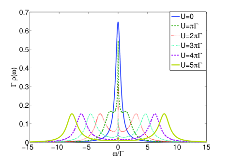
Figure 1: (Color online) Equilibrium density of states in the particle-hole symmetric case at $T/\Gamma=10^{-3}$ for different values of the parameter $U$ (the chemical potential of the lead $\mu_{eq}$ is taken equal to $0$). The density of states for large $U$ shows a three-peak structure with two broad side peaks and a narrow Kondo resonance peak centered at the Fermi level.

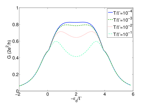
Figure 2: Linear conductance as a function of dot level energy $\varepsilon_{d}$, for $U/\Gamma=4$ and at different temperatures. When the temperature is lowered, the conductance is enhanced in the singly-occupied regime $-\varepsilon_{d}/\Gamma\in[0,4]$, and eventually reaches the maximum conductance $2e^{2}/h$ for a single channel at zero temperature. The conductance does not reach this limit here because of the numerical accuracy of the self-consistent treatment.

IV.2 In equilibrium

We compute the density of states in the dot $\rho_{\sigma}(\omega)=-1/\pi{\rm Im}\mathcal{G}_{\sigma}^{r}(\omega)$ at equilibrium using our EOM approach. Fig.1 reports the result for the density of states at equilibrium and $T/\Gamma=10^{-3}$ for different values of the parameter $U$ when the value of the Fermi level of the leads $\mu_{eq}$ is taken equal to zero. We willingly choose to consider the particle-hole symmetric case ($\varepsilon_{d}=-U/2$) since we know that it is a delicate case in the sense that the EOM approaches developed so far have failed to describe it correctly. The density of states shows a three-peak structure as soon as $U$ becomes larger than $\Gamma$, with two broad peaks and a narrow Kondo resonance peak. The two broad peaks are centered at the renormalized energy levels; their position, intensity and amplitude agree quantitatively with the NRG resultCosti90 . The Kondo resonance peak is pinned at the Fermi level of the leads.

The fact that our EOM scheme correctly describes the particle-hole symmetric case is one of the successes of the method. This can be understood by the fact that in the previous EOM approaches, for the Kondo regime, there is an exact cancellation of the divergent terms $Q_{\bar{\sigma}}(\omega_{{\bar{\sigma}}:\sigma})-Q_{\bar{\sigma}}(-\omega_{:\sigma{\bar{\sigma}}}+U)=Q_{\bar{\sigma}}(\omega)-Q_{\bar{\sigma}}(-\omega)=0$. This feature is cured in our EOM approach since the function $Q_{\bar{\sigma}}(-\omega_{:\sigma{\bar{\sigma}}}+U)$ in Eq. (26) acquires a finite transition rate $2\Gamma$ and is therefore smeared out. Therefore, the cancellation does not occur any longer, and we are left with a divergence in the self-energy at the origin of the formation of the Kondo resonance peak. Through the same argument, our approach is shown in Sec.III.2.3 to improve the prediction made previously by the Lacroix approximation for the Kondo temperature in the particle-hole symmetric case.

Moreover, the density of states at the Fermi level is found to be $\rho_{\sigma}(\mu_{eq})=2/\pi\Gamma$ in agreement with the Fermi liquid property at zero temperature and hence respecting the unitarity condition. This can be explained as follows: at zero temperature, the functions $P_{\sigma}(\omega)$ and $Q_{\sigma}(\omega)$ diverge logarithmically as $\omega\rightarrow\mu_{eq}$,

$$P_{\sigma}(\omega)&=-\frac{\Gamma_{\sigma}}{\pi}\mathcal{G}^{a}_{\sigma}(\mu_{eq}){\rm ln}\left|\omega-\mu_{eq}\right|+\mathcal{O}(1),\\ Q_{\sigma}(\omega)=-\frac{\Gamma_{\sigma}}{\pi}[1+i\Gamma_{\sigma}\mathcal{G}^{a}_{\sigma}(\mu_{eq})]{\rm ln}\left|\omega-\mu_{eq}\right|+\mathcal{O}(1).$$ (40)

We find that the inverse of the imaginary part of $\mathcal{G}^{r}_{\sigma}(\omega)$ (cf.Eqs. (17,26)) is ${\rm Im}[\mathcal{G}^{r}_{\sigma}]^{-1}(\mu_{eq})=\Gamma/2$, as expected from the Fermi liquid theory. In the particle-hole symmetric case, we find ${\rm Re}\mathcal{G}^{r}_{\sigma}(\mu_{eq})\simeq 0$. Combining these two results leads to $\rho_{\sigma}(\mu_{eq})=2/\pi\Gamma$ as observed in Fig.1. Inserting the value of $\rho_{\sigma}(\mu_{eq})$ into Eq. (2) allows one to find the current at small bias voltages and from there the linear conductance $G=dI/dV|_{V=0}$. When the dot is symmetrically coupled to the two leads, the unitary limit $G={2e^{2}}/{h}$ is recovered at zero temperature. The numerical results for $G$ as a function of the dot level $\varepsilon_{d}$ are shown in Fig. 2. As can be noticed, the method underestimates $G$ and the unitary limit is not exactly recovered at $\varepsilon_{d}=-U/2$ because of the numerical accuracy of the self-consistent treatment.

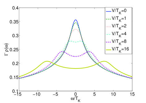
Figure 3: (Color online) Nonequilibrium density of states in the particle-hole symmetric case at $U/\Gamma=4$ and $T/\Gamma=10^{-3}$ for different values of the bias voltage $V$. The chemical potentials of the two leads are taken equal to $\mu_{L/R}=\pm V/2$. The Kondo resonance peak splits into two side peaks located at $\omega=\pm V/2$, i.e. at the positions of the left- and right-lead chemical potentials. For convenience we choose to represent the two energy scales (energy $\omega$ and bias voltage $V$) as normalized by the factor $T_{K}^{-1}$.

IV.3 Out of equilibrium

IV.3.1 Differential conductance

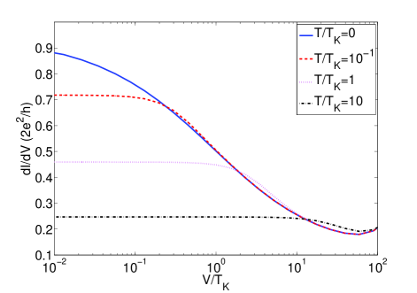
Figure 4: (Color online) Differential conductance $dI/dV$ versus the bias voltage $V$ in the particle-hole symmetric case at $U/\Gamma=4$ for different values of temperature. The curves show a zero-bias peak, followed by the beginning of a broad Coulomb peak at large bias voltage. The differential conductance is reduced when either the temperature or the bias voltage increases, suggesting that the Kondo effect is suppressed by temperature or nonequilibrium effects.

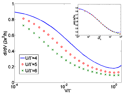
Figure 5: (Color online) Differential conductance $dI/dV$ versus the bias voltage $V$ at $T/T_{K}=0.1$ in the particle-hole symmetric case for different values of $U$. The inset shows that the differential conductance as a function of normalized bias voltage $V/T_{K}$ scales to a single universal curve $dI/dV=f(V/T_{K})$. At higher voltages, the universal behavior is destroyed by a broad peak resulting from charge fluctuations.

Out of equilibrium, the density of states in the dot is greatly influenced by the bias voltage or the difference between the chemical potentials of the leads. Fig. 3 reports our results for the nonequilibrium density of states, again in the particle-hole symmetric case at $T/\Gamma=10^{-3}$ and $U/\Gamma=4$ for different values of the bias voltage $V$. In contrast with the equilibrium situation, the Kondo resonance peak splits into two lower peaks pinned at the chemical potentials of the two leads. The reason is that the transitions between the ground state and the excited states of the dot are now mediated by the conduction electrons with energies lying close to the left- and right-lead chemical potentials.

We then compute the differential conductance as a function of bias voltage for different temperatures and plot the results in Fig. 4. At low temperatures, the bias voltage dependence of the differential conductance shows a narrow peak at low bias (zero-bias anomaly) reflecting the Kondo effect (mind the logarithmic horizontal axis), followed by a Coulomb peak centered around the value of the dot level energy. Increasing temperature diminishes the intensity of the zero-bias peak, meaning that the Kondo effect is destroyed by temperature.

In order to discuss the universality of the dependence of the differential conductance on the bias voltage, we plot in Fig. 5 the results obtained at zero temperature for different values of the Coulomb interaction $U$. In the inset, the differential conductance is found to be a universal function of the renormalized bias voltage $V/T_{K}$, independent of other energy scales such as $U$ or $\Gamma$. This one-parameter scaling is obtained over a large range of $V$. Universality is lost around $V>10T_{K}$. Note that when $V/T_{K}<0.1$, the unitary limit is not completely recovered for the differential conductance due to the numerical accuracy in the self-consistency treatment, as was already mentioned before.

The physical origin of the destruction of the Kondo effect is the decoherence rates induced by the voltage-driven current. As we discussed in Sec.III.2.2, these effects are well described by our EOM approach since it incorporates higher-order terms in $t_{\sigma}$. They originate physically from the energy-conserving processes in which one electron hops onto the dot from the higher chemical potential while another electron hops out to the lower chemical potential. Since the processes involve two electrons hopping in and out, the lowest-order contribution is fourth order in $t_{\sigma}$. These rates broaden and diminish the Kondo resonance peaks in the density of states as the bias voltage increases, see Fig. 3. Their effect leads to a decrease in the differential conductance when $V\geq T_{K}$, as was shown in Figures 4 and 5. We will analyse this in more detail later in this section.

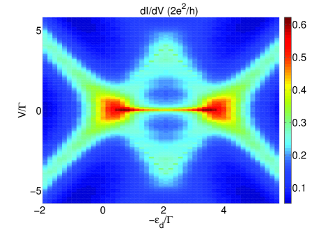
Figure 6: Color plot of the differential conductance $dI/dV$ as a function of bias voltage $V$ and dot-level energy $\varepsilon_{d}$ for $U/\Gamma=4$ and $T/\Gamma=10^{-3}$. The contour of the Coulomb peaks delimits the Coulomb blockade diamond, separating areas with well-defined dot occupation number $\mathcal{N}$ ranging from $0,~{}1$ to $2$ at low $V$, and areas of charge fluctuations at high $V$. In the $\mathcal{N}=1$ central valley, $dI/dV$ shows a zero-bias peak typical of the Kondo effect.

To further demonstrate that the method can work in a wide range of parameters, we report in Fig.6 the differential conductance in the $V-\varepsilon_{d}$ plane in a 3D-plot. The figure shows the usual Coulomb diamond defining inside the Coulomb blockade regime $\mathcal{N}=1$, where $\mathcal{N}$ is the total occupation number in the dot ($\mathcal{N}=\sum_{\sigma}n_{\sigma}$). The boundaries of the Coulomb diamond are related to the values of the renormalized dot level energies $\pm\varepsilon_{d}$ and $\pm\varepsilon_{d}+U$ (with some additional renormalization effects in the mixed valence regime). Within the Coulomb diamond along the $V=0$ line, one can clearly see the zero-bias peak as discussed in Fig. 2. At zero temperature, the unitary limit $2e^{2}/h$ is almost reached at the particle-hole symmetric point ($\varepsilon_{d}=-U/2$). When the temperature is increased, the zero-bias differential conductance decreases at this point, leaving aside two broad Coulomb peaks corresponding to the alignment of the dot level energy with the chemical potentials in the leads ($\varepsilon_{d}=-U$ and $\varepsilon_{d}=0$).

IV.3.2 Comparison with other studies

We compare our results for the differential conductance with those obtained by other groups using time-dependent Numerical Renormalisation GroupAnders2008 and an imaginary-time theory solved by using Quantum Monte CarloHanHeary2007 ; Han2009 , and plot the results obtained for the bias voltage dependence of the differential conductance at zero temperature for comparison (Fig. 7).

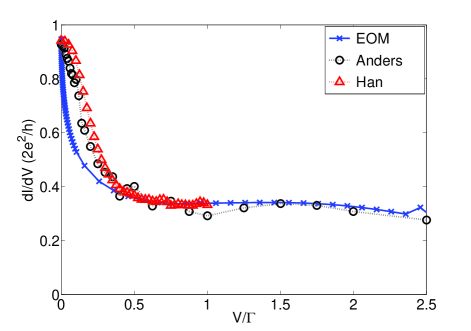
Figure 7: Comparison of the differential conductance $dI/dV$ as a function of bias voltage $V$ with the results obtained by AndersAnders2008 and HanHan2009 for $-2\varepsilon_{d}/\Gamma=U/\Gamma=2.5$ and $T/\Gamma=0.008\ll T_{K}/\Gamma$ (We are grateful to J.E. Han for providing us with his data points). Our curve is plotted for $T=0$ in order to compare the three results in the strong coupling regime. $dI/dV$ at small $V$ is slightly different in the EOM approach because its value for $T_{K}$ is smaller. At high bias voltage, the results of the three approaches agree perfectly. A little unphysical bump is observed for the EOM result at $V=U=2.5\Gamma$, when the chemical potentials of the leads are aligned with the resonant levels of the dot ($\mu_{L}=\varepsilon_{d}+U$, $\mu_{R}=\varepsilon_{d}$).

One finds a qualitative agreement at low bias voltages, when the system is in the strong coupling regime. In that regime, our method slightly underestimates $dI/dV$ because it gives a smaller Kondo scale. The three curves join at higher bias voltages, where a quantitative agreement is found. A little local bump is observed for the EOM result at $V=U$, when the chemical potentials of the leads are aligned with the resonant levels of the dot ($\mu_{L}=\varepsilon_{d}+U$, $\mu_{R}=\varepsilon_{d}$). This is related to the fact that we used the bare $D_{\sigma}(\varepsilon)$ functions (32) in the non-Kondo regime, leading to divergence at $\mu_{L(R)}=\left\{\varepsilon_{d},\varepsilon_{d}+U\right\}$. This bump can be smeared out by introducing a finite width of order $\Gamma$ into the $D_{\sigma}(\varepsilon)$ functions, as can be physically originated from charge fluctuations on the dot resonant levels.

IV.3.3 Crossover from strong coupling to weak coupling regime

When a bias voltage is applied to the leads, it is interesting to know whether or not the decoherence effects induced by the voltage-driven current (cf. Sec.III.2.2) may drive the system from strong to weak coupling regime. We point out that this problem has been discussed in previous studies for the Kondo model using either a perturbative renormalization approachColeman2001 or a slave-boson technique within non-crossing approximationRosch2001 . We would like to tackle this question for the Anderson model with two leads using the EOM scheme.

At zero temperature and at $V\gg T_{K}$, $\mathcal{G}^{r}_{\sigma}(\omega)$ for the Kondo regime behaves as

$$\mathcal{G}^{r}_{\sigma}(\omega)\propto\left[{\rm ln}\left(\frac{(\omega-V/2+i\gamma^{(4)})(\omega+V/2+i\gamma^{(4)})}{T^{2}_{K}}\right)\right]^{-1},$$ (41)

where $\gamma^{(4)}$ is the decoherence rate induced by the bias voltage as given by Eq. (31). $\mathcal{G}^{r}_{\sigma}(\omega)$ given by Eq. (41) develops a poleRosch2001 as soon as $\gamma^{(4)}$ is smaller than a characteristic energy scale $T^{*}$

$$T^{*}=\left\{\begin{array}[]{r@{\quad:\quad}l}\sqrt{T_{K}^{2}-V^{2}/4}&V<\sqrt{2}\,T_{K}\\ T_{K}^{2}/V&V>\sqrt{2}\,T_{K}\end{array}\right.$$ (44)

From there, we define a criterion controlling the crossover between strong coupling ($\gamma^{(4)}<T^{*}$) and weak coupling ($\gamma^{(4)}>T^{*}$) regime, as proposed in Ref.Rosch2001, . In order to obtain the nontrivial decoherence rate $\gamma^{(4)}$ as a function of bias voltage $V$, we replace $D_{\sigma}(\varepsilon)$ of the bare $J_{\alpha\sigma,\beta\sigma^{\prime}}$ in the decoherence rate by the ‘dressed’ $\widetilde{D}_{\sigma}(\varepsilon)$, which is identified with the denominator of the Green function (17). Thus we can define a renormalized $\widetilde{J}_{\alpha\sigma,\beta\sigma^{\prime}}\equiv 2t_{\alpha\sigma}t_{\beta\sigma^{\prime}}\widetilde{D}_{\sigma}(\mu_{\alpha})$. In the limit $V\gg T_{K}$, we find $\widetilde{J}_{\alpha\sigma,\beta\sigma^{\prime}}\propto 1/[2~{}{\rm ln}(V/T_{K})]$ and $\gamma^{(4)}\propto V/[2~{}{\rm ln}(V/T_{K})]^{2}$, which is always larger than $T^{*}$. The results for the renormalized decoherence rate $\gamma^{(4)}/T_{K}$ as a function of the bias voltage are reported in Fig. 8 for different values of $U$. Strikingly, the curves for the different values of $U$ coincide, underlining the universality of the evolution of $\gamma^{(4)}/T_{K}$ as a function of $V/T_{K}$. Combining the results for $T^{*}/T_{K}$ and $\gamma^{(4)}/T_{K}$, one can derive the universal crossover bias voltage $V_{c}/T_{K}$ from strong to weak coupling regime.

At finite temperatures, the derivation for $T^{*}$ is the same except for replacing $\gamma^{(4)}\rightarrow\sqrt{(\gamma^{(4)})^{2}+\pi^{2}T^{2}}$ in Eq. (41). The results are plotted in Fig. 8 in the $V-T$ plane, displaying the crossover from strong coupling to weak coupling regime. Although the physical mechanism at the origin of the crossover is different, both bias voltage and temperature drive the system to the weak coupling regime.

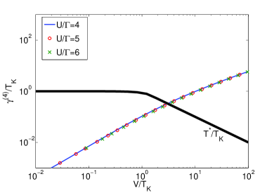
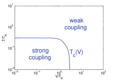
Figure 8: (Color online) (a) Decoherence rate $\gamma^{(4)}$ and characteristic energy scale $T^{*}$ versus the normalized bias voltage $V/T_{K}$ at $T/T_{K}=10^{-1}$ in the particle-hole symmetric case for several values of $U/\Gamma$. $\gamma^{(4)}/T_{K}$ is a universal function of $V/T_{K}$ over a large range of $V$. The comparison of both energy scales ($\gamma^{(4)}$ and $T^{*}$) allows one to determine whether the system is in the strong coupling regime ($\gamma^{(4)}<T^{*}$) or weak coupling regime ($\gamma^{(4)}>T^{*}$). (b) Stability phase diagram of the strong coupling and weak coupling regimes in the $V-T$ plane. The crossover tempeature $T_{c}(V)/T_{K}$ is a universal function of $V/T_{K}$.

IV.3.4 Nonequilibrium occupation number in the dot

Typically, at equilibrium and for zero temperature, $\langle n_{\sigma}\rangle$ is mainly determined by the weight of the broad resonance peak far below the Fermi level. The narrow Kondo resonance near the Fermi energy has little weight in comparison. Thus, even if a EOM approach in a certain approximation scheme happens to describe only qualitatively Kondo physics, it is able to determine numerically the occupation number that agrees reasonably well with the Bethe ansatz or NRG.

When the system is driven out of equilibrium, the problem becomes more complicated as one should use lesser Green functions instead of retarded ones to compute the expectation values. As discussed in Sec.IV.1, the only place where this cannot be circumvented is precisely for the dot occupation number $\langle n_{\sigma}\rangle$ appearing in the Green function (17). A rigorous treatment would require to compute the lesser Green function $\mathcal{G}^{<}_{\sigma}(\omega)$ and then obtain $\langle n_{\sigma}\rangle$ according to Eq. (39), which is beyond the scope of this work. As described in Sec.IV.1, we used instead the Ng ansatz to compute the dot occupation number. On the other hand, if we consider the particle-hole symmetric case ($\varepsilon_{d}=-U/2$), with a symmetric bias voltage setting $[\mu_{L},\mu_{R}]=[V/2,-V/2]$, one obtains $\langle n_{\sigma}\rangle=1/2$ by symmetry. However, we noticed that the calculation of the occupation number by applying the Ng ansatz to our Green function leads to slight deviation from $\langle n_{\sigma}\rangle=1/2$. In Appendix IV, we show how to solve this problem.

On the other hand, for an asymmetric bias voltage setting, the occupation number $\langle n_{\sigma}\rangle$ is no longer fixed by symmetry arguments. Let us take $[\mu_{L},\mu_{R}]=[0,-V]$, the bias voltage dependence of the occupation number is shown in Fig. 9. As $V$ increases, $\langle n_{\sigma}\rangle$ decreases rapidly till $V$ passes the dot-level energy $U/2$ and comes to stabilize at large $V$. This can be qualitatively explained by the fact that at large $V$, the current through the dot no longer increases monotonously with the bias voltage and reaches a horizontal asymptote. This makes the occupation number insensitive to the bias voltage.

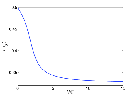
Figure 9: (Color online) Occupation number in the dot $\langle n_{\sigma}\rangle$ versus the bias voltage $V$ in the particle-hole symmetric case for $U/\Gamma$ and $T/\Gamma=8.510^{-4}$, and under an asymmetric bias voltage setting $\mu_{L}=0$ and $\mu_{R}=-V$.

V Conclusions

We have presented a study of the nonequilibrium effects in the two-lead Anderson model. The calculations have been performed within a self-consistent EOM approach generalized to the nonequilibrium situation. The approximation scheme presented in this paper goes beyond the previous truncations of the equations of motion done at the second or fourth order in tunneling $t_{\sigma}$, by including contributions from the next orders (sixth order), which have been shown to be of great importance out of equilibrium.

The situation at equilibrium is used as a benchmark for the approximation. The results for the density of states and the linear conductance at equilibrium are found to be quantitatively improved compared to those obtained by the EOM method using the Lacroix approximation. In the Kondo regime for instance, the Kondo temperature $T_{K}$ is closer to the exact results found with the Bethe ansatz and NRG, and non longer vanishes in the particle-hole symmetric case. When the dot is symmetrically coupled to the leads, the linear conductance reaches its unitary limit $2e^{2}/h$ at zero temperature in the Kondo regime.

We have also computed the nonequilibrium decoherence rate $\gamma^{(4)}$ in the Kondo regime. At $T\gg T_{K}$, $\gamma^{(4)}/T_{K}$ is found to be a universal increasing function of the normalized bias voltage $V/T_{K}$, depending on a single energy scale $T_{K}$. The scaling law holds over a wide range of $V$ going from $0$ to $100T_{K}$. At low temperature, the density of states shows a splitting of the Kondo resonance into two peaks, pinned at the chemical potentials of the two leads. The height of the two peaks is controlled by the decoherence rate.

As far as the differential conductance is concerned, it shows a zero-bias peak at low temperature, followed by a broad Coulomb peak at larger bias voltage. At low bias voltage, the differential conductance also obeys a universal scaling law as a function of $V/T_{K}$. Finally we have discussed the role played by the decoherence rate $\gamma^{(4)}$ in driving the system from the strong coupling to the weak coupling regime. We have derived the crossover line $T_{c}(V)$ separating the strong coupling regime to the weak coupling regime.

Appendix I Derivation of equations of motion for finite Coulomb interaction

Appendix I.1

In Section II, we have derived the first equations of motion. In this appendix, we present the detailed derivation of the higher hierarchy of equations and the decoupling scheme that follows. We derive the EOM of the higher Green functions on the right-hand side of Eq. (8) by using Eq. (4). They are

$$\omega_{:k}\langle\langle n_{\bar{\sigma}}c_{k\sigma}\rangle\rangle&=t_{\sigma}\langle\langle n_{\bar{\sigma}}f_{\sigma}\rangle\rangle+\sum_{k^{\prime}}t_{\bar{\sigma}}\Big{[}\langle\langle f_{\bar{\sigma}}^{{\dagger}}c_{k^{\prime}{\bar{\sigma}}}c_{k\sigma}\rangle\rangle-\langle\langle c_{k^{\prime}{\bar{\sigma}}}^{{\dagger}}f_{\bar{\sigma}}c_{k\sigma}\rangle\rangle\Big{]},\\ \omega_{{\bar{\sigma}}:\sigma k}\langle\langle f_{\bar{\sigma}}^{{\dagger}}c_{k{\bar{\sigma}}}f_{\sigma}\rangle\rangle=\langle f_{\bar{\sigma}}^{{\dagger}}c_{k{\bar{\sigma}}}\rangle+t_{{\bar{\sigma}}}\langle\langle n_{\bar{\sigma}}f_{\sigma}\rangle\rangle+\sum_{k^{\prime}}\Big{[}t_{\sigma}\langle\langle f_{\bar{\sigma}}^{{\dagger}}c_{k{\bar{\sigma}}}c_{k^{\prime}\sigma}\rangle\rangle-t_{{\bar{\sigma}}}\langle\langle c_{k^{\prime}{\bar{\sigma}}}^{{\dagger}}c_{k{\bar{\sigma}}}f_{\sigma}\rangle\rangle\Big{]},\\ \left(\omega_{k:\sigma{\bar{\sigma}}}-U\right)\langle\langle c_{k{\bar{\sigma}}}^{{\dagger}}f_{\bar{\sigma}}f_{\sigma}\rangle\rangle=\langle c_{k{\bar{\sigma}}}^{{\dagger}}f_{\bar{\sigma}}\rangle-t_{\bar{\sigma}}\langle\langle n_{\bar{\sigma}}f_{\sigma}\rangle\rangle+\sum_{k^{\prime}}\Big{[}t_{\bar{\sigma}}\langle\langle c_{k{\bar{\sigma}}}^{{\dagger}}c_{k^{\prime}{\bar{\sigma}}}f_{\sigma}\rangle\rangle+t_{\sigma}\langle\langle c_{k{\bar{\sigma}}}^{{\dagger}}f_{\bar{\sigma}}c_{k^{\prime}\sigma}\rangle\rangle\Big{]},$$ (A.1)

where we denote for a shorthand

$$\omega_{\alpha\beta\cdots:ab\cdots} \equiv \omega+\varepsilon_{\alpha}+\varepsilon_{\beta}+\cdots-\varepsilon_{a}-\varepsilon_{b}-\cdots,$$

with $\left\{\alpha\beta\cdots,ab\cdots\right\}$ being any set of parameters within $k$’s and $\sigma$’s.

For most practical purposes, the truncation is performed at this level by decoupling the second-order terms on the right-hand side of Eqs. (A.1), see the paragraph in the main text after Eqs. (10). This is done by grouping all possible same-spin pairs of lead ($c$) and dot ($f$) electron operators since we assume the spin quantum number is preserved through tunneling: any correlation between electrons of different spins has to come via the Coulomb interaction. A solution obtained at this level by neglecting the connected Green functions is exact to second order in hybridizationKashcheyevs2006 . Numerous such solutions can be found in the literatureLacroix1981 ; MWL1991 ; Appelbaum1969 ; Wohlman2005 , with some more elaborate than the others.

However, as discussed in the main text, stopping the flow at this point will raise terms suffering from logarithmic divergences. In the following, we show how to go beyond the second-order to derive higher equations of motion exact up to the fourth order. To begin with, we consider the following second-generation EOM:

$$\omega_{{\bar{\sigma}}:k{k^{\prime}}}\langle\langle f_{\bar{\sigma}}^{{\dagger}}c_{k^{\prime}{\bar{\sigma}}}c_{k\sigma}\rangle\rangle&=-U\langle\langle n_{\sigma}f_{\bar{\sigma}}^{{\dagger}}c_{k^{\prime}{\bar{\sigma}}}c_{k\sigma}\rangle\rangle+t_{\bar{\sigma}}\langle\langle n_{\bar{\sigma}}c_{k\sigma}\rangle\rangle+t_{\sigma}\langle\langle f_{\bar{\sigma}}^{{\dagger}}c_{k^{\prime}{\bar{\sigma}}}f_{\sigma}\rangle\rangle-\sum_{{k^{\prime\prime}}}t_{\bar{\sigma}}\langle\langle c_{{k^{\prime\prime}}{\bar{\sigma}}}^{{\dagger}}c_{k^{\prime}{\bar{\sigma}}}c_{k\sigma}\rangle\rangle,\\ \omega_{{k^{\prime}}:\sigma k}\langle\langle c_{k^{\prime}{\bar{\sigma}}}^{{\dagger}}c_{k{\bar{\sigma}}}f_{\sigma}\rangle\rangle=f_{{k^{\prime}}k}^{\bar{\sigma}}+U\langle\langle n_{\bar{\sigma}}c_{k^{\prime}{\bar{\sigma}}}^{{\dagger}}c_{k{\bar{\sigma}}}f_{\sigma}\rangle\rangle+t_{\bar{\sigma}}\langle\langle c_{k^{\prime}{\bar{\sigma}}}^{{\dagger}}f_{{\bar{\sigma}}}f_{\sigma}\rangle\rangle-t_{\bar{\sigma}}\langle\langle f_{{\bar{\sigma}}}^{{\dagger}}c_{k{\bar{\sigma}}}f_{\sigma}\rangle\rangle+\sum_{k^{\prime\prime}}t_{\sigma}\langle\langle c_{k^{\prime}{\bar{\sigma}}}^{{\dagger}}c_{k{\bar{\sigma}}}c_{{k^{\prime\prime}}\sigma}\rangle\rangle,\\ \omega_{{k^{\prime}}:{\bar{\sigma}}k}\langle\langle c_{k^{\prime}{\bar{\sigma}}}^{{\dagger}}f_{{\bar{\sigma}}}c_{k\sigma}\rangle\rangle=U\langle\langle n_{\sigma}c_{k^{\prime}{\bar{\sigma}}}^{{\dagger}}f_{{\bar{\sigma}}}c_{k\sigma}\rangle\rangle-t_{\bar{\sigma}}\langle\langle n_{\bar{\sigma}}c_{k\sigma},f_{\sigma}^{{\dagger}}\rangle\rangle+t_{\sigma}\langle\langle c_{k^{\prime}{\bar{\sigma}}}^{{\dagger}}f_{{\bar{\sigma}}}f_{\sigma}\rangle\rangle+\sum_{k^{\prime\prime}}t_{\bar{\sigma}}\langle\langle c_{k^{\prime}{\bar{\sigma}}}^{{\dagger}}c_{{k^{\prime\prime}}{\bar{\sigma}}}c_{k\sigma}\rangle\rangle.$$ (A.2)

where we denote $f_{{k^{\prime}}k}^{\sigma}\equiv\langle c_{{k^{\prime}}\sigma}^{\dagger}c_{k\sigma}\rangle.$

We proceed to insert the above Eqs. (A.2) into Eqs. (A.1). The right-hand side of the latter equations involve new Green functions generated via the Coulomb interaction and others of the same hierarchy as the left-hand side. The latter Green functions can either move to the left-hand side or vanish in the wide-band limit since upon summing over $k$, all denominators have poles in the upper half complex plane. Furthermore, we decouple $\langle\langle c^{\dagger}_{\bar{\sigma}}c_{\bar{\sigma}}c_{\sigma}\rangle\rangle\approx\langle c^{\dagger}_{\bar{\sigma}}c_{\bar{\sigma}}\rangle\langle\langle c_{\sigma}\rangle\rangle$ and then use Eq. (6), since this decoupling should be exact up to order of $t_{\sigma}^{4}$ and for another reason which will be clear later. We end up with

$$\left[\omega_{:k}-\Sigma_{1\sigma}(\omega_{:k})\right]\langle\langle n_{\bar{\sigma}}c_{k\sigma}\rangle\rangle&=t_{\sigma}\langle\langle n_{\bar{\sigma}}f_{\sigma}\rangle\rangle-U\sum_{k^{\prime}}t_{\bar{\sigma}}\left[\omega_{{\bar{\sigma}}:k{k^{\prime}}}^{-1}\langle\langle n_{\sigma}f_{\bar{\sigma}}^{{\dagger}}c_{k^{\prime}{\bar{\sigma}}}c_{k\sigma}\rangle\rangle+\omega_{{k^{\prime}}:{\bar{\sigma}}k}^{-1}\langle\langle n_{\sigma}c_{k^{\prime}{\bar{\sigma}}}^{{\dagger}}f_{{\bar{\sigma}}}c_{k\sigma}\rangle\rangle\right],\\ \left[\omega_{{\bar{\sigma}}:\sigma k}-\Sigma_{2\sigma}(\omega_{:k})\right]\langle\langle f_{\bar{\sigma}}^{{\dagger}}c_{k{\bar{\sigma}}}f_{\sigma}\rangle\rangle=\langle f_{\bar{\sigma}}^{{\dagger}}c_{k{\bar{\sigma}}}\rangle+t_{{\bar{\sigma}}}\langle\langle n_{\bar{\sigma}}f_{\sigma}\rangle\rangle-\sum_{k^{\prime}}t_{\bar{\sigma}}\omega_{{k^{\prime}}:\sigma k}^{-1}f_{{k^{\prime}}k}^{\bar{\sigma}}\left[1+\Sigma^{0}_{\sigma}(\omega)\langle\langle f_{\sigma}\rangle\rangle\right]\\ -U\sum_{k^{\prime}}\left[t_{\sigma}\omega_{{\bar{\sigma}}:k{k^{\prime}}}^{-1}\langle\langle n_{\sigma}f_{\bar{\sigma}}^{{\dagger}}c_{k{\bar{\sigma}}}c_{{k^{\prime}}\sigma}\rangle\rangle+t_{\bar{\sigma}}\omega_{{k^{\prime}}:\sigma k}^{-1}\langle\langle n_{\bar{\sigma}}c_{k^{\prime}{\bar{\sigma}}}^{{\dagger}}c_{k{\bar{\sigma}}}f_{\sigma}\rangle\rangle\right],\\ \left[\omega_{k:\sigma{\bar{\sigma}}}-U-\Sigma_{3\sigma}(\omega_{k:})\right]\langle\langle c_{k{\bar{\sigma}}}^{{\dagger}}f_{\bar{\sigma}}f_{\sigma}\rangle\rangle=\langle c_{k{\bar{\sigma}}}^{{\dagger}}f_{\bar{\sigma}}\rangle-t_{\bar{\sigma}}\langle\langle n_{\bar{\sigma}}f_{\sigma}\rangle\rangle+\sum_{k^{\prime}}t_{\bar{\sigma}}\omega_{k:\sigma{k^{\prime}}}^{-1}f_{k{k^{\prime}}}^{\bar{\sigma}}\left[1+\Sigma^{0}_{\sigma}(\omega)\langle\langle f_{\sigma}\rangle\rangle\right]\\ +U\sum_{k^{\prime}}\left[t_{\sigma}\omega_{k:{\bar{\sigma}}{k^{\prime}}}^{-1}\langle\langle n_{\sigma}c_{k{\bar{\sigma}}}^{{\dagger}}f_{\bar{\sigma}}c_{{k^{\prime}}\sigma}\rangle\rangle+t_{\bar{\sigma}}\omega_{k:\sigma{k^{\prime}}}^{-1}\langle\langle n_{\bar{\sigma}}c_{k{\bar{\sigma}}}^{{\dagger}}c_{{k^{\prime}}{\bar{\sigma}}}f_{\sigma}\rangle\rangle\right].$$ (A.3)

where

$$\Sigma^{0}_{\sigma}(\omega) = \sum_{k}t_{\sigma}^{2}\omega_{:k}^{-1},$$ (A.4)

$$\Sigma_{1\sigma}(\omega_{:k}) = \sum_{{k^{\prime}}}t_{\bar{\sigma}}^{2}\left[\omega_{{\bar{\sigma}}:k{k^{\prime}}}^{-1}+\omega_{{k^{\prime}}:{\bar{\sigma}}k}^{-1}\right],$$ (A.5)

$$\Sigma_{2\sigma}(\omega_{:k}) = \sum_{{k^{\prime}}}\left[t_{\sigma}^{2}\omega_{{\bar{\sigma}}:k{k^{\prime}}}^{-1}+t_{\bar{\sigma}}^{2}\omega_{{k^{\prime}}:\sigma k}^{-1}\right],$$ (A.6)

$$\Sigma_{3\sigma}(\omega_{k:}) = \sum_{{k^{\prime}}}\left[t_{\bar{\sigma}}^{2}\omega_{k:\sigma{k^{\prime}}}^{-1}+t_{\sigma}^{2}\omega_{k:{\bar{\sigma}}{k^{\prime}}}^{-1}\right].$$ (A.7)

It is interesting to notice that at this level the prefactor of the Green functions on the left-hand side acquires non-interacting self-energy terms, while new Green functions remain on the right-hand side. This allows us to focus on the new Green functions, which is of most importance.  We list below these third-generation equations of motion,

$$\left(\omega_{{\bar{\sigma}}:{k^{\prime}}k}+U\right)\langle\langle n_{\sigma}f_{\bar{\sigma}}^{{\dagger}}c_{k{\bar{\sigma}}}c_{{k^{\prime}}\sigma}\rangle\rangle&=-\langle f_{\bar{\sigma}}^{{\dagger}}c_{k{\bar{\sigma}}}f_{\sigma}^{{\dagger}}c_{{k^{\prime}}\sigma}\rangle+t_{\bar{\sigma}}\langle\langle n_{\sigma}n_{\bar{\sigma}}c_{{k^{\prime}}\sigma}\rangle\rangle-\sum_{k^{\prime\prime}}t_{\sigma}\langle\langle c_{{k^{\prime\prime}}\sigma}^{\dagger}f_{\sigma}f_{\bar{\sigma}}^{{\dagger}}c_{k{\bar{\sigma}}}c_{{k^{\prime}}\sigma}\rangle\rangle\\ +\sum_{k^{\prime\prime}}t_{\sigma}\langle\langle f_{\sigma}^{\dagger}c_{{k^{\prime\prime}}\sigma}f_{\bar{\sigma}}^{{\dagger}}c_{k{\bar{\sigma}}}c_{{k^{\prime}}\sigma}\rangle\rangle-\sum_{k^{\prime\prime}}t_{\bar{\sigma}}\langle\langle n_{\sigma}c_{{k^{\prime\prime}}{\bar{\sigma}}}^{\dagger}c_{k{\bar{\sigma}}}c_{{k^{\prime}}\sigma}\rangle\rangle,\\ \left(\omega_{{k^{\prime}}:{\bar{\sigma}}k}-U\right)\langle\langle n_{\sigma}c_{k^{\prime}{\bar{\sigma}}}^{{\dagger}}f_{{\bar{\sigma}}}c_{k\sigma}\rangle\rangle=-\langle c_{k^{\prime}{\bar{\sigma}}}^{{\dagger}}f_{{\bar{\sigma}}}f_{\sigma}^{{\dagger}}c_{k\sigma}\rangle-t_{\bar{\sigma}}\langle\langle n_{\sigma}n_{\bar{\sigma}}c_{k\sigma}\rangle\rangle-\sum_{k^{\prime\prime}}t_{\sigma}\langle\langle c_{{k^{\prime\prime}}\sigma}^{\dagger}f_{\sigma}c_{k^{\prime}{\bar{\sigma}}}^{{\dagger}}f_{{\bar{\sigma}}}c_{k\sigma}\rangle\rangle\\ +\sum_{k^{\prime\prime}}t_{\sigma}\langle\langle f_{\sigma}^{\dagger}c_{{k^{\prime\prime}}\sigma}c_{k^{\prime}{\bar{\sigma}}}^{{\dagger}}f_{{\bar{\sigma}}}c_{k\sigma}\rangle\rangle+\sum_{k^{\prime\prime}}t_{\bar{\sigma}}\langle\langle n_{\sigma}c_{k^{\prime}{\bar{\sigma}}}^{{\dagger}}c_{{k^{\prime\prime}}{\bar{\sigma}}}c_{k\sigma}\rangle\rangle,\\ \left(\omega_{{k^{\prime}}:\sigma k}-U\right)\langle\langle n_{\bar{\sigma}}c_{k^{\prime}{\bar{\sigma}}}^{{\dagger}}c_{k{\bar{\sigma}}}f_{\sigma}\rangle\rangle=\langle n_{\bar{\sigma}}c_{k^{\prime}{\bar{\sigma}}}^{{\dagger}}c_{k{\bar{\sigma}}}\rangle-\sum_{k^{\prime\prime}}t_{\bar{\sigma}}\langle\langle c_{{k^{\prime\prime}}{\bar{\sigma}}}^{\dagger}f_{\bar{\sigma}}c_{k^{\prime}{\bar{\sigma}}}^{{\dagger}}c_{k{\bar{\sigma}}}f_{\sigma}\rangle\rangle\\ -\sum_{k^{\prime\prime}}t_{\bar{\sigma}}\langle\langle f_{\bar{\sigma}}^{\dagger}c_{k^{\prime}{\bar{\sigma}}}^{{\dagger}}c_{{k^{\prime\prime}}{\bar{\sigma}}}c_{k{\bar{\sigma}}}f_{\sigma}\rangle\rangle+\sum_{k^{\prime\prime}}t_{\sigma}\langle\langle n_{\bar{\sigma}}c_{k^{\prime}{\bar{\sigma}}}^{{\dagger}}c_{k{\bar{\sigma}}}c_{{k^{\prime\prime}}\sigma}\rangle\rangle.$$ (A.8)

Up to order $t_{\sigma}^{4}$, we decouple Eqs. (A.8) by considering the following decouplings:

$$\langle f_{\bar{\sigma}}^{{\dagger}}c_{k{\bar{\sigma}}}f_{\sigma}^{{\dagger}}c_{{k^{\prime}}\sigma}\rangle&\approx\langle f_{\bar{\sigma}}^{{\dagger}}c_{k{\bar{\sigma}}}\rangle\langle f_{\sigma}^{{\dagger}}c_{{k^{\prime}}\sigma}\rangle,\\ \langle n_{\bar{\sigma}}c_{k^{\prime}{\bar{\sigma}}}^{{\dagger}}c_{k{\bar{\sigma}}}\rangle\approx\langle n_{\bar{\sigma}}\rangle f_{{k^{\prime}}k}^{\bar{\sigma}}-\langle f_{\bar{\sigma}}^{\dagger}c_{k{\bar{\sigma}}}\rangle\langle c_{{k^{\prime}}{\bar{\sigma}}}^{\dagger}f_{\bar{\sigma}}\rangle,\\ \langle c_{{k^{\prime}}{\bar{\sigma}}}^{{\dagger}}f_{{\bar{\sigma}}}f_{\sigma}^{{\dagger}}c_{k\sigma}\rangle\approx\langle c_{k^{\prime}{\bar{\sigma}}}^{{\dagger}}f_{{\bar{\sigma}}}\rangle\langle f_{\sigma}^{{\dagger}}c_{k\sigma}\rangle,\\ \langle\langle c_{{k^{\prime\prime}}\sigma}^{\dagger}f_{\sigma}f_{\bar{\sigma}}^{{\dagger}}c_{k{\bar{\sigma}}}c_{{k^{\prime}}\sigma}\rangle\rangle\approx-f_{{k^{\prime\prime}}{k^{\prime}}}^{\sigma}\langle\langle f_{\bar{\sigma}}^{{\dagger}}c_{k{\bar{\sigma}}}f_{\sigma}\rangle\rangle-\langle f_{\bar{\sigma}}^{{\dagger}}c_{k{\bar{\sigma}}}\rangle\langle\langle c_{{k^{\prime\prime}}\sigma}^{\dagger}c_{{k^{\prime}}\sigma}f_{\sigma}\rangle\rangle+f_{{k^{\prime\prime}}{k^{\prime}}}^{\sigma}\langle f_{\bar{\sigma}}^{{\dagger}}c_{k{\bar{\sigma}}}\rangle\langle\langle f_{\sigma}\rangle\rangle,\\ \langle\langle f_{\sigma}^{\dagger}c_{{k^{\prime\prime}}\sigma}f_{\bar{\sigma}}^{{\dagger}}c_{k{\bar{\sigma}}}c_{{k^{\prime}}\sigma}\rangle\rangle\approx\langle f_{\bar{\sigma}}^{{\dagger}}c_{k{\bar{\sigma}}}\rangle\langle\langle f_{\sigma}^{\dagger}c_{{k^{\prime\prime}}\sigma}c_{{k^{\prime}}\sigma}\rangle\rangle,\\ \langle\langle n_{\sigma}c_{{k^{\prime\prime}}{\bar{\sigma}}}^{\dagger}c_{k{\bar{\sigma}}}c_{{k^{\prime}}\sigma}\rangle\rangle\approx f_{{k^{\prime\prime}}k}^{\bar{\sigma}}\langle\langle n_{\sigma}c_{{k^{\prime}}\sigma}\rangle\rangle,\\ \langle\langle c_{{k^{\prime\prime}}\sigma}^{\dagger}f_{\sigma}c_{k^{\prime}{\bar{\sigma}}}^{{\dagger}}f_{{\bar{\sigma}}}c_{k\sigma}\rangle\rangle\approx-f_{{k^{\prime\prime}}k}^{\sigma}\langle\langle c_{k^{\prime}{\bar{\sigma}}}^{{\dagger}}f_{{\bar{\sigma}}}f_{\sigma}\rangle\rangle-\langle c_{k^{\prime}{\bar{\sigma}}}^{{\dagger}}f_{{\bar{\sigma}}}\rangle\langle\langle c_{{k^{\prime\prime}}\sigma}^{\dagger}c_{k\sigma}f_{\sigma}\rangle\rangle+f_{{k^{\prime\prime}}k}^{\sigma}\langle c_{k^{\prime}{\bar{\sigma}}}^{{\dagger}}f_{{\bar{\sigma}}}\rangle\langle\langle f_{\sigma}\rangle\rangle,\\ \langle\langle f_{\sigma}^{\dagger}c_{{k^{\prime\prime}}\sigma}c_{k^{\prime}{\bar{\sigma}}}^{{\dagger}}f_{{\bar{\sigma}}}c_{k\sigma}\rangle\rangle\approx\langle c_{k^{\prime}{\bar{\sigma}}}^{{\dagger}}f_{{\bar{\sigma}}}\rangle\langle\langle f_{\sigma}^{\dagger}c_{{k^{\prime\prime}}\sigma}c_{k\sigma}\rangle\rangle,\\ \langle\langle c_{{k^{\prime\prime}}{\bar{\sigma}}}^{\dagger}f_{\bar{\sigma}}c_{k^{\prime}{\bar{\sigma}}}^{{\dagger}}c_{k{\bar{\sigma}}}f_{\sigma}\rangle\rangle\approx-f_{{k^{\prime\prime}}k}^{\bar{\sigma}}\langle\langle c_{k^{\prime}{\bar{\sigma}}}^{{\dagger}}f_{\bar{\sigma}}f_{\sigma}\rangle\rangle+f_{{k^{\prime}}k}^{\bar{\sigma}}\langle\langle c_{{k^{\prime\prime}}{\bar{\sigma}}}^{\dagger}f_{\bar{\sigma}}f_{\sigma}\rangle\rangle,\\ \langle\langle f_{\bar{\sigma}}^{\dagger}c_{k^{\prime}{\bar{\sigma}}}^{{\dagger}}c_{{k^{\prime\prime}}{\bar{\sigma}}}c_{k{\bar{\sigma}}}f_{\sigma}\rangle\rangle\approx f_{{k^{\prime}}{k^{\prime\prime}}}^{\bar{\sigma}}\langle\langle f_{\bar{\sigma}}^{\dagger}c_{k{\bar{\sigma}}}f_{\sigma}\rangle\rangle-f_{{k^{\prime}}k}^{\bar{\sigma}}\langle\langle f_{\bar{\sigma}}^{\dagger}c_{{k^{\prime\prime}}{\bar{\sigma}}}f_{\sigma}\rangle\rangle,\\ \langle\langle n_{\bar{\sigma}}c_{k^{\prime}{\bar{\sigma}}}^{{\dagger}}c_{k{\bar{\sigma}}}c_{{k^{\prime\prime}}\sigma}\rangle\rangle\approx f_{{k^{\prime}}k}^{\bar{\sigma}}\langle\langle n_{\bar{\sigma}}c_{{k^{\prime\prime}}\sigma}\rangle\rangle-\langle f_{\bar{\sigma}}^{\dagger}c_{k{\bar{\sigma}}}\rangle\langle\langle c_{{k^{\prime}}{\bar{\sigma}}}^{\dagger}f_{\bar{\sigma}}c_{{k^{\prime\prime}}\sigma}\rangle\rangle.$$ (A.9)

Note that the last terms in Eqs. (A.9, A.9) are added in order to avoid double counting from the first two terms. On the other hand, since $\langle\langle n_{\bar{\sigma}}n_{\sigma}c_{k\sigma}\rangle\rangle$ vanish in the wide-band limit after summing over $k$, they are removed from now on without further notice. Eqs. (A.8) then become

$$(\omega_{{\bar{\sigma}}:{k^{\prime}}k}+U)\langle\langle n_{\sigma}f_{\bar{\sigma}}^{{\dagger}}c_{k{\bar{\sigma}}}c_{{k^{\prime}}\sigma}\rangle\rangle&=\sum_{k^{\prime\prime}}t_{\sigma}f_{{k^{\prime\prime}}{k^{\prime}}}^{\sigma}\langle\langle f_{\bar{\sigma}}^{{\dagger}}c_{k{\bar{\sigma}}}f_{\sigma}\rangle\rangle+\Big{[}\omega_{:{k^{\prime}}}\langle f_{\bar{\sigma}}^{{\dagger}}c_{k{\bar{\sigma}}}\rangle-\sum_{k^{\prime\prime}}t_{\bar{\sigma}}f_{{k^{\prime\prime}}k}^{\bar{\sigma}}\Big{]}\langle\langle n_{\sigma}c_{{k^{\prime}}\sigma}\rangle\rangle\\ -\langle f_{\bar{\sigma}}^{{\dagger}}c_{k{\bar{\sigma}}}\rangle\sum_{k^{\prime\prime}}t_{\sigma}f_{{k^{\prime\prime}}{k^{\prime}}}^{\sigma}\langle\langle f_{\sigma}\rangle\rangle,\\ (\omega_{{k^{\prime}}:{\bar{\sigma}}k}-U)\langle\langle n_{\sigma}c_{k^{\prime}{\bar{\sigma}}}^{{\dagger}}f_{{\bar{\sigma}}}c_{k\sigma}\rangle\rangle=\sum_{k^{\prime\prime}}t_{\sigma}f_{{k^{\prime\prime}}k}^{\sigma}\langle\langle c_{k^{\prime}{\bar{\sigma}}}^{{\dagger}}f_{{\bar{\sigma}}}f_{\sigma}\rangle\rangle+\Big{[}\omega_{:k}\langle c_{k^{\prime}{\bar{\sigma}}}^{{\dagger}}f_{{\bar{\sigma}}}\rangle+\sum_{k^{\prime\prime}}t_{\bar{\sigma}}f_{{k^{\prime}}{k^{\prime\prime}}}^{\bar{\sigma}}\Big{]}\langle\langle n_{\sigma}c_{k\sigma}\rangle\rangle\\ -\langle c_{k^{\prime}{\bar{\sigma}}}^{{\dagger}}f_{{\bar{\sigma}}}\rangle\sum_{k^{\prime\prime}}t_{\sigma}f_{{k^{\prime\prime}}k}^{\sigma}\langle\langle f_{\sigma}\rangle\rangle,\\ (\omega_{{k^{\prime}}:\sigma k}-U)\langle\langle n_{\bar{\sigma}}c_{k^{\prime}{\bar{\sigma}}}^{{\dagger}}c_{k{\bar{\sigma}}}f_{\sigma}\rangle\rangle=-\langle f_{\bar{\sigma}}^{\dagger}c_{k{\bar{\sigma}}}\rangle\Big{[}\langle c_{{k^{\prime}}{\bar{\sigma}}}^{\dagger}f_{\bar{\sigma}}\rangle+\sum_{k^{\prime\prime}}t_{\sigma}\langle\langle c_{{k^{\prime}}{\bar{\sigma}}}^{\dagger}f_{\bar{\sigma}}c_{{k^{\prime\prime}}\sigma}\rangle\rangle\Big{]}+\sum_{k^{\prime\prime}}t_{\bar{\sigma}}f_{{k^{\prime\prime}}k}^{\bar{\sigma}}\langle\langle c_{k^{\prime}{\bar{\sigma}}}^{{\dagger}}f_{\bar{\sigma}}f_{\sigma}\rangle\rangle\\ -\sum_{k^{\prime\prime}}t_{\bar{\sigma}}f_{{k^{\prime}}{k^{\prime\prime}}}^{\bar{\sigma}}\langle\langle f_{\bar{\sigma}}^{\dagger}c_{k{\bar{\sigma}}}f_{\sigma}\rangle\rangle+(\omega_{:\sigma}-U)f_{{k^{\prime}}k}^{\bar{\sigma}}\langle\langle n_{\bar{\sigma}}f_{\sigma}\rangle\rangle.$$ (A.10)

To obtain Eqs. (A.10, A.10) in a more compact form, we have used the following equation of motion,

$$\omega_{:k}\langle\langle n_{\sigma}c_{k\sigma}\rangle\rangle=-\langle f_{\sigma}^{{\dagger}}c_{k\sigma}\rangle+\sum_{{k^{\prime}}}t_{\sigma}\Big{[}\langle\langle c_{{k^{\prime}}\sigma}^{\dagger}c_{k\sigma}f_{\sigma}\rangle\rangle+\langle\langle f_{\sigma}^{\dagger}c_{{k^{\prime}}\sigma}c_{k\sigma}\rangle\rangle\Big{]}.$$ (A.11)

and taken Eq. (8) for Eq. (A.10). Introducing Eqs. (A.10) into Eqs. (A.3) and after some straightforward algebra, we eventually obtain

$$\big{[}\omega_{:k}-\Sigma_{1\sigma}(\omega_{:k})\big{]}\langle\langle n_{\bar{\sigma}}c_{k\sigma}\rangle\rangle&=t_{\sigma}\langle\langle n_{\bar{\sigma}}f_{\sigma}\rangle\rangle-\sum_{{k^{\prime}}{k^{\prime\prime}}}t_{\sigma}t_{\bar{\sigma}}\Big{[}D_{{\bar{\sigma}}:k{k^{\prime}}}\langle f_{\bar{\sigma}}^{\dagger}c_{{k^{\prime}}{\bar{\sigma}}}\rangle+D_{{k^{\prime}}:{\bar{\sigma}}k}\langle c^{\dagger}_{{k^{\prime}}{\bar{\sigma}}}f_{\bar{\sigma}}\rangle\Big{]}f_{{k^{\prime\prime}}k}^{\sigma}\langle\langle f_{\sigma}\rangle\rangle\\ +\Sigma_{5{\bar{\sigma}}}(\omega_{:k})\langle\langle n_{\sigma}c_{k\sigma}\rangle\rangle+\sum_{{k^{\prime}}{k^{\prime\prime}}}t_{\sigma}t_{\bar{\sigma}}D_{{\bar{\sigma}}:k{k^{\prime}}}f_{{k^{\prime\prime}}k}^{\sigma}\langle\langle f_{\bar{\sigma}}^{{\dagger}}c_{k^{\prime}{\bar{\sigma}}}f_{\sigma}\rangle\rangle\\ +\sum_{{k^{\prime}}{k^{\prime\prime}}}t_{\sigma}t_{\bar{\sigma}}D_{{k^{\prime}}:{\bar{\sigma}}k}f_{{k^{\prime\prime}}k}^{\sigma}\langle\langle c_{k^{\prime}{\bar{\sigma}}}^{{\dagger}}f_{{\bar{\sigma}}}f_{\sigma}\rangle\rangle,\\ \big{[}\omega_{{\bar{\sigma}}:k\sigma}-\widehat{\Sigma}_{2\sigma}(\omega_{:k})\big{]}\langle\langle f_{\bar{\sigma}}^{{\dagger}}c_{k{\bar{\sigma}}}f_{\sigma}\rangle\rangle=t_{{\bar{\sigma}}}\langle\langle n_{\bar{\sigma}}f_{\sigma}\rangle\rangle+\langle f_{\bar{\sigma}}^{{\dagger}}c_{k{\bar{\sigma}}}\rangle\Big{[}1-\sum_{{k^{\prime}}}t_{\bar{\sigma}}D_{{k^{\prime}}:\sigma k}\Big{(}\langle c_{{k^{\prime}}{\bar{\sigma}}}^{\dagger}f_{\bar{\sigma}}\rangle+\sum_{k^{\prime\prime}}t_{\sigma}\langle\langle c_{{k^{\prime}}{\bar{\sigma}}}^{\dagger}f_{\bar{\sigma}}c_{{k^{\prime\prime}}\sigma}\rangle\rangle\Big{)}\Big{]}\\ -\sum_{k^{\prime}}\Big{[}t_{\bar{\sigma}}f_{{k^{\prime}}k}^{\bar{\sigma}}+\langle f_{\bar{\sigma}}^{\dagger}c_{k{\bar{\sigma}}}\rangle\sum_{k^{\prime\prime}}t_{\sigma}^{2}D_{{\bar{\sigma}}:{k^{\prime}}k}f_{{k^{\prime\prime}}{k^{\prime}}}^{\sigma}\Big{]}\langle\langle f_{\sigma}\rangle\rangle+\sum_{{k^{\prime}}{k^{\prime\prime}}}t_{\bar{\sigma}}^{2}D_{{k^{\prime}}:\sigma k}f_{{k^{\prime\prime}}k}^{\bar{\sigma}}\langle\langle c_{{k^{\prime}}{\bar{\sigma}}}^{\dagger}f_{\bar{\sigma}}f_{\sigma}\rangle\rangle\\ -\sum_{k^{\prime}}t_{\sigma}D_{{\bar{\sigma}}:k{k^{\prime}}}\Big{[}\sum_{{k^{\prime\prime}}}t_{\bar{\sigma}}f_{{k^{\prime\prime}}k}^{\bar{\sigma}}-\omega_{:{k^{\prime}}}\langle f_{\bar{\sigma}}^{{\dagger}}c_{k{\bar{\sigma}}}\rangle\Big{]}\langle\langle n_{\sigma}c_{{k^{\prime}}\sigma}\rangle\rangle,\\ \big{[}\omega_{k:\sigma{\bar{\sigma}}}-U-\widehat{\Sigma}_{3\sigma}(\omega_{k:})\big{]}\langle\langle c_{k{\bar{\sigma}}}^{{\dagger}}f_{\bar{\sigma}}f_{\sigma}\rangle\rangle=-t_{\bar{\sigma}}\langle\langle n_{\bar{\sigma}}f_{\sigma}\rangle\rangle+\langle c_{k{\bar{\sigma}}}^{{\dagger}}f_{\bar{\sigma}}\rangle\Big{[}1+\sum_{k^{\prime}}t_{\bar{\sigma}}D_{k:\sigma{k^{\prime}}}\Big{(}\langle f_{\bar{\sigma}}^{\dagger}c_{{k^{\prime}}{\bar{\sigma}}}\rangle+\sum_{k^{\prime\prime}}t_{\sigma}\langle\langle f_{\bar{\sigma}}^{\dagger}c_{{k^{\prime}}{\bar{\sigma}}}c_{{k^{\prime\prime}}\sigma}\rangle\rangle\Big{)}\Big{]}\\ +\sum_{k^{\prime}}\Big{[}t_{\bar{\sigma}}f_{k{k^{\prime}}}^{\bar{\sigma}}+\langle c_{k{\bar{\sigma}}}^{\dagger}f_{\bar{\sigma}}\rangle\sum_{k^{\prime\prime}}t_{\sigma}^{2}D_{k:{\bar{\sigma}}{k^{\prime}}}f_{{k^{\prime\prime}}{k^{\prime}}}^{\sigma}\Big{]}\langle\langle f_{\sigma}\rangle\rangle+\sum_{{k^{\prime}}{k^{\prime\prime}}}t^{2}_{\bar{\sigma}}D_{k:\sigma{k^{\prime}}}f_{k{k^{\prime\prime}}}^{\bar{\sigma}}\langle\langle f_{\bar{\sigma}}^{\dagger}c_{{k^{\prime}}{\bar{\sigma}}}f_{\sigma}\rangle\rangle\\ -\sum_{k^{\prime}}t_{\sigma}D_{k:{\bar{\sigma}}{k^{\prime}}}\Big{[}\sum_{k^{\prime\prime}}t_{\bar{\sigma}}f_{k{k^{\prime\prime}}}^{\bar{\sigma}}+\omega_{:{k^{\prime}}}\langle c_{k{\bar{\sigma}}}^{\dagger}f_{\bar{\sigma}}\rangle\Big{]}\langle\langle n_{\sigma}c_{{k^{\prime}}\sigma}\rangle\rangle,\\ \big{[}\omega_{:k}-\Sigma_{1{\bar{\sigma}}}(\omega_{:k})\big{]}\langle\langle n_{\sigma}c_{k\sigma}\rangle\rangle=-\langle f^{\dagger}_{\sigma}c_{k\sigma}\rangle+\sum_{{k^{\prime}}}t_{\sigma}D_{\sigma:k{k^{\prime}}}\Big{[}\sum_{k^{\prime\prime}}t_{\sigma}f_{{k^{\prime\prime}}k}^{\sigma}-\omega_{:{k^{\prime}}}\langle f_{\sigma}^{\dagger}c_{k\sigma}\rangle\Big{]}\langle\langle n_{\bar{\sigma}}c_{{k^{\prime}}\sigma}\rangle\rangle\\ +\Sigma_{5\sigma}(\omega_{:k})\langle\langle n_{\bar{\sigma}}c_{k\sigma}\rangle\rangle+\sum_{k^{\prime}}t_{\sigma}f_{{k^{\prime}}k}^{\sigma}\langle\langle f_{\sigma}\rangle\rangle.$$ (A.12)

where

$$D_{\alpha\beta\cdots:ab\cdots} \equiv -U\omega_{\alpha\beta\cdots:ab\cdots}^{-1}\left(\omega_{\alpha\beta\cdots:ab\cdots}\pm U\right)^{-1},$$ (A.13)

The sign in front of $U$ is the same as the sign in front of $\varepsilon_{\sigma}$ in $\omega_{\alpha\beta\cdots:ab\cdots}$. The self-energy corrections are

$$\Sigma_{1{\bar{\sigma}}}(\omega_{:k}) \equiv \sum_{{k^{\prime}}}t_{\sigma}^{2}\left[\omega_{\sigma:k{k^{\prime}}}^{-1}+\omega_{{k^{\prime}}:\sigma k}^{-1}\right],$$ (A.14)

$$\widehat{\Sigma}_{2\sigma}(\omega_{:k}) \equiv \Sigma_{2\sigma}(\omega_{:k})+\sum_{{k^{\prime}}{k^{\prime\prime}}}\Big{[}t_{\sigma}^{2}D_{{\bar{\sigma}}:k{k^{\prime}}}f_{{k^{\prime\prime}}{k^{\prime}}}^{\sigma}-t_{\bar{\sigma}}^{2}D_{{k^{\prime}}:\sigma k}f_{{k^{\prime}}{k^{\prime\prime}}}^{\bar{\sigma}}\Big{]},$$ (A.15)

$$\widehat{\Sigma}_{3\sigma}(\omega_{k:}) \equiv \Sigma_{3\sigma}(\omega_{k:})-\sum_{{k^{\prime}}{k^{\prime\prime}}}\Big{[}t_{\sigma}^{2}D_{k:{\bar{\sigma}}{k^{\prime}}}f_{{k^{\prime\prime}}{k^{\prime}}}^{\sigma}+t_{\bar{\sigma}}^{2}D_{k:\sigma{k^{\prime}}}f_{{k^{\prime\prime}}{k^{\prime}}}^{\bar{\sigma}}\Big{]}.$$ (A.16)

We also define two following functions,

$$\Sigma_{5\sigma}(\omega_{:k}) \equiv \sum_{{k^{\prime}}{k^{\prime\prime}}}t_{\sigma}^{2}\Big{[}D_{{k^{\prime}}:\sigma k}f_{{k^{\prime}}{k^{\prime\prime}}}^{\sigma}-D_{\sigma:k{k^{\prime}}}f_{{k^{\prime\prime}}{k^{\prime}}}^{\sigma}\Big{]}+\omega_{:k}\sum_{{k^{\prime}}}t_{\sigma}\Big{[}D_{{k^{\prime}}:\sigma k}\langle c^{\dagger}_{{k^{\prime}}\sigma}f_{\sigma}\rangle+D_{\sigma:k{k^{\prime}}}\langle f_{\sigma}^{\dagger}c_{{k^{\prime}}\sigma}\rangle\Big{]},.$$ (A.17)

After truncation there appears a new Green function $\langle\langle n_{\sigma}c_{k\sigma}\rangle\rangle$ on the right-hand side of Eqs. (A.12-A.12), which has to be calculated separately. Its equation of motion, given by Eq. (A.12), is derived in Appendix I.2. Note that in deriving Eqs. (A.12-A.12), we approximate

$$\sum_{k^{\prime}}t_{\bar{\sigma}}f_{k{k^{\prime}}}^{\bar{\sigma}}\Big{[}\omega_{k:\sigma{k^{\prime}}}^{-1}\left(1+\Sigma^{0}_{\sigma}(\omega)\langle\langle f_{\sigma}\rangle\rangle\right)-D_{k:\sigma{k^{\prime}}}(\omega_{:\sigma}-U)\langle\langle n_{\bar{\sigma}}f_{\sigma}\rangle\rangle\Big{]} \approx \sum_{k^{\prime}}t_{\bar{\sigma}}f_{k{k^{\prime}}}^{\bar{\sigma}}\langle\langle f_{\sigma}\rangle\rangle.$$ (A.18)

In doing so, we assume that the lead electron energies $\varepsilon_{k},~{}\varepsilon_{k^{\prime}}\sim\mu_{L(R)}$ cancel each other; this assumption is seconded by the numerator $f_{k{k^{\prime}}}^{\bar{\sigma}}=\delta_{k{k^{\prime}}}f^{\alpha}_{F}(\varepsilon_{k})$ at zeroth order. Thus it is valid to use Eq. (7). This approximation should not affect the density of states around the Fermi level.

We emphasize that Eqs. (A.12) shown above are exact up to fourth order. The prefactor of these equations of motion acquires second-order corrections. Their imaginary part takes different values in the different regimes of the Anderson model, as is discussed in Sec.III.

Appendix I.2 Derivation of the equation of motion of $\displaystyle\langle\langle n_{\sigma}c_{k\sigma}\rangle\rangle$

Here we expand the equation of motion of $\langle\langle n_{\sigma}c_{k\sigma}\rangle\rangle$. The equation is already given by Eq. (A.11). We now derive the next higher equations

$$\omega_{\sigma:k{k^{\prime}}}\langle\langle f_{\sigma}^{{\dagger}}c_{{k^{\prime}}\sigma}c_{k\sigma}\rangle\rangle&=-\sum_{{k^{\prime\prime}}}t_{\sigma}\langle\langle c_{{k^{\prime\prime}}\sigma}^{{\dagger}}c_{{k^{\prime}}\sigma}c_{k\sigma}\rangle\rangle+t_{\sigma}\langle\langle n_{\sigma}c_{k\sigma}\rangle\rangle-t_{\sigma}\langle\langle n_{\sigma}c_{{k^{\prime}}\sigma}\rangle\rangle-U\langle\langle n_{\bar{\sigma}}f_{\sigma}^{{\dagger}}c_{{k^{\prime}}\sigma}c_{k\sigma}\rangle\rangle,\\ \omega_{{k^{\prime}}:\sigma k}\langle\langle c_{{k^{\prime}}\sigma}^{{\dagger}}c_{k\sigma}f_{\sigma}\rangle\rangle=f_{{k^{\prime}}k}^{\sigma}+t_{\sigma}\langle\langle n_{\sigma}c_{k\sigma}\rangle\rangle+\sum_{k^{\prime\prime}}t_{\sigma}\langle\langle c_{{k^{\prime}}\sigma}^{{\dagger}}c_{k\sigma}c_{{k^{\prime\prime}}\sigma}\rangle\rangle+U\langle\langle n_{\bar{\sigma}}c_{{k^{\prime}}\sigma}^{{\dagger}}c_{k\sigma}f_{\sigma}\rangle\rangle.$$ (A.19)

Similarly at this stage, we go on to decouple $\langle\langle c_{{k^{\prime\prime}}\sigma}^{{\dagger}}c_{{k^{\prime}}\sigma}c_{k\sigma}\rangle\rangle\approx f_{{k^{\prime\prime}}{k^{\prime}}}^{\sigma}\langle\langle c_{k\sigma}\rangle\rangle-f_{{k^{\prime\prime}}k}^{\sigma}\langle\langle c_{{k^{\prime}}\sigma}\rangle\rangle$. After removing terms that will vanish in the wide-band limit upon summing over $k$, Eq. (A.11) becomes

$$\big{[}\omega_{:k}-\Sigma_{1{\bar{\sigma}}}(\omega_{:k})\big{]}\langle\langle n_{\sigma}c_{k\sigma}\rangle\rangle = -\langle f^{\dagger}_{\sigma}c_{k\sigma}\rangle+\sum_{{k^{\prime}}}t_{\sigma}\omega_{{k^{\prime}}:\sigma k}^{-1}f_{{k^{\prime}}k}^{\sigma}\left[1+\Sigma^{0}_{\sigma}(\omega)\langle\langle f_{\sigma}\rangle\rangle\right]$$ (A.20)

$$+U\sum_{{k^{\prime}}}t_{\sigma}\left[\omega_{{k^{\prime}}:\sigma k}^{-1}\langle\langle n_{\bar{\sigma}}c_{{k^{\prime}}\sigma}^{{\dagger}}c_{k\sigma}f_{\sigma}\rangle\rangle-\omega_{\sigma:k{k^{\prime}}}^{-1}\langle\langle n_{\bar{\sigma}}f_{\sigma}^{{\dagger}}c_{{k^{\prime}}\sigma}c_{k\sigma}\rangle\rangle\right].$$

where $\displaystyle\Sigma_{1{\bar{\sigma}}}(\omega_{:k})=\sum_{{k^{\prime}}}t_{\sigma}^{2}\big{[}\omega_{\sigma:k{k^{\prime}}}^{-1}+\omega_{{k^{\prime}}:\sigma k}^{-1}\big{]}$. Next we derive the equations of motion of the Green functions on the right-hand side of Eq. (A.20)

$$(\omega_{\sigma:k{k^{\prime}}}+U)\langle\langle n_{\bar{\sigma}}f_{\sigma}^{{\dagger}}c_{{k^{\prime}}\sigma}c_{k\sigma}\rangle\rangle&=-\sum_{k^{\prime\prime}}t_{\bar{\sigma}}\langle\langle c_{{k^{\prime\prime}}{\bar{\sigma}}}^{\dagger}f_{\bar{\sigma}}f_{\sigma}^{{\dagger}}c_{{k^{\prime}}\sigma}c_{k\sigma}\rangle\rangle+\sum_{k^{\prime\prime}}t_{\bar{\sigma}}\langle\langle f_{\bar{\sigma}}^{\dagger}c_{{k^{\prime\prime}}{\bar{\sigma}}}f_{\sigma}^{{\dagger}}c_{{k^{\prime}}\sigma}c_{k\sigma}\rangle\rangle\\ +t_{\sigma}\langle\langle n_{\bar{\sigma}}n_{\sigma}c_{k\sigma}\rangle\rangle-t_{\sigma}\langle\langle n_{\bar{\sigma}}n_{\sigma}c_{{k^{\prime}}\sigma}\rangle\rangle-\sum_{k^{\prime\prime}}t_{\sigma}\langle\langle n_{\bar{\sigma}}c_{{k^{\prime\prime}}\sigma}^{{\dagger}}c_{{k^{\prime}}\sigma}c_{k\sigma}\rangle\rangle,\\ (\omega_{{k^{\prime}}:\sigma k}-U)\langle\langle n_{\bar{\sigma}}c_{{k^{\prime}}\sigma}^{{\dagger}}c_{k\sigma}f_{\sigma}\rangle\rangle=\langle n_{\bar{\sigma}}c_{{k^{\prime}}\sigma}^{{\dagger}}c_{k\sigma}\rangle-\sum_{k^{\prime\prime}}t_{\bar{\sigma}}\langle\langle c_{{k^{\prime\prime}}{\bar{\sigma}}}^{\dagger}f_{\bar{\sigma}}c_{{k^{\prime}}\sigma}^{{\dagger}}c_{k\sigma}f_{\sigma}\rangle\rangle+t_{\sigma}\langle\langle n_{\bar{\sigma}}n_{\sigma}c_{k\sigma}\rangle\rangle\\ +\sum_{k^{\prime\prime}}t_{\bar{\sigma}}\langle\langle f_{\bar{\sigma}}^{\dagger}c_{{k^{\prime\prime}}{\bar{\sigma}}}c_{{k^{\prime}}\sigma}^{{\dagger}}c_{k\sigma}f_{\sigma}\rangle\rangle+\sum_{k^{\prime\prime}}t_{\sigma}\langle\langle n_{\bar{\sigma}}c_{{k^{\prime}}\sigma}^{{\dagger}}c_{k\sigma}c_{{k^{\prime\prime}}\sigma}\rangle\rangle.$$ (A.21)

We now decouple Eqs. (A.21) according to the following decouplings:

$$\langle n_{\bar{\sigma}}c_{{k^{\prime}}\sigma}^{{\dagger}}c_{k\sigma}\rangle&\approx f_{{k^{\prime}}k}^{\sigma}\langle n_{\bar{\sigma}}\rangle,\\ \langle\langle c_{{k^{\prime\prime}}{\bar{\sigma}}}^{\dagger}f_{\bar{\sigma}}f_{\sigma}^{{\dagger}}c_{{k^{\prime}}\sigma}c_{k\sigma}\rangle\rangle\approx\langle f_{\sigma}^{{\dagger}}c_{{k^{\prime}}\sigma}\rangle\langle\langle c_{{k^{\prime\prime}}{\bar{\sigma}}}^{\dagger}f_{\bar{\sigma}}c_{k\sigma}\rangle\rangle-\langle f_{\sigma}^{{\dagger}}c_{k\sigma}\rangle\langle\langle c_{{k^{\prime\prime}}{\bar{\sigma}}}^{\dagger}f_{\bar{\sigma}}c_{{k^{\prime}}\sigma}\rangle\rangle,\\ \langle\langle f_{\bar{\sigma}}^{\dagger}c_{{k^{\prime\prime}}{\bar{\sigma}}}f_{\sigma}^{{\dagger}}c_{{k^{\prime}}\sigma}c_{k\sigma}\rangle\rangle\approx\langle f_{\sigma}^{{\dagger}}c_{{k^{\prime}}\sigma}\rangle\langle\langle f_{\bar{\sigma}}^{\dagger}c_{{k^{\prime\prime}}{\bar{\sigma}}}c_{k\sigma}\rangle\rangle-\langle f_{\sigma}^{{\dagger}}c_{k\sigma}\rangle\langle\langle f_{\bar{\sigma}}^{\dagger}c_{{k^{\prime\prime}}{\bar{\sigma}}}c_{{k^{\prime}}\sigma}\rangle\rangle,\\ \langle\langle n_{\bar{\sigma}}c_{{k^{\prime\prime}}\sigma}^{{\dagger}}c_{{k^{\prime}}\sigma}c_{k\sigma}\rangle\rangle\approx f_{{k^{\prime\prime}}{k^{\prime}}}^{\sigma}\langle\langle n_{\bar{\sigma}}c_{k\sigma}\rangle\rangle-f_{{k^{\prime\prime}}k}^{\sigma}\langle\langle n_{\bar{\sigma}}c_{{k^{\prime}}\sigma}\rangle\rangle,\\ \langle\langle c_{{k^{\prime\prime}}{\bar{\sigma}}}^{\dagger}f_{\bar{\sigma}}c_{{k^{\prime}}\sigma}^{{\dagger}}c_{k\sigma}f_{\sigma}\rangle\rangle\approx f_{{k^{\prime}}k}^{\sigma}\langle\langle c_{{k^{\prime\prime}}{\bar{\sigma}}}^{\dagger}f_{\bar{\sigma}}f_{\sigma}\rangle\rangle-\langle c_{{k^{\prime}}\sigma}^{{\dagger}}f_{\sigma}\rangle\langle\langle c_{{k^{\prime\prime}}{\bar{\sigma}}}^{\dagger}f_{\bar{\sigma}}c_{k\sigma}\rangle\rangle,\\ \langle\langle f_{\bar{\sigma}}^{\dagger}c_{{k^{\prime\prime}}{\bar{\sigma}}}c_{{k^{\prime}}\sigma}^{{\dagger}}c_{k\sigma}f_{\sigma}\rangle\rangle\approx f_{{k^{\prime}}k}^{\sigma}\langle\langle f_{\bar{\sigma}}^{\dagger}c_{{k^{\prime\prime}}{\bar{\sigma}}}f_{\sigma}\rangle\rangle-\langle c_{{k^{\prime}}\sigma}^{{\dagger}}f_{\sigma}\rangle\langle\langle f_{\bar{\sigma}}^{\dagger}c_{{k^{\prime\prime}}{\bar{\sigma}}}c_{k\sigma}\rangle\rangle.$$ (A.22)

Again the Green functions $\langle\langle n_{\bar{\sigma}}n_{\sigma}c_{k\sigma}\rangle\rangle$ vanish in the wide-band limit and are removed hereafter. Using Eqs. (8, A.1), Eqs. (A.21) become

$$(\omega_{\sigma:k{k^{\prime}}}+U)\langle\langle n_{\bar{\sigma}}f_{\sigma}^{{\dagger}}c_{{k^{\prime}}\sigma}c_{k\sigma}\rangle\rangle&=\Big{[}\sum_{k^{\prime\prime}}t_{\sigma}f_{{k^{\prime\prime}}k}^{\sigma}-\omega_{:{k^{\prime}}}\langle f_{\sigma}^{{\dagger}}c_{k\sigma}\rangle\Big{]}\langle\langle n_{\bar{\sigma}}c_{{k^{\prime}}\sigma}\rangle\rangle-\Big{[}\sum_{k^{\prime\prime}}t_{\sigma}f_{{k^{\prime\prime}}{k^{\prime}}}^{\sigma}-\omega_{:k}\langle f_{\sigma}^{{\dagger}}c_{{k^{\prime}}\sigma}\rangle\Big{]}\langle\langle n_{\bar{\sigma}}c_{k\sigma}\rangle\rangle,\\ (\omega_{{k^{\prime}}:\sigma k}-U)\langle\langle n_{\bar{\sigma}}c_{{k^{\prime}}\sigma}^{{\dagger}}c_{k\sigma}f_{\sigma}\rangle\rangle=f_{{k^{\prime}}k}^{\sigma}(\omega_{:\sigma}-U)\langle\langle n_{\bar{\sigma}}f_{\sigma}\rangle\rangle-\Big{[}\sum_{k^{\prime\prime}}t_{\sigma}f_{{k^{\prime}}{k^{\prime\prime}}}^{\sigma}+\omega_{:k}\langle c_{{k^{\prime}}\sigma}^{{\dagger}}f_{\sigma}\rangle\Big{]}\langle\langle n_{\bar{\sigma}}c_{k\sigma}\rangle\rangle.$$ (A.23)

Combining Eqs. (A.20, A.23) and using Eq. (A.18) yield Eq. (A.12).

Appendix II DERIVATION OF EXPECTATION VALUES

At equilibrium, the hermiticity of expectation values holds, e.g. $\langle c^{\dagger}_{{k^{\prime}}\sigma}c_{k\sigma}\rangle=\langle c_{k\sigma}^{\dagger}c_{{k^{\prime}}\sigma}\rangle,~{}\langle f_{\sigma}^{{\dagger}}c_{k\sigma}\rangle=\langle c_{k\sigma}^{{\dagger}}f_{\sigma}\rangle$ because $\mathcal{G}_{\sigma}^{<}(\omega)=-f_{F}(\omega)[\mathcal{G}_{\sigma}^{r}(\omega)-\mathcal{G}_{\sigma}^{a}(\omega)]$. In the Keldysh formalismLangreth1972 , $\mathcal{G}_{\sigma}^{<}(\omega)$ is the lesser Green function, while $\mathcal{G}_{\sigma}^{r(a)}(\omega)$ is the retarded (advanced) Green function. This relation is nothing but the spectral theorem or equivalently Eq. (38), with which it is standard to transform expectation values into a functional of the retarded or advanced dot Green functionKashcheyevs2006 . However, the spectral theorem does not apply out of equilibriumMW92 and it is therefore necessary to invoke the nonequilibrium Keldysh formalismLangreth1972 . We show how to rewrite the expectation values in Eq. (17) in terms of integral functions. We calculate for our purposes the following expectation values:

$$\langle f^{\dagger}_{\sigma}c_{k\sigma}\rangle \equiv -i\int\frac{d\omega}{2\pi}\mathcal{G}^{<}_{{k\sigma},\sigma}(\omega)=-it_{\sigma}\int\frac{d\omega}{2\pi}\left[g_{k\sigma}^{r}(\omega)\mathcal{G}^{<}_{\sigma}(\omega)+g_{k\sigma}^{<}(\omega)\mathcal{G}^{a}_{\sigma}(\omega)\right]$$ (B.1)

$$= t_{\sigma}\left[f_{F}(\varepsilon_{k})\mathcal{G}_{\sigma}^{a}(\varepsilon_{k})+\int\frac{d\omega}{2\pi i}\frac{\mathcal{G}_{\sigma}^{<}(\omega)}{\omega_{:k}+i\delta}\right],$$

$$\langle c^{\dagger}_{k\sigma}f_{\sigma}\rangle \equiv -i\int\frac{d\omega}{2\pi}\mathcal{G}^{<}_{\sigma,{k\sigma}}(\omega)=-it_{\sigma}\int\frac{d\omega}{2\pi}\left[\mathcal{G}^{r}_{\sigma}(\omega)g_{k\sigma}^{<}(\omega)+\mathcal{G}^{<}_{\sigma}(\omega)g_{k\sigma}^{a}(\omega)\right]$$ (B.2)

$$= t_{\sigma}\left[f_{F}(\varepsilon_{k})\mathcal{G}_{\sigma}^{r}(\varepsilon_{k})+\int\frac{d\omega}{2\pi i}\frac{\mathcal{G}_{\sigma}^{<}(\omega)}{\omega_{:k}-i\delta}\right],$$

$$\langle c^{\dagger}_{{k^{\prime}}\sigma}c_{k\sigma}\rangle \equiv -i\int\frac{d\omega}{2\pi}\mathcal{G}^{<}_{{k\sigma},{{k^{\prime}}\sigma}}(\omega)$$ (B.3)

$$= -i\int\frac{d\omega}{2\pi}\Big{\{}\delta_{k{k^{\prime}}}g_{k\sigma}^{<}(\omega)+t^{2}_{\sigma}\left[g^{r}_{k\sigma}(\omega)\mathcal{G}^{r}_{\sigma}(\omega)g_{{k^{\prime}}\sigma}^{<}(\omega)\right.$$

$$\left.+g^{r}_{k\sigma}(\omega)\mathcal{G}^{<}_{\sigma}(\omega)g_{{k^{\prime}}\sigma}^{a}(\omega)+g^{<}_{k\sigma}(\omega)\mathcal{G}^{a}_{\sigma}(\omega)g_{{k^{\prime}}\sigma}^{a}(\omega)\right]\Big{\}}$$

$$= \delta_{k{k^{\prime}}}f_{F}(\varepsilon_{k})+t^{2}_{\sigma}\Big{[}\frac{f_{F}(\varepsilon_{k})\mathcal{G}^{a}_{\sigma}(\varepsilon_{k})-f_{F}(\varepsilon_{k^{\prime}})\mathcal{G}^{r}_{\sigma}(\varepsilon_{k^{\prime}})}{\varepsilon_{k}-\varepsilon_{k^{\prime}}-i\delta}+\int\frac{d\omega}{2\pi i}\frac{\mathcal{G}_{\sigma}^{<}(\omega)}{(\omega_{:k}+i\delta)(\omega_{:{k^{\prime}}}-i\delta)}\Big{]}.$$

where $g^{r(a)}_{k\sigma}(\omega)=(\omega_{:k}\pm i\delta)^{-1}$, $g_{k\sigma}^{<}(\omega)=2\pi if_{F}(\varepsilon_{k})\delta(\omega_{:k})$ are the bare lead Green functions. Using Eqs. (B.1-B.3), we obtain after summation two related functions defined by $P_{\sigma}(\omega)$ and $Q_{\sigma}(\omega)$

$$P_{\sigma}(\omega) \equiv\sum_{k}\frac{t_{\sigma}\langle f_{\sigma}^{{\dagger}}c_{k\sigma}\rangle}{\omega-\varepsilon_{k}+i\delta}=\sum_{\alpha=L,R}\frac{\Gamma_{\alpha\sigma}}{\pi}\int d\varepsilon\frac{f^{\alpha}_{F}(\varepsilon)\mathcal{G}_{\sigma}^{a}(\varepsilon)}{\omega-\varepsilon+i\delta},$$ (B.4)

$$Q_{\sigma}(\omega) \equiv\sum_{k{k^{\prime}}}\frac{t_{\sigma}^{2}\langle c^{\dagger}_{{k^{\prime}}\sigma}c_{k\sigma}\rangle}{\omega-\varepsilon_{k}+i\delta}=\sum_{\alpha=L,R}\frac{\Gamma_{\alpha\sigma}}{\pi}\int d\varepsilon\frac{f^{\alpha}_{F}(\varepsilon)[1+i\Gamma_{\sigma}\mathcal{G}_{\sigma}^{a}(\varepsilon)]}{\omega-\varepsilon+i\delta}.$$ (B.5)

Notice that the imaginary part of the denominator is always positive, so that the pole $\varepsilon=\omega+i\delta$ remains in the upper half complex plane. In deriving Eqs. (B.4-B.5), some terms, particularly those associated with $\mathcal{G}^{<}_{\sigma}(\omega)$, vanish in the wide-band limit, since upon summing over $k$, all denominators have poles in the upper half complex plane. Hence we have shown that in the wide-band limit, the nonequilibrium functions $P_{\sigma}(\omega),~{}Q_{\sigma}(\omega)$ take the same forms as in equilibrium, except that the left and right leads have different chemical potentials. No knowledge of lesser Green functions is needed. This constitutes a huge simplification in the computations.

Appendix III Charge conjugation symmetry

This appendix is devoted to proving charge conjugation symmetry of the dot Green function given by Eq. (17). We follow the scheme established by V. Kashcheyevs et alKashcheyevs2006 who proved that this identity holds for the Lacroix approximation. The Anderson Hamiltonian (1) attains its original structure if replacing the particle operators by the hole ones, $\tilde{f}_{\sigma}^{\dagger}\equiv f_{\sigma},~{}\tilde{c}_{k\sigma}^{\dagger}\equiv c_{k\sigma}$, along with

$$\mathcal{C}(\varepsilon_{\sigma})=-\varepsilon_{\sigma}-U,\quad\mathcal{C}(U)=U,\quad\mathcal{C}(t_{\sigma})=-t_{\sigma}^{*},\quad\mathcal{C}(\varepsilon_{k})=-\varepsilon_{k},\quad\mathcal{C}(\langle n_{\sigma}\rangle)=1-\langle n_{\sigma}\rangle,$$ (C.1)

where $\mathcal{C}$ is the charge conjugation operator transforming electrons quantities into hole ones and reversely. The hole dot Green function is related to the particle dot Green function by charge conjugation symmetry

$$\mathcal{C}\left[\mathcal{G}^{r}_{\sigma}(\omega)\right]\equiv\langle\langle\mathcal{C}(f_{\sigma}),\mathcal{C}(f_{\sigma}^{\dagger})\rangle\rangle_{\omega}=-\mathcal{G}_{\sigma}(-\omega).$$ (C.2)

Eq. (17) obeys this symmetry if the following rules are respected:

$$\mathcal{C}\left[u_{1\sigma}(\omega)\right] =U-u_{1\sigma}(-\omega), \mathcal{C}\left[u_{2\sigma}(\omega)\right] =1-u_{2\sigma}(-\omega),$$

$$\mathcal{C}\left[\Sigma_{\sigma}^{0}(\omega)\right] =-\Sigma_{\sigma}^{0}(-\omega), \mathcal{C}\left[P_{\sigma}(\omega)\right] =-P_{\sigma}(-\omega),$$ (C.3)

$$\mathcal{C}\left[Q_{\sigma}(\omega)\right] =Q_{\sigma}(-\omega)-\Sigma^{0}_{\sigma}(-\omega).$$

Therefore we deduce that $\mathcal{C}\left[P_{\sigma}(\omega_{{\bar{\sigma}}:\sigma})\right]=-P_{\sigma}(-\omega_{\sigma:{\bar{\sigma}}}),~{}\mathcal{C}\left[Q_{\sigma}(\omega_{{\bar{\sigma}}:\sigma})\right]=Q_{\sigma}(-\omega_{\sigma:{\bar{\sigma}}})-\Sigma_{\sigma}^{0}(-\omega_{\sigma:{\bar{\sigma}}})$, and similarly $\mathcal{C}\left[P_{\sigma}(-\omega_{:\sigma{\bar{\sigma}}}+U)\right]=-P_{\sigma}(\omega_{\sigma{\bar{\sigma}}:}+U),~{}\mathcal{C}\left[Q_{\sigma}(-\omega_{:\sigma{\bar{\sigma}}}+U)\right]=Q_{\sigma}(\omega_{\sigma{\bar{\sigma}}:}+U)-\Sigma_{\sigma}^{0}(\omega_{\sigma{\bar{\sigma}}:}+U)$. For the Lacroix approximation, this is enough to prove that the Green function respects charge conjugation symmetry $\mathcal{C}\left[\mathcal{G}^{r}_{\sigma}(\omega)\right]=-\mathcal{G}_{\sigma}(-\omega)$Kashcheyevs2006 . However, Eq. (17) has additional self-energy corrections in the arguments of $P_{\sigma}(\omega)$ and $Q_{\sigma}(\omega)$. Here we will show Eq. (C.3) still holds for Eq. (17). Using Eq. (C.1), we find

$$\mathcal{C}\left[\omega_{\sigma:k{k^{\prime}}}\right] =\omega_{k{k^{\prime}}:\sigma}-U, \mathcal{C}\left[\omega_{{k^{\prime}}:\sigma k}\right] =\omega_{\sigma k:{k^{\prime}}}+U,$$

$$\mathcal{C}\left[D_{\sigma:k{k^{\prime}}}\right] =D_{\sigma:k{k^{\prime}}}|_{\omega\rightarrow-\omega}, \mathcal{C}\left[D_{k:\sigma{k^{\prime}}}\right] =D_{k:\sigma{k^{\prime}}}|_{\omega\rightarrow-\omega},$$

$$\mathcal{C}\left[\widehat{\Sigma}_{2}(\omega_{:k})\right] =-\widehat{\Sigma}_{2\sigma}(-\omega_{k:}), \mathcal{C}\left[\widehat{\Sigma}_{3}(\omega_{k:})\right] =-\widehat{\Sigma}_{3\sigma}(-\omega_{:k}).$$

Thus if we redefine

$$Q_{\bar{\sigma}}(\omega_{{\bar{\sigma}}:\sigma}) \equiv\sum_{k{k^{\prime}}}\frac{t_{\bar{\sigma}}^{2}f_{{k^{\prime}}k}^{\bar{\sigma}}}{\omega_{{\bar{\sigma}}:k\sigma}-\widehat{\Sigma}_{2\sigma}(\omega_{:k})}, Q_{\bar{\sigma}}(-w_{:\sigma{\bar{\sigma}}}+U) \equiv\sum_{k{k^{\prime}}}\frac{t_{\bar{\sigma}}^{2}f_{k{k^{\prime}}}^{\bar{\sigma}}}{-w_{k:\sigma{\bar{\sigma}}}+U+\widehat{\Sigma}_{3\sigma}(\omega_{k:})},$$ (C.4)

$$P_{\bar{\sigma}}(\omega_{{\bar{\sigma}}:\sigma}) \equiv\sum_{k}\frac{t_{\bar{\sigma}}\langle f_{\bar{\sigma}}^{{\dagger}}c_{k{\bar{\sigma}}}\rangle}{\omega_{{\bar{\sigma}}:k\sigma}-\widehat{\Sigma}_{2\sigma}(\omega_{:k})}, P_{\bar{\sigma}}(-w_{:\sigma{\bar{\sigma}}}+U) \equiv\sum_{k}\frac{t_{\bar{\sigma}}\langle c_{k{\bar{\sigma}}}^{{\dagger}}f_{\bar{\sigma}}\rangle}{-w_{k:\sigma{\bar{\sigma}}}+U+\widehat{\Sigma}_{3\sigma}(\omega_{k:})}.$$ (C.5)

One can see that the above functions obey the above transformation rules (C.3) by analysing the transformation rules of their self-energies $\Sigma_{i\sigma}$. In Eq. (17), there are yet another two terms, defined by

$$Q_{1\sigma}(\omega) =\sum_{k{k^{\prime}}}\frac{t_{\sigma}^{2}f_{{k^{\prime}}k}^{\sigma}\Sigma_{5{\bar{\sigma}}}(\omega_{:k})}{[\omega_{:k}-\Sigma_{6\sigma}(\omega_{:k})][\omega_{:k}-\Sigma_{1{\bar{\sigma}}}(\omega_{:k})]}, P_{1\sigma}(\omega) =\sum_{k{k^{\prime}}}\frac{t_{\sigma}\Sigma_{5{\bar{\sigma}}}(\omega_{:k})\langle f^{\dagger}_{\sigma}c_{k\sigma}\rangle}{[\omega_{:k}-\Sigma_{6\sigma}(\omega_{:k})][\omega_{:k}-\Sigma_{1{\bar{\sigma}}}(\omega_{:k})]}.$$ (C.6)

One can show that

$$\mathcal{C}\left[P_{1\sigma}(\omega)\right] =-P_{1\sigma}(-\omega),$$

$$\mathcal{C}\left[Q_{1\sigma}(\omega)\right] =Q_{1\sigma}(-\omega)-\Sigma^{0}_{\sigma}(-\omega)$$

in the wide-band limit. With this assumption, performing Eq. (C.1) on Eqs. (12,15) yields

$$\mathcal{C}\left[\Sigma_{1\sigma}(\omega_{:k})\right]=-\Sigma_{1\sigma}(-\omega_{k:}),\quad\mathcal{C}\left[\Sigma_{5\sigma}(\omega_{:k})\right]=-\Sigma_{5\sigma}(-\omega_{k:}),\quad\mathcal{C}\left[\Sigma_{6}(\omega_{:k})\right]=-\Sigma_{6}(-\omega_{k:}).$$

Therefore Eq. (C.3) holds for $Q_{1\sigma}(\omega)$ and $P_{1\sigma}(\omega)$; similarly for $u_{1\sigma}(\omega)$ and $u_{2\sigma}(\omega)$. As a result, we prove that Eq. (17) maintains charge conjugation symmetry by obeying the particle-hole relation Eq. (C.2).

Appendix IV Symmetry with respect to the particle-hole symmetric point

In the previous section, we showed that the Green functions calculated from electron and hole Hamiltonians are related by charge conjugation symmetry. By changing $f_{\sigma}\rightarrow\mathcal{C}(f_{\sigma}^{\dagger}),~{}c_{k\sigma}\rightarrow\mathcal{C}(c_{k\sigma}^{\dagger})$, the Anderson Hamiltonian for holes $\mathcal{C}\left[\mathcal{H}\right]=\mathcal{H}_{h}$ is, within a constant energy,

$$\mathcal{H}_{h} = \sum_{\alpha\sigma k}(-\varepsilon_{\alpha k})\mathcal{C}(c_{\alpha k\sigma}^{{\dagger}})\mathcal{C}(c_{\alpha k\sigma})+\sum_{\sigma}\left(-\varepsilon_{\sigma}-U\right)\mathcal{C}(n_{\sigma})+U\mathcal{C}(n_{\uparrow})\mathcal{C}(n_{\downarrow})-\sum_{\alpha\sigma k}\left(t_{\alpha\sigma}\mathcal{C}(c^{{\dagger}}_{\alpha k\sigma})\mathcal{C}(f_{\sigma})+H.C.\right),$$ (E.1)

where we keep the parameters of the original Hamiltonian for electrons. It maintains the structure of an Anderson Hamiltonian, but with transformed hole operators.

Here lies another symmetry: to the hole Hamiltonian $\mathcal{H}_{h}$ (E.1) corresponds an electron Hamiltonian $\mathcal{H}_{e}^{\text{Syst2}}$ (E.2) of another system, whose parameters share with $\mathcal{H}_{h}$:

$$\mathcal{H}_{e}^{\text{Syst2}} = \sum_{\alpha\sigma k}(\varepsilon_{k}+\mu_{\alpha})c_{\alpha k\sigma}^{{\dagger}}c_{\alpha k\sigma}+\sum_{\sigma}\left(-\varepsilon_{\sigma}-U\right)n_{\sigma}+Un_{\uparrow}n_{\downarrow}-\sum_{\alpha\sigma k}\left(t_{\alpha\sigma}c^{{\dagger}}_{\alpha k\sigma}f_{\sigma}+H.C.\right).$$ (E.2)

We call dual systems two systems showing the symmetry $\mathcal{H}_{h}^{\text{Syst1}}=\mathcal{H}_{e}^{\text{Syst2}}$, as shown in Fig. 10. For instance, one can have the following parameters

	System 1	System 2
$\mathcal{H}_{e}$	$\quad\varepsilon_{d}=-2$ ; $U=6\quad$	$\quad\varepsilon_{d}=-4$ ; $U=6$
$\mathcal{H}_{h}$	$\quad\mathcal{C}(\varepsilon_{d})=-4$ ; $\mathcal{C}(U)=6\quad$	$\quad\mathcal{C}(\varepsilon_{d})=-2$ ; $\mathcal{C}(U)=6$

An electron in the first system behaves exactly as a hole in the second (dual) system and reversely.

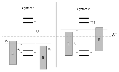
Figure 10: Schematic representation of two dual systems in the electron picture. The dotted line represents the particle-hole symmetric point $E^{*}$. Each system is equal to the mirror symmetry of its dual counterpart around $E^{*}$ in energy space . The electrons in System 1 must behave exactly the same as the holes in System 2, and reversely.  

This symmetry is slightly broken by our approximation scheme; the worst case is in the $\mathcal{N}=1$ CB regime. The reason could be due to the fact that at order $t_{\sigma}^{4}$ we do not treat the particle and hole contributions on an equal footing. Therefore, because the transition rates of the self-energies $\widehat{\Sigma}_{2\sigma}$ and $\widehat{\Sigma}_{3\sigma}$ have different values in the frequency range $\varepsilon_{\sigma}\leq\omega\leq\varepsilon_{\sigma}+U$, it leads to slightly asymmetric renormalization and broadening of the resonant peaks at $\varepsilon_{\sigma}$ and $\varepsilon_{\sigma}+U$, as can be shown in the particle-hole symmetric case, which affects the occupation number. For instance, at the particle-hole symmetric point ($\varepsilon_{\sigma}=-U/2$, $\mu_{L}=-\mu_{R}$), the dot occupation number $\langle n_{\sigma}\rangle$ is expected to be exactly $1/2$ in equilibrium or in the symmetric bias setting. Our numerical result shows deviation by a few percents at worst. However, it has almost no effect on the low-frequency density of states structure.

In order to restore the symmetry, one compute the Green function in the dual system. Because of the definition of the duality, we have the identity

$$\mathcal{G}^{\text{Syst1}}_{\sigma}(\omega)=\mathcal{C}\left[(\mathcal{G}^{\text{Syst2}}_{\sigma}(\omega)\right],$$ (E.3)

where Systems 1 and 2 are dual of each other. Using charge conjugation symmetry (cf.Appendix III) on System 2, we can express this equality in terms of electron Green functions only, that is

$$\mathcal{G}^{\text{Syst1}}_{\sigma}(\omega)=-\left[\mathcal{G}^{\text{Syst2}}_{\sigma}(-\omega)\right]^{*}.$$

As mentioned earlier, this equality is slightly violated at high frequencies by our approximation scheme. We therefore symmetrise the two by setting

$$\mathcal{G}^{r}_{\sigma}(\omega)=\left\{\mathcal{G}^{\text{Syst1}}_{\sigma}(\omega)-\left[\mathcal{G}^{\text{Syst2}}_{\sigma}(-\omega)\right]^{*}\right\}/2.$$ (E.4)

References

• (1) D. Goldhaber-Gordon, H. Shtrikman, D. Mahalu, D. Abusch-Magder, U. Meirav, and M. Kastner, Nature 391, 156 (1998); S.M. Cronenwett, T.H. Oosterkamp, and L.P. Kouwenhoven, Science 281,540 (1998); J. Schmid, J. Weis, K. Eberl, K. v. Klitzing, Physica B 256-258, 182 (1998); W. van der Wiel, S. de Franceschi, T. Fujisawa, J. Elzerman, S. Tarucha, and L.P. Kouwenhoven, Science 289, 2105 (2000).
• (2) J. Nygård, D.H. Cobden, and P.E. Lindelof, Nature (London) 408, 342 (2000).
• (3) P. W. Anderson, Phys. Rev. 124, 41 (1961).
• (4) L. Glazman and M. Raikh, Pis ma Zh. Eksp. Teor. Fiz. 8, 378 (1988) [JETP Lett. 47, 452 (1988)].
• (5) T.K. Ng and P.A. Lee, Phys. Rev. Lett. 61, 1768 (1988).
• (6) A.P. Hewson, The Kondo Problem to Heavy Fermions (Cambridge Univ. Press, Cambridge, 1993).
• (7) A. Kaminski, Y.V. Nazarov, and L.I. Glazman Phys. Rev. B 62, 8154 (2000).
• (8) P. Coleman, C. Hooley, and O. Parcollet, Phys. Rev. Lett. 86 4088 (2001).
• (9) O. Parcollet and C. Hooley, Phys. Rev. B 66, 085315 (2002).
• (10) A. Rosch, J. Kroha, and P. Wölfle, Phys. Rev. Lett. 87 156802 (2001).
• (11) A. Rosch, J. Paaske, J. Kroha, and P. Wölfle, Phys. Rev. Lett. 90, 076804 (2003).
• (12) J. Paaske, A. Rosch, J. Kroha, and P. Wölfle, Phys. Rev. B. 70, 155301 (2004).
• (13) R. Aguado and D.C. Langreth, Phys. Rev. Lett. 85, 1946 (2000).
• (14) N.S. Wingreen and Y. Meir, Phys. Rev. B 49, 11040 (1994).
• (15) R.C. Monreal and F. Flores, Phys. Rev. B 72, 195105 (2005).
• (16) R. Świrkowicz, J. Barnaś, and M. Wilczynśki, Phys. Rev. B 68, 195318 (2003).
• (17) A. Schiller and S. Hershfield, Phys. Rev. B 51, 12896 (1995).
• (18) R.M. Konik, H. Saleur, and A.W.W. Ludwig, Phys. Rev. Lett. 87, 236801 (2001);
• (19) R.M. Konik, H. Saleur, and A.W.W. Ludwig, Phys. Rev. B. 66, 125304 (2002) ; see also P. Mehta and N. Andrei, Phys. Rev. Lett. 96, 216802 (2006) in the case of an interacting spinless quantum dot.
• (20) R. Bulla, T.A. Costi, and T. Pruschke, Rev. Mod. Phys. 80, 395 (2008).
• (21) F. B. Anders, Phys. Rev. Lett. 101, 066804 (2008).
• (22) J.E. Han and R.J. Heary, Phys. Rev. Lett. 99, 236808 (2007).
• (23) D. Zubarev, Sov. Phys. Usp. 3, 320 (1960).
• (24) Lowell Dworin, Phys. Rev. 164, 818 (1967); 164, 841 (1967).
• (25) J. A. Appelbaum and D. R. Penn, Phys. Rev. 188, 874 (1969); Phys. Rev. B 3, 942 (1971).
• (26) C. Lacroix, J. Phys. F. 11, 2389 (1981).
• (27) Theumann, Phys. Rev. 178, 978 (1969); H. Mamada and F. Takano, Prog. Theor. Phys. 43, 1458 (1970); G. S. Poo, Phys. Rev. B 11, 4606 (1975); C. Lacroix, J. Appl. Phys. 53, 2131 (1982).
• (28) V. Kashcheyevs, A. Aharony, and O. Entin-Wohlman, Phys. Rev. B 73, 125338 (2006).
• (29) Y. Meir, N.S. Wingreen, and P. A. Lee, Phys. Rev. Lett. 70, 2601 (1993).
• (30) H.G. Luo, Z.J. Ying, and S.J. Wang, Phys. Rev. B 59, 9710 (1999).
• (31) J.E. Han, arXiv:0906.5577v1 (2009).
• (32) Y. Meir, N.S. Wingreen, Phys. Rev. Lett. 68, 2512 (1992).
• (33) F. D. M. Haldane, Phys. Rev. Lett. 40, 416 (1978).
• (34) J. Martinek, Y. Utsumi, H. Imamura, J. Barnaś, S. Maekawa, J. König, and G. Schön, Phys. Rev. Lett. 91, 127203 (2003); J. Martinek, M. Sindel, L. Borda, J. Barnaś, J. König, G. Schön, and J. von Delft, Phys. Rev. Lett. 91, 247202 (2003); J. Martinek, M. Sindel, L. Borda, J. Barnaś, R. Bulla, J. König, G. Schön, S. Maekawa and J. von Delft, Phys. Rev. B 72, 121302(R) (2005).
• (35) Y. Utsumi, J. Martinek, G. Schön, H. Imamura, S. Maekawa, Phys. Rev. B 71, 245116 (2005).
• (36) T.-K. Ng, Phys. Rev. Lett. 76, 487 (1996).
• (37) T.A. Costi, A.C. Hewson, Physica B, 163, 179 (1990).
• (38) Y. Meir, N.S. Wingreen, and P. A. Lee, Phys. Rev. Lett. 66, 3048 (1991).
• (39) O. Entin-Wohlman, A. Aharony, and Y. Meir, Phys. Rev. B 71, 035333 (2005).
• (40) See, for example, David C. Langreth and John W. Wilkins, Phys. Rev. B 6, 3189 (1972).
• (41) M. Grobis, I.G. Rau, R.M. Potok, H. Shtrikman, and D. Goldhaber-Gordon, Phys. Rev. Lett. 100, 246601 (2008).
• (42) S. De Franceschi, R. Hanson, W.G. van der Wiel, J.M. Elzerman, J.J. Wijpkema, T. Fujisawa, S. Tarucha, and L.P. Kouwenhoven, Phys. Rev. Lett. 89, 156801 (2002).
• (43) A. Kaminski, Yu. V. Nazarov, and L.I. Glazman, Phys. Rev. Lett. 83 384 (1999); Phys. Rev. B 62, 8154 (2000).
• (44) J. Paaske, A. Rosch, P. Wölfle, N. Mason, C. M. Marcus and J. Nygård, Nature Physics 2, 460-464 (2006).
• (45) E. C. Goldberg, F. Flores, and R. C. Monreal, Phys. Rev. B 71, 035112 (2005); Shiue-yuan Shiau, Sucismita Chutia, and Robert Joynt, Phys. Rev. B 75, 195345 (2007); Kicheon Kang and B. I. Min, Phys. Rev. B 52, 10689 (1995).
• (46) T.A. Costi, J. Kroha, and P. Wölfle, Phys. Rev. B 53, 1850 (1996).