Lifetime of double occupancies in the Fermi-Hubbard model

Abstract

We investigate the decay of artificially created double occupancies in a repulsive Fermi-Hubbard system in the strongly interacting limit using diagrammatic many-body theory and experiments with ultracold Fermions on optical lattices. The lifetime of the doublons is found to scale exponentially with the ratio of the on-site repulsion to the bandwidth. We show that the dominant decay process in presence of background holes is the excitation of a large number of particle hole pairs to absorb the energy of the doublon. We also show that the strongly interacting nature of the background state is crucial in obtaining the correct estimate of the doublon lifetime in these systems. The theoretical estimates and the experimental data are in fair quantitative agreement.

The non-equilibrium dynamics of a strongly interacting quantum many-body system is one of the most complex problems of modern physics. It encompasses various fields from the cosmology of the early universe cosmology or non-equilibrium jet production in high energy heavy ion collisions rhicjet to pump-probe experiments and operation of solid state devices under strong drive pump:probe in condensed matter physics. There are many open questions concerning non-equilibrium processes from both a theoretical and an experimental perspective, especially in the realm of condensed matter physics.

The theoretical understanding of interacting quantum many body systems in thermal equilibrium is on a much stronger footing, although strongly interacting systems like high temperature superconductors are not yet completely understood. This understanding is based on paradigms such as the quasiparticle excitations in the Fermi liquid model and ground states with broken symmetry described in terms of order-parameters and their fluctuations. The crucial point in all these paradigms is the hierarchy of energy scales of the quantum states. By working with a restricted set of states, organized according to their energy, it is possible to obtain a simplified model of the system. These low energy descriptions can capture the response of the system under small perturbations from equilibrium. However, in systems far from equilibrium, there is no organizing principle as the dynamics couples disparate states with widely different energies and linear response theory breaks down. This makes it hard to construct generic paradigms and one needs to solve the full microscopic Hamiltonian dynamics of an interacting quantum many-body system.

Some progress has been made for 1D systems, where it is often possible to obtain exact solutions for the eigenstates of the Hamiltonian. The absence of thermalization in 1D Bose systems has been predicted bg:notherm ; Olshanii2008 and observed bg:notherm:expt in cold atomic gases. However, these studies are hard to generalize to higher dimensions.

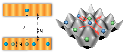
Figure 1: Stability of highly excited states in the single-band Hubbard model. Doubly occupied lattice sites are protected against decay by the on-site interaction energy $U$. The average kinetic energy of a single particle in a periodic potential is half the bandwidth $6J$. Thus the relaxation of excitations requires several scattering partners to maintain energy conservation.

In this context, it is useful to seek answers to concrete and focused questions involving non-equilibrium dynamics of specific strongly interacting systems. They have practical importance and help us gain better understanding of classes of non-equilibrium processes. Recent advances in controlling ultracold atomic gases with and without optical lattices have led to their emergence as perfect systems to study such phenomena. These systems, which can simulate strongly interacting model Hamiltonians, are essentially decoupled from external heat baths and hence the intrinsic non-equilibrium dynamics of the system can be studied easily. Compared to condensed matter systems, the low density in these systems results in long timescales for dynamics. As a result the system can be followed in real time without the use of ultrafast probes. Further, it is relatively easy to create and characterize an initial state far from the ground state, which is crucial since the dynamics depends heavily on the initial state.

In fact, questions of non-equilibrium dynamics and thermalization timescales are particularly important for these artificially engineered strongly correlated systems. Their key feature is the precise tunability of the Hamiltonian parameters which has made these systems ideal for the simulation of strongly interacting many-body Hamiltonians relevant to condensed matter systems. However, an implicit assumption in this comparison is that the system is in thermal equilibrium at low temperatures. In this context it is important to estimate the thermalization timescales as these systems are always characterized by a finite sample lifetime. Besides, several proposed methods to prepare the system in novel phases explicitly depend on adiabatic tuning of Hamiltonian parameters, which place stronger constraints on the possible sweep rates than mere demand of thermalization.

An important class of non-equilibrium problems is the decay of a high energy excitation into low energy excitations. This problem occurs in diverse contexts like multi-phonon decay of excitons in semiconductors multi:phonon , pump and probe experiments pump:probe and dynamics of nuclear resonances nuclear:resonance . In this paper, we study this problem in the non-equilibrium dynamics of artificially created double occupancies in the Fermi Hubbard Model in the strongly interacting regime. Specifically, we will look at the mechanism of doublon decay in this system and the relation of the doublon lifetime to the repulsive interaction. We study this dynamics both experimentally using ultracold Fermions on an optical lattice short:paper and theoretically using a projected Fermion model and diagrammatic resummations.

The doublon lifetime has practical implications for the sweep rates of Hamiltonian parameters in cold atom systems in the following way: The usual access to the strongly interacting regime is to start with a weakly interacting system and increase the ratio of interaction $U$ to the hopping energy $J$. As this ratio increases, the density of doublons in the system in equilibrium should decrease. Thus the doublon lifetime provides the dominant equilibration timescale for the system. We note here that this problem has structural similarities with the decay of a deeply bound excitonic state through multi-phonon processes in semi-conductors multi:phonon , but as we shall see, the strong Hubbard repulsion modifies the situation in an essential way.

Our main results are (i) The decay of a doublon is a slow process as the doublon needs to distribute a large energy ($\sim U$) to other excitations in the system which have a much smaller energy scale. (ii) The primary mode of decay of the doublon involves creation of particle-hole pairs in the background system. (iii) The decay rate scales as $\Gamma\sim C\,J\exp(-\alpha\,U/J)$ and the decay becomes slower with increasing interaction. We obtain $C$ and $\alpha$ from experiments and from theoretical calculation. (iv) We find that the interactions between pairs of single Fermions, which in our model are induced by projection, are important and quantitatively affect the timescale of the decay. Thus the strongly correlated character of the system changes the dynamics in an essential way.

The paper is organized as follows: In Section I we discuss the various possible decay mechanisms of the doublon in these systems and give a scaling argument for the decay rate in each case. In Section II we describe the experiments and its results. In Section III we discuss the most relevant decay mechanism in our experiments and develop the theoretical model for doublon decay. In Section IV we outline the diagrammatic method to compute the doublon lifetime. In Section V we discuss the theoretical results and its comparison with the experiments. We conclude in section VI by discussing the importance of these results and future directions. The technical details of the theory are described in relevant appendices.

I Decay mechanisms for a doublon

The single-band Hubbard model describing the Fermions on an optical lattice is given by Jaksch1998

$$H=-J\sum_{\langle ij\rangle\sigma}c^{\dagger}_{i\sigma}c_{j\sigma}+U\sum_{i}n_{i\uparrow}n_{i\downarrow}.$$ (1)

At large $U/J$, this model has three main energy scales. There is the energy of double occupancies, given by the Hubbard repulsion $U$, the kinetic energy of the Fermions given by the tunneling $J$ and the superexchange scale $J_{ex}=4J^{2}/U$, which governs the spin dynamics in the system. At large $U/J$, these scales are well separated from each other, $U\gg J\gg J_{ex}$. As we show below, the separation of the energy scale $U$ from the other energy scales $J$ and $J_{ex}$ leads to a slow decay of doublons in the system.

In order to decay the doublon has to give up its energy $\sim U$ to other excitations in the system. Let the typical energy of a possible excitation be $\epsilon_{0}$ where $\epsilon_{0}$ can be either $\sim J$ or $\sim J_{ex}$ depending on the background state in which the doublon is propagating. We assume that $\epsilon_{0}\ll U$, so that a large number $n\sim U/\epsilon_{0}$ of excitations must be created to satisfy energy constraints. The matrix element for this process can be calculated by an $n^{th}$ order perturbation theory and is given by

$$M\sim\frac{J}{\epsilon_{0}}\times\frac{J}{2\times\epsilon_{0}}\times\dots\times\frac{J}{n\times\epsilon_{0}}.$$ (2)

The decay rate is $\sim M^{2}$ in units of $J$. Using Stirling’s formula, and the fact that $n\epsilon_{0}=U$, we find that for large $n$ the decay rate scales as

$$\Gamma\sim J(J/U)^{\frac{U}{\epsilon_{0}}}\sim CJ\exp(-\alpha\,U/\epsilon_{0}\,\log(U/J))$$ (3)

where $C$ and $\alpha$ are constants which we will extract from detailed calculations and experimental data.

In order to discuss the specific decay mechanisms of a doublon, we need to specify the state of the background system in which the doublon is propagating. If the system is a homogeneous Mott insulator at half-filling, the only possible candidate for transfer of energies are spin excitations with bandwidth $\epsilon_{0}\sim J_{ex}$. This leads to the decay rate scaling as $\Gamma\sim J\exp(-\alpha\,U^{2}/J^{2}\log(U/J))$ and is an extremely slow process. However, if the system is compressible, the dominant energy transfers are to kinetic energy of the Fermions through creation of particle-hole pairs with typical energy $\epsilon_{0}\sim J$. This leads to the decay rate scaling as $\Gamma\sim J\exp(-\alpha\,U/J\log(U/J))$. This is a much faster decay process and will dominate over decay through spin excitations. We note that compressible states with holes can exist (i) at the edges of systems with confining traps or (ii) in the bulk of the system as a result of a large density of doublons created by modulation spectroscopy. In a trapped system, there is another possibility of giving up the energy to the potential energy of the Fermions at the edges. This however involves transfer of particles from the center to the edges of the trap and is usually a much slower process for typical shallow traps used in cold atom experiments.

As we will see in the next section our experimental system has a lot of holes and we can eliminate many of the possible decay mechanisms for our experimental configuration. Therefore, in this Paper we shall focus on the dominant doublon decay channel involving excitation of particle hole pairs.

II Experiments

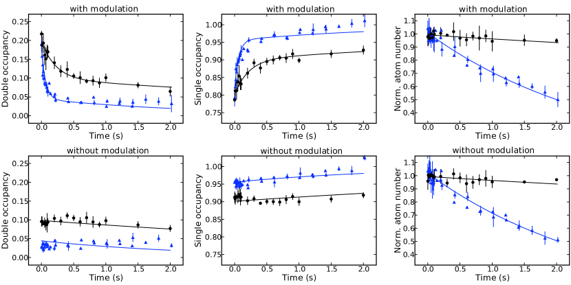
Figure 2: Time evolution of double occupancy, single occupancy and total atom number for different ratios $U/6J$. In the upper row, the system was previously excited via lattice modulation. The bottom row shows the reference measurement for the determination of the residual dynamics. The round data points were recorded using a $m_{F}=\left(-9/2,-7/2\right)$ spin mixture with $U/h=1.4\,\text{kHz}$ and $J/h=70\,\text{Hz}$, whereas the triangular data points show a $\left(-9/2,-5/2\right)$ mixture with $U/h=3.2\,\text{kHz}$ and $J/h=100\,\text{Hz}$. The solid lines are simultaneous fits of the integrated population equations of Eq. II. The total atom numbers are scaled to the initial values. Single occupancy and double occupancy are the fraction of atoms residing on sites of the respective type. Due to different detection efficiencies for hyperfine states the sum of double and single occupancy can be higher than one. Error bars denote the statistical error of at least four identical measurements.

This section describes the experimental steps towards the observation of doublon relaxation: Initially, a sample of repulsively interacting, ultracold fermions is produced and loaded into an optical lattice. Starting from this equilibrium state, we create additional double occupancies via lattice modulation. Immediately after this excitation we measure the time evolution of the double occupancy. We remove the influence of inelastic loss processes by comparing to a reference measurement and extract the elastic doublon lifetime using a simple rate equations model. Finally, this elastic lifetime is normalized with the tunneling time $J/h$ and found to depend exponentially on $U/6J$.

The experimental sequence used to produce quantum degenerate Fermi gases has been described in detail in previous work Jordens2008 . In brief, we prepare $(50\pm 5)\times 10^{3}$ ⁴⁰K atoms at temperatures below $15\%$ of the Fermi temperature $T_{\mathrm{F}}$ in a balanced mixture of two magnetic sublevels of the $F=9/2$ hyperfine manifold. The confinement is given by a crossed beam dipole trap with trapping frequencies $\omega_{x,y,z}=2\pi\times(35,23,120)\,\text{Hz}$. To access a wide range of repulsive interactions we make use of two magnetic Feshbach resonances. With a $m_{F}=\left(-9/2,-7/2\right)$ spin mixture, we realize scattering lengths of $98\,a_{0}$ and $131\,a_{0}$, where $a_{0}$ is the Bohr radius Regal2003 . The $\left(-9/2,-5/2\right)$ spin mixture allows us to reach the strongly repulsive regime with scattering lengths of $374\,a_{0}$, $571\,a_{0}$ and $672\,a_{0}$ newResonance . After adjusting the scattering length to the desired value, we add a three-dimensional optical lattice of simple cubic symmetry. The lattice depth is increased in $200\,\text{ms}$ to final values between $6.5E_{R}$ and $12.5E_{R}$ in units of the recoil energy $E_{R}=h^{2}/2m\lambda^{2}$. Here $h$ is Planck’s constant, $m$ the atomic mass and $\lambda=1064\,\text{nm}$ the wavelength of the lattice beams. The lattice beams have Gaussian profiles with $1/e^{2}$ radii of $w_{x,y,z}=(160,180,160)\,\mu\text{m}$ at the position of the atoms. For a given scattering length and lattice depth, $J$ and $U$ are inferred from Wannier functions Jordens2008 ; Jaksch1998 . Their statistical and systematic errors are dominated by the lattice calibration and the accuracies in width and position of the two Feshbach resonances Regal2003 ; newResonance .

Depending on $U$ and $J$ the final states of the system range from metallic to Mott insulating phases, but always with a double occupancy below $15\%$. This equilibrium system is now excited by a sinusoidal modulation of the lattice depth with a frequency close to $U/h$. This causes an increase of the double occupancy between 5 and $20\%$ as compared to the initial state. The modulation amplitude is $10\%$ on all three axes, while the modulation duration was chosen such that the amount of doubly occupied lattice sites saturates Kollath2006 ; Hassler2008 ; Jordens2008 ; Huber2008 ; Sensarma2009 . The system is now in a highly excited non-equilibrium state with double occupancies between 15 and $35\%$.

After free evolution at the initial lattice depth and interaction strength for a variable hold time up to $4$ s we probe the remaining double occupancy of the system. This is accomplished by a sudden increase of the lattice depth to $30\,E_{\mathrm{R}}$, which prevents further tunneling. We then measure the amount of atoms residing on singly (doubly) occupied sites $N_{\mathrm{s}}$ ($N_{\mathrm{d}}$) by encoding the double occupancy into a previously unpopulated spin state using radio frequency spectroscopy Jordens2008 . Combining Stern-Gerlach separation and absorption imaging we obtain the single occupancy $n_{\mathrm{s}}=N_{\mathrm{s}}/N_{\mathrm{tot}}$, double occupancy $n_{\mathrm{d}}=N_{\mathrm{d}}/N_{\mathrm{tot}}$ and total atom number $N_{\mathrm{tot}}=N_{\mathrm{s}}+N_{\mathrm{d}}$.

The time evolution of the double and single occupancy and of the total atom number is shown for two different parameter sets in the upper row of Fig. 2. In both cases, the double occupancy decays exponentially within the observation time, and the single occupancy rises accordingly. The time evolution of the total atom number, however, exhibits a remarkable difference between the $\left(m_{\mathrm{F}}=-9/2,-7/2\right)$ and the $\left(m_{\mathrm{F}}=-9/2,-5/2\right)$ spin mixture: Whilst the atom number of the $\left(-9/2,-7/2\right)$ sample remains rather constant, the $\left(-9/2,-5/2\right)$ sample suffers from an atom number reduction of 50 $\%$ within $2$ s. This behavior can be observed for all parameter sets and is a consequence of the shorter lifetime of a $\left(-9/2,-5/2\right)$ spin mixture.

The only relevant process described by the Fermi-Hubbard model is the decay of a doublon into two single particles which remain within the system. The time associated with this process will be called doublon lifetime. In an experiment, inelastic processes may occur, resulting in atoms exiting the system. For a valid comparison with theory it is therefore crucial that these processes do not interfere with the determination of the doublon lifetime. In the following, we show how we eliminate the influence of inelastic loss processes on the observation of the doublon decay.

For every dataset on doublon decay after lattice modulation, we record a corresponding reference dataset without lattice modulation, but with the same system parameters. Two of these reference datasets are presented in the bottom row of Fig. 2. They show the dynamics of double occupancies and atom number governed by inelastic processes, which are not taken into account by the Fermi-Hubbard model.

Combining these two measurements, we can unambiguously extract the doublon lifetime by simultaneously fitting a system of coupled rate equations. They describe the population dynamics in the optical lattice, considering three general processes:

$$\Delta\dot{N}_{\mathrm{d}} = -\left(\frac{1}{\tau_{\mathrm{D}}}+\frac{1}{\tau_{\mathrm{in}}}+\frac{1}{\tau_{\mathrm{loss}}}\right)\Delta N_{\mathrm{d}}$$

$$\dot{N}_{\mathrm{d},0} = -\left(\frac{1}{\tau_{\mathrm{in}}}+\frac{1}{\tau_{\mathrm{loss}}}\right)N_{\mathrm{d},0}$$ (4)

$$\dot{N}_{\mathrm{s}} = \frac{1}{\tau_{\mathrm{D}}}\Delta N_{\mathrm{d}}-\frac{1}{\tau_{\mathrm{loss}}}N_{\mathrm{s}}$$

The total number of atoms on doubly occupied sites $N_{\mathrm{d}}$ is written as the sum of the equilibrium population $N_{\mathrm{d},0}$ and the additional amount of double occupancy $\Delta N_{\mathrm{d}}$ created by the lattice modulation. The three time constants correspond to three independent local decay processes differing in the type of site they affect: $\tau_{\mathrm{D}}$ describes the population flow from doubly occupied to singly occupied lattice sites visible as a decay of double occupancy within $0.01-1\,\text{s}$ that is accompanied by a rise of the single occupancy. We identify this time with the lifetime of doublons. The other two times denote loss time constants, which lead to a reduction of the total atom number: $\tau_{\mathrm{loss}}$ corresponds to losses affecting both site types in the same manner, which is only observed in the total atom number. Additional inelastic losses on doubly occupied sites are summarized by $\tau_{\mathrm{in}}$, visible as a simultaneous decay of both the total atom number and double occupancy. This model does not account for changes of the decay times during the decay or for higher order terms in the rate equations.

Since the modulation has no influence on the evolution of the total atom number, this procedure removes the influence of $\tau_{\text{in}}$ and $\tau_{\text{loss}}$. A reliable determination of the doublon lifetime $\tau_{\text{D}}$ is thus possible if it differs significantly from the loss times. The model and the observation are found to agree very well within experimental uncertainties, as can be seen in Fig. 2.

We measure this doublon lifetime for various tunneling and interaction strengths, covering a parameter range where $J$ and $U$ each differ by at least a factor of four. The determined lifetimes vary over two orders of magnitude, as shown in Fig. 3. Furthermore, the lifetime clearly does not depend on the tunneling energy or the interaction energy alone.

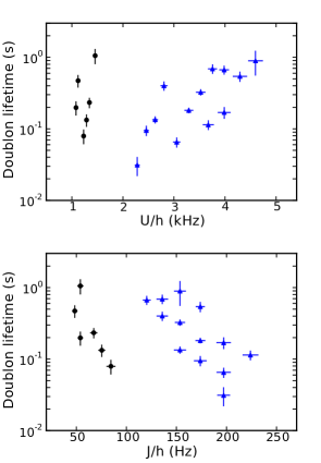
Figure 3: Doublon lifetime as a function of $U$ and $J$. The round data points show the fit results to datasets as shown in Fig . 2, obtained with a $\left(-9/2,-7/2\right)$ spin mixture while the triangular points correspond to the $\left(-9/2,-5/2\right)$ mixture. Error bars denote the confidence intervals of the lifetime fits and the statistical errors in $U$ and $J$.

Since the tunneling time $h/J$ is the dominant timescale of dynamics in an optical lattice, it appears natural to express the doublon lifetime in units of $h/J$. After this rescaling, we found that, to a good extent, the doublon lifetime only depends on the ratio $U/6J$.

Fig. 4 shows the doublon lifetime in units of the tunneling time versus $U/6J$ on a logarithmic scale. Remarkably, over the entire parameter range the data collapses in a corridor and can be described by an exponential function of the form:

$$\frac{\tau_{D}}{h/J}=C\,\exp\left(\alpha\frac{U}{6J}\right).$$ (5)

The scaling exponent $\alpha$ is found to be $\alpha=0.82\pm 0.08$ with $C=1.6\pm 0.9$. This is in reasonable quantitative agreement with the following calculation of the doublon lifetime.

The slight offset between the two spin mixtures in Fig. 4 could be due to the fact that the absolute values for $U$ and $J$ differ significantly between the $\left(-9/2,-5/2\right)$ and the $\left(-9/2,-7/2\right)$ mixture offsetalpha . Whilst the ratio between interaction energy and kinetic energy $U/6J$, which dominates the dynamics, lies in the same range, the absolute values also matter in an inhomogeneous system. For the $\left(-9/2,-7/2\right)$ mixture the higher ratio of chemical potential to on-site interaction is expected to lead to a higher filling in the trap centre and consequently to a higher equilibrium double occupancy $N_{d,0}$ than for the $\left(-9/2,-5/2\right)$ mixture. It is conceivable that this difference modifies the dynamics of doublon creation and doublon relaxation.

In additional measurements we examined the dependence of the doublon lifetime on the initial double occupancy $\Delta N_{d}$ and on the total atom number $N$. In the former case, we reduced the lattice modulation amplitude from 10% to 5%, resulting in $\Delta N_{d}=9\%$ instead of $\Delta N_{d}=18\%$, while keeping all other parameters constant with $U/6J=4.5$. The measured lifetimes agree within the error bars, they are $\tau_{\mathrm{D},5\%}=(77\pm 25)\times h/J$ and $\tau_{\mathrm{D},10\%}=(58\pm 10)\times h/J$, respectively. In the latter case, we prepared two otherwise identical samples at $U/6J=3.4$ with $N=(49\pm 7)\times 10^{3}$ atoms and with $N=(26\pm 4)\times 10^{3}$ atoms, respectively, yielding $\tau_{\mathrm{D},49000}=(11\pm 2)\times h/J$ and $\tau_{\mathrm{D},26000}=(19\pm 2)\times h/J$.

This shows that, although there is a dependence on the total density and on the doublon density, these effects are small compared to the dominant scaling with $U/6J$. Their systematic study is beyond the scope of this work.

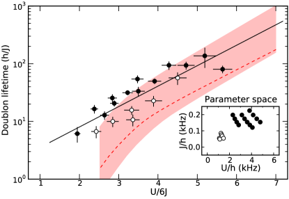
Figure 4: Semilogarithmic plot of doublon lifetime $\tau_{D}$ vs. $U/6J$. The lifetime is extracted from datasets as shown in Fig. 2. Solid and hollow circles denote the $\left(-9/2,-5/2\right)$ and $\left(-9/2,-7/2\right)$ spin mixture respectively, while the dashed line shows the theoretical result at half filling. The solid line is a fit of Eq. 5 to the experimental data, yielding $\alpha=0.82\pm 0.08$, whereas for the theory curve the asymptotic slope at large $U/6J$ is $\alpha_{T}=0.80$. The shaded corridor was obtained by varying the filling factor in the calculation by $0.3$. This has only a weak effect on the slope. The inset shows the parameters used to realize the different values of $U/6J$. Error bars denote the confidence intervals of the lifetime fits and the statistical errors in $U/6J$. The systematic errors in $U/6J$ and $\tau_{D}=h/J$ are estimated to be 30% and 25%, respectively.

III Theoretical Model of Doublon Decay

We consider the decay of an isolated doublon moving in the homogeneous background of a compressible state of single Fermions. Before constructing a model for doublon decay, we focus on the dominant mechanism of decay. In the experiments, lattice modulation created $15-35\%$ double occupancies. Assuming an initial half-filled system, half the amount of holes were also created in the system. At these hole densities, the kinetic energy assisted decay scaling as $\sim\exp(-U/J)$ is much faster than the spin fluctuation or doublon-doublon collision assisted decay which scale as $\sim\exp(-U^{2}/J^{2})$ Mott:decay . Further, the population of higher bands can be excluded, since $U$ is always smaller than half the band gap. We also note that as the difference between $U$ and the chemical potential is always positive, confinement assisted decay of doublons near the edge of the cloud is unlikely, as the accessible confinement energy is not very large, and the tunneling rate is very small. Finally, a homogeneous compressible background is justified since most of the doublons are created in the central region of the trap, where the filling is highest, and decay at most within a few sites of where they are produced The estimated travel distance for a random walk during the decay process is not more than $\sqrt{\tau_{\mathrm{D}}J/h}\lesssim 10$ sites, which is less than the cloud radius.

In our experiments, the doublons and holes are created at finite density by driving the system with optical lattice modulations. The relaxation of the system to equilibrium involves two very different time scales. The first timescale is associated with the relaxation of holes and doublons to a state of quasi-equilibrium without the decay of doublons. The second timescale, which is the focus of this paper, is associated with the decay of doublons into singles. We expect that the second timescale is much slower than the first. Moreover, we expect that non-linear effects of doublon decay as doublon-doublon scattering can be neglected since their kinetic energy $\sim J^{2}/U$ is small. Thus in this paper we consider the problem of the decay of a single doublon in the background of equilibrated Fermions.

To construct our model Hamiltonian, we explicitly treat the doublon as a separate entity from the background Fermions. This approximation is justified in the strongly interacting limit due to the separation of doublon and background Fermion time-scales. We split the complete Hamiltonian of the system into three parts

$$H=H_{f}+H_{d}+H_{fd},$$ (6)

where $H_{f}$ describes the background Fermion subsystem—which we model as the projected Fermi sea, $H_{d}$ describes the on-site interaction of the pair of Fermions that make up a doublon, and $H_{fd}$ describes the Fermion-doublon interaction. The details of how to separate the Fermi-Hubbard Hamiltonian into the above three parts via projection operators are discussed in Appendix  A. The projection operators induce interactions in the Fermion subsystem as well as between the Fermions and the doublons. The Fermion doublon interactions are responsible for the doublon decay, and the Fermion-Fermion interactions modify the lifetime substantially.

As mentioned above, we expect hole density in these systems to be $\sim 15\%$. At such high hole densities the projected Fermi sea is a good approximation for the background state. Further the temperature of the system is high enough ($T\sim J$) to prevent formation of more ordered states like superfluids.

Except for the single doublon that is undergoing decay, the large energy cost of double occupancies is taken into account by projecting out configurations with double occupancies from a simple Fermi sea. In the projected subspace, the Fermions can only hop in the presence of empty sites (holes) and are governed by the effective Hamiltonian

$$H_{f}=-J\sum_{\langle ij\rangle,\sigma}(1-n_{i\overline{\sigma}})c^{\dagger}_{i\sigma}c^{\phantom{\dagger}}_{j\sigma}(1-n_{j\overline{\sigma}})-\mu\sum_{i,\sigma}c^{\dagger}_{i\sigma}c^{\phantom{\dagger}}_{i\sigma}$$ (7)

where $c^{\dagger}_{i\sigma}$ creates a Fermion with spin $\sigma$, $n_{i\sigma}$ is the corresponding number operator, and $\mu$ is the chemical potential. Expanding out the Hamiltonian one gets $H_{f}=H_{f}^{0}+H_{p}$, with

$$H_{f}^{0} = -J\sum_{\langle ij\rangle,\sigma}c^{\dagger}_{i\sigma}c^{\phantom{\dagger}}_{j\sigma}-\mu\sum_{i,\sigma}c^{\dagger}_{i\sigma}c^{\phantom{\dagger}}_{i\sigma},$$ (8)

$$H_{p} = J_{1}\sum_{\langle ij\rangle,\sigma}n_{i\overline{\sigma}}c^{\dagger}_{i\sigma}c^{\phantom{\dagger}}_{j\sigma}+c^{\dagger}_{i\sigma}c^{\phantom{\dagger}}_{j\sigma}n_{j\overline{\sigma}},$$ (9)

where we have replaced $J$ by $J_{1}$ in the second term. $J_{1}$ will be treated as a perturbation parameter to organize the calculation but we will put $J_{1}=J$ at the end of the calculation. $H_{p}$, coming from the projection operators can thus be interpreted as a Fermion-Fermion scattering term which leads to the creation of particle-hole pairs. We thus see that projection induces interaction between the Fermions.

We note that the scattering is always between Fermions of opposite spins. Since we will be interested in calculating Feynman diagrams, we note that the interaction vertex for the Fermion Fermion scattering can be written as $J_{1}(\gamma_{\bf k}+\gamma_{{\bf k}-{\bf q}})$, where ${\bf k}$ and ${\bf k}-{\bf q}$ are momenta of the incoming and outgoing Fermion with the same spin and $\gamma_{\bf k}=2\sum_{i=1}^{D}\cos k_{i}$ in $D$ dimensions. This is depicted in first row of Table  1.

Throughout our treatment, we leave out terms such as $-J\,n_{i\overline{\sigma}}c^{\dagger}_{i\sigma}c^{\phantom{\dagger}}_{j\sigma}n_{j\overline{\sigma}}$ in Eq. (7) involving six or more fermion creation/annihilation operators. Intuitively such terms are rare because they involve collisions of multiple particles.

Interaction	Diagram	$\begin{array}[]{c}\text{Vertex}\\ \left[\begin{array}[]{c}\text{Momentum}\\ \text{Avg. Vertex}\end{array}\right]\end{array}$
Fermion-Fermion Scattering		$\begin{array}[]{c}J(\gamma_{{\bf k}_{1}}+\gamma_{{\bf k}_{2}})\\ \\ \left[J\sqrt{2z}\,\right]\end{array}$
Doublon-Fermion Scattering		$\begin{array}[]{c}J(\gamma_{{\bf p}-{\bf q}}+\gamma_{\bf p}+\gamma_{\bf q})\\ \\ \left[J\sqrt{z}\,\right]\end{array}$
Doublon Decay		$\begin{array}[]{c}J(\gamma_{{\bf k}}+\gamma_{{\bf p}-{\bf k}})\\ \\ \left[J\sqrt{2z}\,\right]\end{array}$

Table 1: Interaction vertices for different processes in the model for doublon decay. The single lines are Fermion propagators while the double lines are doublon propagators. The top entry in the right-most column is the corresponding vertex function, while the bottom entry is the “momentum averaged” vertex function that we use in the our resummation technique. The first row corresponds to $H_{p}$ (Eq. 9) while the next two rows correspond to the two terms that make up $H_{fd}$ (Eq. 11). Here $\gamma_{k}=2(\cos(k_{x})+\cos(k_{y})+\cos(k_{z}))$ and $z$ is the coordination number, $z=6$ for 3D cubic lattice.

We now consider the decay of a single doublon in this background state. The doublon ($d$) and Fermion-doublon ($fd$) Hamiltonians can be written as

$$H_{d} =U\sum_{i}d^{\dagger}_{i}d_{i},$$ (10)

$$H_{fd} =J\sum_{\langle ij\rangle\sigma}(d^{\dagger}_{i}d^{\phantom{\dagger}}_{i}+d^{\dagger}_{j}d^{\phantom{\dagger}}_{j}+d^{\dagger}_{j}d^{\phantom{\dagger}}_{i})c^{\dagger}_{i\sigma}c^{\phantom{\dagger}}_{j\sigma}$$ (11)

$$\quad\quad\quad\quad\quad+d_{i}\sigma c^{\dagger}_{i\sigma}c^{\dagger}_{j\overline{\sigma}}(1-n_{j\sigma})+\text{H.c.},$$

where H.c. stands for the Hermitian conjugate of the preceding term. The doublon interacts with the Fermions in two different ways: (i) it can scatter off a Fermion leading to the hopping of doublons with back-flow of Fermions; (ii) it can decay by creating a singlet particle-particle pair.

The interaction vertices of the doublon with the Fermions are given in second and third rows of Table  1. The vertex for scattering off particle-hole pairs is $J(\gamma_{{\bf p}-{\bf q}}+\gamma_{\bf q}+\gamma_{\bf k})$, where ${\bf p}$ is the momentum of the incoming doublon, ${\bf q}$ is the momentum of the outgoing Fermion and ${\bf k}$ the momentum of the outgoing hole. The corresponding vertex for decay through singlet creation is given by $J(\gamma_{\bf k}+\gamma_{{\bf p}-{\bf k}})$ where ${\bf k}$ and ${\bf p}-{\bf k}$ are the momenta of the Fermions created.

We assume that we are looking at the decay of a single doublon i.e. while the doublon is affected by the presence of the background Fermions, the Fermions are unaffected by the presence of the doublon. The motivation for this assumption is that the experimentally observed decay rate depends only weakly on the doublon density.

IV Diagrammatic Computation of Doublon Lifetime

Our strategy for finding the lifetime of a doublon is to calculate the doublon Green function

$${\cal G}_{d}(\omega)=[\omega-U-\Sigma_{d}(\omega)]^{-1},$$ (12)

where $\Sigma_{d}$ is the self-energy arising from interaction with Fermions. The imaginary part of the self-energy at $\omega=U$ then gives the decay rate $\Gamma$ and its inverse is the required lifetime $\tau$. Since we are interested in the high frequency response, the momentum dependence of the self energy should be negligible in this limit.

We perform the calculation at $T=0$, where the relation between imaginary part of the self-energy and decay rate is exact. At finite temperatures $\text{Im}~{}\Sigma(\omega)$ has an extra contribution due to scattering on particle-hole pairs created by thermal fluctuations. Thus, we must compute the scattering rate separately, and subtract it from $\text{Im}~{}\Sigma(\omega)$ to obtain the decay rate. However, since we are looking at frequencies $\sim U$, ignoring thermal fluctuations is justified for $T\ll U$, which is the regime of interest.

Physically, there are two important processes for the doublon decay. A doublon can lose its energy either by creating a large number of particle-hole pairs, each with an energy $\sim J$, or by creating a few high energy particle-hole pairs, each of which is unstable and creates a shower of particle hole pairs of low energies. The first process is a high order diagram in the doublon self-energy while the second process comes from high order diagrams in the Fermion self-energy. We find that combinations of both processes give important contributions to the doublon decay rate.

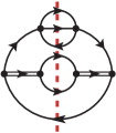
Figure 5: A Typical doublon self-energy diagram. The double lines are bare doublon propagators while the single lines are bare Fermion propagators. The dashed line cuts the diagram in half and shows the final products of the process represented by this diagram

The typical doublon self-energy diagram (Fig. 5) depicts a process of creation of a number of particle and hole excitations. Since we are interested in the imaginary part of the self energy at $\omega=U$, the Fermion lines crossing the dashed line which cuts the diagram in half should be on-shell and their energies must add up to $U$. The leading order contributions to the decay rate thus come from the diagrams which maximize the number of Fermions that cross the dashed line while minimizing the number of interaction vertices.

Our approach for obtaining the doublon self energy consists of (1) obtaining the projected Fermi sea Green function, and (2) using it to obtain the doublon self-energy. We make the dilute doublon approximation, and assume that the Fermion Green function is independent of the doublon Green function. We proceed by formulating a diagrammatic resummation technique for the doublon self-energy in the following subsection. In doing so, we relate the doublon self-energy to the Fermion Green function, which we calculate in the next two subsections.

IV.1 Doublon Self-Energy

For large $U/J$, doublon decays into a large number of particle-hole pairs, and therefore one needs to compute high order diagrams to obtain the doublon self-energy (for creation of $n$ pairs, one needs to compute $\sim 2n!$ diagrams). It is then much preferable to resum a class of diagrams, rather than evaluate an exponentially increasing number of them. We use a self-consistent non-crossing approximation to achieve this resummation. The propagator diagrams are shown in Fig. 6, where the doublon lines with squiggles represent the full doublon Green function to be obtained self-consistently and the thick single lines are the Fermion propagators.

At this point, we make an additional approximation, and replace the ${\bf k}$-dependent vertex functions $\Lambda_{\bf k}$ by momentum averaged vertex functions $\sqrt{\langle\Lambda_{\bf k}^{2}\rangle}$ listed in Table 1. The basis of this approximation, is that within our resummation scheme, the vertex functions always occur in pairs with identical and largely arbitrary momentum indices, as can be seen from the self-consistent equation represented in Fig. 6. The self-consistent equation, therefore, contains the product of this pair of vertex functions, and we replace this product by its momentum averaged value.

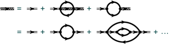
Figure 6: Self-consistency equation for the doublon propagator (top) and some typical diagrams that make up the full propagator (bottom). Thin double-lines indicate the bare doublon propagator, the double-lines with a squiggle the full (resummed) doublon propagator, and thick single-lines the full (resummed) Fermion propagator.

Having replaced the momentum-dependent vertex functions by momentum-independent ones, we can replace Green functions and self-energies by their momentum averaged counterparts. With this modification, the doublon self-energy is given by

$$\Sigma_{d}^{{}^{\prime\prime}}(\omega) \!=\!zJ^{2}C^{{}^{\prime\prime}}(\omega)\!-\!2zJ^{2}\int_{0}^{\omega}\frac{d\omega^{\prime}}{\pi}S^{{}^{\prime\prime}}(\omega^{\prime}){\cal G}_{d}^{{}^{\prime\prime}}(\omega\!-\!\omega^{\prime})$$ (13)

$$\Sigma_{d}^{{}^{\prime}}(\omega) \!=\!zJ^{2}C^{{}^{\prime}}(\omega)\!-\!2zJ^{2}\int_{-\infty}^{0}\frac{d\omega^{\prime}}{\pi}S^{{}^{\prime\prime}}(\omega^{\prime}){\cal G}_{d}^{{}^{\prime}}(\omega\!-\!\omega^{\prime})$$

$$\quad\quad\quad\quad+2zJ^{2}\int_{0}^{\infty}\frac{d\omega^{\prime}}{\pi}{\cal G}_{d}^{{}^{\prime\prime}}(\omega^{\prime})S^{{}^{\prime}}(\omega\!-\!\omega^{\prime})$$ (14)

where $\Sigma_{d}$, $C$, and $S$ are the retarded doublon self-energy, Fermionic particle-particle and particle-hole propagators respectively ftnote_1 , and the primes ^′ and ^′′ denote the real and imaginary parts, respectively. The particle-particle and particle-hole propagators are given by

$$S^{{}^{\prime\prime}}(\omega) \!=\!-\!\!\int_{0}^{\omega}\frac{d\omega^{\prime}}{\pi}{\cal G}_{f}^{{}^{\prime\prime}}(\omega^{\prime}){\cal G}_{f}^{{}^{\prime\prime}}(\omega^{\prime}\!-\!\omega)$$ (15)

$$S^{{}^{\prime}}(\omega) \!=\!-\!\!\int_{-\infty}^{0}\!\!\frac{d\omega^{\prime}}{\pi}{\cal G}_{f}^{{}^{\prime\prime}}(\omega^{\prime})[{\cal G}_{f}^{{}^{\prime}}(\omega^{\prime}\!-\!\omega)+{\cal G}_{f}^{{}^{\prime}}(\omega^{\prime}\!+\!\omega)]$$ (16)

$$C^{{}^{\prime\prime}}(\omega) \!=\!-\!\!\int_{0}^{\omega}\frac{d\omega^{\prime}}{\pi}{\cal G}_{f}^{{}^{\prime\prime}}(\omega^{\prime}){\cal G}_{f}^{{}^{\prime\prime}}(\omega-\omega^{\prime})$$ (17)

$$C^{{}^{\prime}}(\omega) \!=\int_{-\infty}^{0}\frac{d\omega^{\prime}}{\pi}{\cal G}_{f}^{{}^{\prime\prime}}(\omega^{\prime}){\cal G}_{f}^{{}^{\prime}}(\omega-\omega^{\prime})$$

$$\quad\quad\quad\quad-\int_{0}^{\infty}\frac{d\omega^{\prime}}{\pi}{\cal G}_{f}^{{}^{\prime\prime}}(\omega^{\prime}){\cal G}_{f}^{{}^{\prime}}(\omega^{\prime}+\omega)]$$ (18)

where ${\cal G}_{f}(\omega)=\sum_{\bf k}{\cal G}_{f}({\bf k}\omega)$ is the momentum averaged Fermion Green function and the primes ^′ and ^′′ denote the real and imaginary parts. These equations, together with the equation for the doublon Green function, Eq. (12), define a system of self-consistent equations for the doublon self-energy.

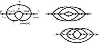
Figure 7: Typical diagrams for the doublon Green function that are not accounted for in the resummation procedure as they contain crossing Fermion lines. Here, double-lines stand for bare doublon propagators and thick single-lines the full (resummed) Fermion propagator. For reasons explained in the main text, these crossing diagrams do not contribute to the doublon decay, as the vertex factors are not paired and thus average to zero upon momentum integration. To see this, the momenta and a pair of vertices in the first, pretzel-like, diagram are labeled. Notice that the $\gamma$ vertex factors have different momentum labels, these would have been identical for the case of a non-crossed diagram.

In this section we have made two approximations: (1) we replaced the momentum dependent vertex functions by momentum independent ones, and (2) we have left out a large number of diagrams with crossing Fermion lines (see Fig. 7 for some typical examples). To verify these approximations, we have explicitly computed all diagrams up to $6^{th}$ order in a Fermi Golden Rule calculation, which is free of these approximations (see Appendix B for details). We find that the decay rate computed via Fermi Golden Rule matches very well with the resummation result. Further, within Fermi Golden Rule calculation we empirically verify that the contribution of crossed diagrams to the doublon self-energy is indeed negligible. Intuitively, the reason for this seems to be that the Fermion-doublon interaction vertex contains the factor $\gamma_{{\bf p}-{\bf q}}+\gamma_{\bf k}+\gamma_{\bf q}$ which changes sign as we sample momentum space. The non-crossing diagrams involve squares of this vertex function and do not change sign as we integrate over momentum coordinates. On the other hand, the crossing diagrams involve product of the vertices at different momenta and hence give a negligible contribution upon integrating over momentum coordinates.

IV.2 Fermion Self-Energy

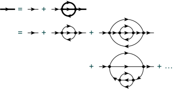
Figure 8: Self-consistency equation for the Fermion propagator (top) and some typical diagrams that make up the full propagator (bottom). Thin lines indicate the bare propagator and thick lines the full (resummed) propagator.

We now come back to the question of evaluating the Fermion Green function

$${\cal G}_{f}({\bf k})=\sum_{k}[\omega-\epsilon_{\bf k}-\Sigma_{f}(\omega)]^{-1},$$ (19)

where $\epsilon_{\bf k}=-J\,\gamma_{\bf k}-\mu$ is the bare dispersion and $\Sigma_{f}(\omega)$ is the Fermion self-energy that arises due to interaction with other Fermions. To make progress, we begin by considering the non-crossing approximation. As before, for the case of the doublon self-energy, we are interested in the high frequency part of the Green functions, and therefore (in the non-crossing approximation) we are justified in replacing the vertices by their momentum averaged counterparts as listed in first row of Table 1, and then working with momentum averaged Green functions and self-energies. In the non-crossing approximation, the Fermion self-consistency equation is depicted diagrammatically in Fig. 8, where the thick Fermion lines represent fully dressed Fermion Green functions that are being determined self-consistently. The Fermion self-energy equations are given by

$$\Sigma_{f}^{{}^{\prime\prime}}(\omega) = -2zJ_{1}^{2}\int_{0}^{\omega}\frac{d\omega^{\prime}}{\pi}S^{{}^{\prime\prime}}(\omega^{\prime})G^{{}^{\prime\prime}}(\omega-\omega^{\prime})$$ (20)

$$\Sigma_{f}^{{}^{\prime}}(\omega) = -2zJ_{1}^{2}\int_{-\infty}^{0}\frac{d\omega^{\prime}}{\pi}S^{{}^{\prime\prime}}(\omega^{\prime}){\cal G}_{f}^{{}^{\prime}}(\omega-\omega^{\prime})$$ (21)

$$\quad+2zJ_{1}^{2}\int_{0}^{\infty}\frac{d\omega^{\prime}}{\pi}{\cal G}_{f}^{{}^{\prime\prime}}(\omega^{\prime})S^{{}^{\prime}}(\omega-\omega^{\prime}).$$

Combining these self-energy equations with the definition of the Green function Eq. (19), we obtain a set of self-consistent equations for the Fermion Green function.

IV.3 Corrections Due to Diagrams Left Out

Figure 9: Typical crossed fermion diagrams that are missed by the resummation method. These types of diagrams are expected to strongly contribute to the Fermion self-energy at high frequencies and therefore to the doublon decay rate.

Figure 10: Typical type III diagrams that are missed by the resummation method. As explained in the main text, these diagrams are expected to give some contribution to the doublon self-energy, but their effect is not taken into account.

In the resummation formalism we have missed three important classes of diagrams: type I diagrams, which correspond to doublon self-energy diagrams with crossing Fermion lines (examples depicted in Fig. 7); type II diagrams, which are Fermion self-energy diagrams with crossing Fermion lines (examples depicted in Fig. 9); and type III diagrams, which are doublon self-energy diagrams which are left out and are neither type I nor type II (examples depicted in Fig. 10).

As mentioned earlier, we have empirically checked that type I diagrams do not contribute to the doublon self-energy due to the lack of pairing of the Fermion-doublon vertex factors. However, there are no similar arguments for excluding type II or type III diagrams. We suppose that when a doublon emits a particle-hole pair, the particle and hole are not coherent with each other, and therefore, we make the approximation of dropping type III diagrams. However, each Fermion in the emitted pair still interacts with the Fermi sea, resulting in both non-crossing Fermion self-energy diagrams, that have already been taken care of, and type II diagrams which we shall try to estimate.

Since we cannot evaluate all the type II diagrams explicitly, we proceed to approximate their effect on the Fermion self-energy in the following way:

(a) We assume that at a given frequency $\omega$, the leading contribution to the imaginary part of self-energy $\text{Im}\;\Sigma_{f}(\omega)$ comes from diagrams of a definite order $n_{0}(\omega)$, as diagrams of lower order do not have enough particle-hole pairs to absorb $\omega$ and diagrams of higher order are suppressed by additional powers of $J/\omega$. We expect $n_{0}(\omega)$ to scale linearly with $\omega$ as the main contribution to the spectral function at $\omega$ comes from exciting $\sim\omega/\epsilon_{0}$ particle-hole pairs, where $\epsilon_{0}$ is the typical energy of particle-hole pairs.

(b) To determine $n_{0}(\omega)$, we keep the Fermion-Fermion vertex energy scale $J_{1}$ as a free parameter, and calculate $n_{0}(\omega)$ from the logarithmic derivative

$$n_{0}(\omega)=\frac{1}{2}\left.\frac{d\log\Sigma_{f}(\omega)}{d\log J_{1}}\right|_{J_{1}=J}.$$ (22)

This relation is exact if only one order of diagrams contribute at given energy; for the case of different orders contributing to self-energy, this gives a number close to the order with leading contribution. $n_{0}(\omega)$, obtained from the resummed self-energy, is plotted in Fig. (11). The best fit for this graph is $n_{0}(\omega)=\omega/(5.85J)-1/2$.

(c) We then compute the ratio of the total number of possible $n^{\text{th}}$ order Fermion self-energy diagrams to the number of $n^{\text{th}}$ order diagrams included in the resummation scheme, $R(n)$. $R(n)$ can then be interpolated to form a function of the continuous variable $n$. See Appendix C for details of computing this ratio.

(d) In the final step, we rescale the imaginary part of the Fermion self-energy by $R(n_{0}(\omega))$ to obtain a better approximation including effects of missed diagrams

$$\Sigma_{f}^{{}^{\prime\prime}}(\omega)\rightarrow\Sigma_{f}^{{}^{\prime\prime}}(\omega)R[n_{0}(\omega)].$$ (23)

Here, we are making an assumption: the amplitude of the Fermion self-energy diagram only depends on its order in perturbation theory and not on the details of the structure of the diagram. Modulo the contribution of the type III diagrams, this approximation should overestimate the decay rate as the crossing diagrams usually contribute less than the non-crossing diagrams due to the momentum sums involved.

To complete the calculation of the doublon self-energy, we use the Fermion Green function to construct the particle-particle and particle-hole propagators Eqs. (15-18), which appear in the self-energy equations for the doublon Eqs. (13, 14).

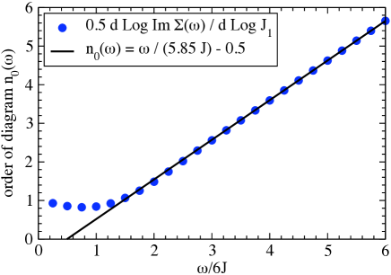
Figure 11: Order with largest contribution to the Fermion self-energy $n_{0}(\omega)$ as a function of the frequency $\omega$. The solid line represents the best linear fit for the high frequency data.

V Theoretical Results and Comparison with Experiments

In this section we look at the theoretical results of the doublon lifetime calculation and compare them with experimental results. We start by summarizing the method of calculation, which will help in establishing different approximation schemes. We then discuss the results from different schemes and their comparison with experiments.

The calculation of the decay rate via the resummation technique has two important steps. The first one is the evaluation of the Fermion Green’s functions which are used to compute the particle-particle and particle-hole propagators. The second one is the evaluation of the doublon self-energy, which uses these propagators. As mentioned before, a non-crossing approximation for the doublon self-energy yields good results. The crossing diagrams give negligible contribution as the vertex functions which oscillate with momenta kills the momentum averages. We also note that there is a set of doublon self-energy diagrams (the type III diagrams) which we neglect in our calculation.

Our approximations are then related to different ways of evaluating the Fermion propagators. We consider three different approximations: (i) Non-interacting Fermions; in this case we use the free Fermion propagators with a band dispersion. One way of looking at this approximation is to set $J_{1}=0$. (ii) Non-crossing approximation for interacting Fermions; in this case we set $J_{1}=J$ but use only non-crossing diagrams to evaluate the Fermion propagators. (iii) Modified self-energy for interacting Fermions; in this case we modify the self-energy of the interacting Fermions obtained by non-crossing approximation to take into account Fermion self-energy diagrams missed in the resummation. The modification procedure is detailed in the previous Section.

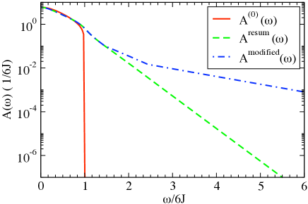
Figure 12: Fermion spectral functions in different approximations: the free Fermion spectral function ($A^{(0)}(\omega)$); the projected Fermion spectral function obtained as the result of the resummation procedure ($A(\omega)$); the projected Fermion spectral function including corrections for missing diagrams in the resummation procedure (corrected $A(\omega)$). The linear slope at high energies on a semi-logarithmic scale shows the exponential transfer of spectral weight due to projection induced interactions.

We plot the spectral function of the Fermions, $A(\omega)=-(1/\pi)\text{Im}{\cal G}_{f}(\omega)$, for the three approximations in Fig. 12. In the non-interacting case, this is simply the density of states in a cubic lattice and the spectral weight is zero outside the band. In the non-crossing approximation, we see that there is a transfer of spectral weight from low energies to an exponential tail at high energies, which reflects the fact that interaction induced by projection leads to the possibility of creating a high energy Fermion, which can reduce its energy by creating particle-hole pairs. This is an important qualitative change that affects the physics of doublon decay in a fundamental way. The interacting Fermion approximation allows two distinct decay processes : (a) creation of several low energy ($\omega\sim 2zJ$) particle-hole pairs and (b) creation of a high energy particle-hole pair which then decays into a shower of low energy particle-hole pairs. The second process is forbidden for non-interacting Fermions. Finally, in the modified self-energy approximation, we include more processes to create particle-hole pairs and hence there is a larger shift of spectral weight to higher energies, as evidenced by the slower decay of the tail. This enhances the importance of the (b) channel for decay.

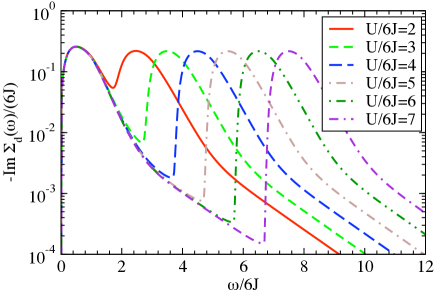
Figure 13: Doublon self-energy (in the modified Fermion self-energy approximation) for various values of $U/6J$.

In the second step we use the Fermion propagator obtained in step one to self-consistently compute the doublon self-energy. The imaginary part of the doublon self-energy for various $U/6J$ ratios is depicted in Fig. 13. The main features are a pair of peaks, one occurring at small frequencies, and another at high frequencies. As there are no excitations in the Fermi system in the initial state, for frequencies $\omega\leq U$ a nonzero value of $\text{Im}\Sigma_{d}(\omega)$ corresponds directly to the rate of doublon decay. At low frequencies, the doublon is far from its mass shell and rapidly decays into a pair of particles. As the frequency increases more and more particle-hole pairs are required to absorb the doublon energy resulting in the exponential decrease in $\text{Im}\Sigma_{d}(\omega)$. As $\omega$ surpasses $U$, a new contribution to the imaginary part of the doublon self-energy arises from processes where the doublon can scatter into a lower energy state closer to the mass shell by releasing the excess energy in the form of a few particle-hole excitations. This scattering process is responsible for the high frequency peak in $\text{Im}\Sigma_{d}(\omega)$, that starts growing at $\omega=U$. As we are interested in the decay of a doublon on the mass shell, we read it from $\text{Im}\Sigma_{d}(U)$, which corresponds to the smallest value of $\text{Im}\Sigma_{d}(\omega)$ between the two peaks.

Figure 14: Doublon decay time as a function of $U/6J$. The blue circles are the experimental data (cf. Fig. 4). The lines represent theoretical results from resummation with different levels of sophistication from non-interacting Fermions (red dashed line) to the non-crossing approximation with interacting Fermions (green dot-dashed line) to the modified self-energy approximation (purple solid line).

In Fig. 14, we plot the experimentally obtained decay time together with the theoretical estimates from the three different approximations mentioned earlier. We proceed in the order of sophistication, starting from the non-interacting Fermion case. We see that the decay time obtained with non-interacting Fermions ($J_{1}=0$) via resummation of doublon self-energy diagrams is much longer than the experimentally obtained one. Setting $J_{1}=J$, and using non-crossing diagrams for Fermion self-energy, we obtain a decay time that is a closer match to the experimental data, but is still too long. Next, we take care of the corrections to the imaginary part of the Fermion self-energy from crossing diagrams and find a reasonable match with experiments.

Finally, we want to comment on the remaining free parameters in our calculation. The chemical potential of the Fermions, which determine the hole density, is a free parameter, which can in principle be determined from an equilibrium theory of a strongly interacting doped Hubbard model. Since there is no consensus about the theory of the doped Hubbard model, we prefer to keep it as a free parameter. We vary it within the plausible range of $0.25J$ to $(-0.3J)$ to see how sensitive our results are to the choice of this parameter. The dispersion in the lifetime is then plotted as the shaded region in Fig. 4. We see that we find good quantitative agreement with the experiments in the slope of the lifetime curve, i.e. for the co-efficient $\alpha$ in the exponent of the scaling function. The agreement in the prefactor $C$ is also fair, but this quantity is sensitive to the choice of the free parameter in our calculation.

VI Concluding Remarks

We have studied the decay of artificially created double occupancies in the repulsive Fermi-Hubbard model in the presence of a background compressible state. The situation is experimentally realized by creating double occupancies and corresponding holes on top of a half-filled system via optical lattice modulation. Experimentally it is found that the decay time of the doublons scales exponentially with $U/J$. We can understand the observed scaling in terms of the fact that in order to decay the doublon has to distribute its energy ($\sim U$) among $\sim U/J$ particle-hole excitations. We have developed a detailed theoretical description of this process using diagrammatic resummation techniques. Although the scaling form can be understood from a simple energy conservation argument, we find that the co-efficient in the exponent depends substantially on the strong interaction between the background Fermions. After taking into account the effects of these strong interactions, we find quantitatively fair agreement between theory and experimental results.

The exponentially large lifetime of the doublons has serious implications for use of cold atom systems to simulate the equilibrium properties of the Hubbard model at large values of $U/J$. Typically, in cold atom experiments, the strong interaction regime of the Hubbard model is accessed by cooling the atoms in a weakly interacting state and then tuning either the optical potential or the magnetic field to change $U/J$. The lifetime of the doublons constrains the maximum sweep rate of these Hamiltonian parameters under which thermal equilibrium is maintained. As one goes towards larger $U/J$, the sweep rates need to be exponentially slow to maintain thermodynamic adiabaticity. Given intrinsic constraints like lifetime of a sample, this would restrict the values of $U/J$ for which the simulation of Hubbard model in thermal equilibrium can be achieved.

However, this also opens up the possibility of studying non-equilibrium dynamics of the Hubbard model, which may contain interesting and new physics. In addition, the long lifetime of the doublons also leads to the possibility of observing metastable states with finite density of doublons. An intriguing scenario is observing $\eta$ pairing of doublons and holes etapair .

Finally, we point out that similar phenomena may be relevant to the issues of equilibration in the Bosonic Hubbard model. In a recent paper Chin2009 C. Chin’s group observed the equilibration of the density distribution of Bosonic atoms in a two dimensional optical lattice after the lattice potential was ramped up. As the system relaxed toward equilibrium, the center of the trap heated up, which required the increase in the number of doublons. The slow relaxation timescale observed in experiments may be a reflection of the “dual” problem to the one we discussed in this paper: slow rate of formation of doublons from a a state containing only singly occupied sites and holes.

VII Acknowledgements

We would like to thank A. Georges, A. Rosch, L. Glazman, and C. Chin for useful discussions. R.S., D.P., and E.D. acknowledge the financial support of NSF, DARPA, MURI and CUA. E.A. acknowledges support from BSF (E.D. and E.A.) and ISF. The experimental work was supported by SNF, NAME-QUAM (EU) and SCALA (EU).

Appendix A Model

In this appendix we derive the model we use to describe doublon decay in the background of a projected Fermi sea. We begin with the Fermi-Hubbard model

$$H_{\text{FH}}=-J\sum_{\langle ij\rangle\sigma}c^{\dagger}_{i,\sigma}c^{\phantom{\dagger}}_{j,\sigma}+U\sum_{i}n_{i,\uparrow}n_{i,\downarrow},$$ (24)

where the first term describes the hopping of fermions and the second term the on-site repulsive interaction. We are interested in the case $U\gg J$, where we expect doublons to be meta-stable particles. Therefore, our goal is to decouple the doublon sector from the sector of singles. We do this by projecting out double occupancies from the singles sector, and introducing doublon creation and annihilation operators $d^{\dagger}_{i}$ and $d_{i}$ to take their place. We, proceed in two steps, first we use projection operators to separate the terms in the Fermi-Hubbard Hamiltonian that preserve the number of doublons from those that change it:

$$H_{\text{FH}}=H_{0}+H_{+1}+H_{-1},$$ (25)

where $H_{0}$ preserves the number of doublons

$$H_{0} =-J\sum_{\langle ij\rangle\sigma}(1-n_{i\bar{\sigma}})c^{\dagger}_{i\sigma}c^{\phantom{\dagger}}_{j\sigma}(1-n_{j\bar{\sigma}})$$

$$-J\sum_{\langle ij\rangle\sigma}(n_{i\bar{\sigma}})c^{\dagger}_{i\sigma}c^{\phantom{\dagger}}_{j\sigma}(n_{j\bar{\sigma}})$$

$$+U\sum_{i}n_{i\uparrow}n_{i\downarrow},$$ (26)

and $H_{\pm 1}$ increases/decreases it by one

$$H_{+1} =-J\sum_{\langle ij\rangle\sigma}(n_{i\bar{\sigma}})c^{\dagger}_{i\sigma}c^{\phantom{\dagger}}_{j\sigma}(1-n_{j\bar{\sigma}}),$$ (27)

$$H_{-1} =-J\sum_{\langle ij\rangle\sigma}(1-n_{i\bar{\sigma}})c^{\dagger}_{i\sigma}c^{\phantom{\dagger}}_{j\sigma}(n_{j\bar{\sigma}}),$$ (28)

where $n_{i\sigma}=c^{\dagger}_{i\sigma}c^{\phantom{\dagger}}_{i\sigma}$ and $\bar{\sigma}$ indicates spin opposite to $\sigma$. In the second step, we replace double occupancies by the corresponding doublon operators. Thus we have

$$H_{0}= -J\sum_{\langle ij\rangle\sigma}(1-n_{i\bar{\sigma}})(1-n^{d}_{i})c^{\dagger}_{i\sigma}c^{\phantom{\dagger}}_{j\sigma}(1-n^{d}_{j})(1-n_{j\bar{\sigma}})$$

$$-J\sum_{\langle ij\rangle\sigma}d^{\dagger}_{i}d^{\phantom{\dagger}}_{j}c^{\phantom{\dagger}}_{i\sigma}c^{\dagger}_{j\sigma}+U\sum_{i}n^{d}_{i},$$ (29)

and

$$H_{+1} =-J\sum_{\langle ij\rangle\sigma}\sigma d^{\dagger}_{j}(c_{j\bar{\sigma}}c_{i\sigma})(1-n_{i\bar{\sigma}})$$ (30)

$$H_{-1} =-J\sum_{\langle ij\rangle\sigma}\sigma(1-n_{i\bar{\sigma}})(c^{\dagger}_{i\sigma}c^{\dagger}_{j\bar{\sigma}})d_{j},$$ (31)

where $n^{d}_{i}=d^{\dagger}_{i}d^{\phantom{\dagger}}_{i}$. Thus far, we have obtained an expression for the Fermi-Hubbard Hamiltonian that incorporates doublon operators. This Hamiltonian was specifically derived in such a way as to avoid creation of spurious states (e.g. a doublon and a single fermion on the same site) by the use projection operators. As a result, we do not need to supplement it with a constraint equation.

Now we can separate the terms in the Hamiltonian based on which sectors they connect. The Fermion-Fermion term arises from terms in $H_{0}$ that connect the projected sector and is given by

$$H_{f}=-J\sum_{\langle ij\rangle\sigma}(1-n_{i\bar{\sigma}})c^{\dagger}_{i\sigma}c^{\phantom{\dagger}}_{j\sigma}(1-n_{j\bar{\sigma}}).$$ (32)

Likewise, the Doublon repulsion term also arises from $H_{0}$ and is given by

$$H_{d}=U\sum_{i}n^{d}_{i}.$$ (33)

The remaining terms connect the Fermion and Doublon sectors and are

$$H_{fd} =H_{+1}+H_{-1}+J\sum_{\langle ij\rangle\sigma}$$ (34)

$$\left[(1-n_{i\bar{\sigma}})n^{d}_{j}+n^{d}_{i}(1-n_{j\bar{\sigma}})+d^{\dagger}_{j}d^{\phantom{\dagger}}_{i}\right]c^{\dagger}_{i\sigma}c^{\phantom{\dagger}}_{j\sigma},$$ (35)

where we have dropped the term that is nonzero in the presence of a pair of doublons as we are assuming that there is at most one doublon. To complete the model, we drop terms that result in Feynman vertices with more than two incoming and two outgoing propagators. We have verified, numerically, that these diagrams do not significantly contribute to the doublon decay rate.

Appendix B Checks on Approximations through Fermi Golden Rule Calculation

In this appendix, we compute the doublon decay rate for the case of non-interacting Fermions (i.e., we disregard $H_{p}$ part of the Hamiltonian (8)). We treat $H_{0}=H_{f}^{0}+H_{d}$ as the base Hamiltonian, and $H_{fd}$ as the perturbation Hamiltonian, and evaluate the decay rate, via the Golden Rule, to very high order in $H_{fd}$ using Monte Carlo integration. The objective of this appendix is to test the approximations made in the resummation technique of Section IV on a simplified Hamiltonian. In particular, we empirically verify that (1) we may ignore the crossing diagrams in doublon self-energy and (2) we can use momentum averaged Green functions to compute the decay rates. We begin by laying out the formalism, and then list the results of Monte Carlo integration of decay rates.

B.1 Formalism

Our goal is to compute the transition rate from the starting configuration composed of a single doublon in a Fermi sea at finite temperature to the final configuration composed of the initial Fermi sea with the doublon converted into a pair of single particles and a number of particle-hole excitations. The Fermi Golden rule states that the decay rate is given by

$$\Gamma(p)=\frac{2\pi}{\hbar}\sum_{f}|\langle i|T|f\rangle|^{2}\delta(E_{i}-E_{f}),$$ (36)

where the matrix element can be expressed in ordinary perturbation theory via

$$\langle f|T|i\rangle\!\!=\!\!\!\!\sum_{s_{1},s_{2},...}\!\!\frac{\langle f|H_{fd}|s_{n-1}\rangle\langle s_{n-1}|H_{fd}|s_{n-2}\rangle...\langle s_{1}|H_{fd}|i\rangle}{(E_{i}-E_{s_{1}})(E_{i}-E_{s_{2}})...(E_{i}-E_{s_{n-1}})}.$$ (37)

Here, the sum goes over all intermediate states $s_{i}$, with energy $E_{s_{i}}$, and $n$ is the order of perturbation theory. In this perturbation theory, the action of $H_{fd}$ (except for the final matrix element $\langle f|H_{fd}|s_{n-1}\rangle$) is to create particle-hole pairs. In principle, we may be able to connect the initial state to the final state via other processes, e.g. doublon$\rightarrow$particle-particle$\rightarrow$doublon, however, these process lead to decay at higher order in perturbation theory, and thus we ignore them.

We label the initial state by the momentum of the doublon $p$:

$$|i\rangle=|\cdot;p\rangle=d^{\dagger}_{p}|\text{FS}\rangle.$$ (38)

Likewise, we label the final state via a set of momenta for the up (down) spin particles $k_{i\uparrow(\downarrow)}$ and the up (down) spin holes $q_{i\uparrow(\downarrow)}$:

$$|f\rangle =\left|\begin{array}[]{cc}k_{1,\uparrow}...k_{n_{\uparrow}+1,\uparrow},&k_{1,\downarrow}...k_{n_{\downarrow}+1,\downarrow},\\ q_{1,\uparrow}...q_{n_{\uparrow},\uparrow},&q_{1,\downarrow}...q_{n_{\downarrow},\downarrow}\end{array};\cdot\right\rangle$$ (41)

$$=c^{\dagger}_{k_{n_{\uparrow}+1,\uparrow}}c^{\dagger}_{k_{n_{\downarrow}+1,\downarrow}}\left(c^{\dagger}_{k_{n_{\downarrow},\downarrow}}c_{q_{n_{\downarrow},\downarrow}}\right)...\left(c^{\dagger}_{k_{1,\downarrow}}c_{q_{1,\downarrow}}\right)\times$$

$$\quad\quad\quad\times\left(c^{\dagger}_{k_{n_{\uparrow},\uparrow}}c_{q_{n_{\uparrow},\uparrow}}\right)...\left(c^{\dagger}_{k_{1,\uparrow}}c_{q_{1,\uparrow}}\right)|\text{FS}\rangle,$$ (42)

where $n_{\uparrow\,(\downarrow)}$ counts the number of spin up (down) particle-hole pairs created ($n_{\uparrow}+n_{\downarrow}+1=n$).

The intermediate states are composed of a doublon and $1,2,3,...,n-1$ fermion-hole pairs. Using $H_{fd}$, we can write the matrix element as

$$\langle f|T|i\rangle =\left\langle\begin{array}[]{cc}k_{1,\uparrow}...k_{n_{\uparrow}+1,\uparrow},&k_{1,\downarrow}...k_{n_{\downarrow}+1,\downarrow},\\ q_{1,\uparrow}...q_{n_{\uparrow},\uparrow},&q_{1,\downarrow}...q_{n_{\downarrow},\downarrow}\end{array};\cdot\right|T\left|\cdot;p\right\rangle$$ (45)

$$=\sum_{\text{permutations}}\text{sig}(\text{perm})\frac{\langle f|H_{1}|(\tilde{\sigma}_{1},\tilde{k}_{1},\tilde{q}_{1}),...,(\tilde{\sigma}_{n-1},\tilde{k}_{n-1},\tilde{q}_{n-1});\tilde{p}_{n-1}\rangle...\langle(\tilde{\sigma}_{1},\tilde{k}_{1},\tilde{q}_{1});\tilde{p}_{1}|H_{1}|p\rangle}{(\xi_{\tilde{k}_{1}}+...+\xi_{\tilde{k}_{n-1}}-\xi_{\tilde{q}_{1}}-...-\xi_{\tilde{q}_{n-1}})...(\xi_{\tilde{k}_{1}}+\xi_{\tilde{k}_{2}}-\xi_{\tilde{q}_{1}}-\xi_{\tilde{q}_{2}})(\xi_{\tilde{k}_{1}}-\xi_{\tilde{q}_{1}})},$$ (46)

where $\tilde{k}_{i}$, $\tilde{q}_{j}$, $\tilde{p}_{v}$ stand for the particle, hole, and doublon momenta, respectively, and $\tilde{\sigma}_{i}$ indicates the spin of the $i$-th particle-hole pair. The sum runs over all intermediate states that lead to the final state $|f\rangle$. That is, we must sum over all permutations of assigned values to $(\tilde{\sigma}_{i},\tilde{k}_{i},\tilde{q}_{j})$ from the list $\{k_{1,\uparrow},...,k_{n_{\uparrow}+1}\}$, $\{k_{1,\downarrow},...,k_{n_{\downarrow}+1}\}$, $\{q_{1,\uparrow},...,q_{n_{\uparrow}}\}$, $\{q_{1,\downarrow},...,q_{n_{\downarrow}}\}$. Within this labeling scheme, the doublon momenta in the intermediate states $\tilde{p}_{v}$, and the hole momentum in the final state, are chosen automatically by momentum conservation. We take care of the Fermionic anti-commutation relations with $\text{sig}(\text{perm})$, which stands for the signature of the permutation, and is $\pm 1$ for even/odd permutations of momenta.

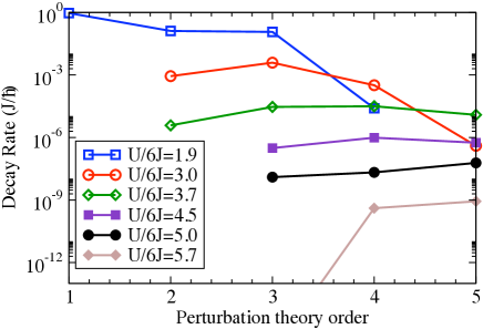
Figure 15: Decay rate as a function of the order of the perturbation theory computed using Fermi Golden rule. Largest decay rate corresponds to most important order.

To obtain the decay rate, we trace over the final states, order by order in perturbation theory,

$$\Gamma(p)=\sum_{n=0}^{\infty}\Gamma^{n}(p).$$ (47)

At each order we trace over the number of up- and down-spin particle-hole pairs, and the corresponding momenta of particles and holes that make up the final state. The decay rate at $n$-th order is the given by the expression

$$\Gamma^{n}(p)=\frac{2\pi}{\hbar}\sum_{n_{\uparrow}+n_{\downarrow}+1=n}\int\frac{\left[{d\!\bar{}\,}k_{1,\uparrow}...{d\!\bar{}\,}k_{n_{\uparrow}+1,\uparrow}\right]\,\left[{d\!\bar{}\,}k_{1,\downarrow}...{d\!\bar{}\,}k_{n_{\downarrow}+1,\downarrow}\right]\,\left[{d\!\bar{}\,}q_{1,\uparrow}...{d\!\bar{}\,}q_{n_{\uparrow},\uparrow}\right]\,\left[{d\!\bar{}\,}q_{1,\downarrow}...{d\!\bar{}\,}q_{n_{\downarrow},\downarrow}\right]}{(n_{\uparrow}+1)!(n_{\downarrow}+1)!(n_{\uparrow})!(n_{\downarrow})!}$$

$$\quad\quad\quad\quad\quad\quad\quad\quad\quad\delta(U-E_{f})\,\delta\left(p-\sum k+\sum q\right)\left|\left\langle\begin{array}[]{cc}k_{1,\uparrow}...k_{n_{\uparrow}+1,\uparrow},&k_{1,\downarrow}...k_{n_{\downarrow}+1,\downarrow},\\ q_{1,\uparrow}...q_{n_{\uparrow},\uparrow},&q_{1,\downarrow}...q_{n_{\downarrow},\downarrow}\end{array};\cdot\right|T\left|\cdot;p\right\rangle\right|^{2},$$ (50)

where ${d\!\bar{}\,}k$ stands for $f(k)\,d^{3}k/(2\pi)^{3}$, ${d\!\bar{}\,}q$ for $(1-f(q))\,d^{3}q/(2\pi)^{3}$, and $f(k)$ is the Fermi function. The denominator in the integral takes care of the fact that interchanging a pair of momentum labels does not change the final state, $E_{f}=\xi(k_{1,\uparrow})+...+\xi(k_{n_{\uparrow}+1,\uparrow})+\xi(k_{1,\downarrow})+...+\xi(k_{n_{\downarrow}+1,\downarrow})-\xi(q_{1,\uparrow})-...-\xi(q_{n_{\uparrow},\uparrow})-\xi(q_{1,\downarrow})-...-\xi(q_{n_{\downarrow},\downarrow}))$ is the final state energy, and the second $\delta$ function takes care of momentum conservation.

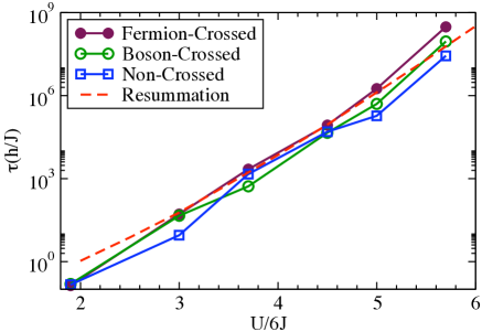
Figure 16: Comparison of the resummation method and various Golden Rule approximations for calculating the dependence of the Doublon decay time on the interaction strength $U/6J$ (with non-interacting Fermions).

We explicitly evaluate the $3^{2n}$ dimensional integral in Eq. (50) numerically via Monte Carlo integration. To perform this integration, we replace the $\delta$ function of energy, which defines a hypersurface in momentum space – a volume of of measure zero, by the top hat function. We also use important sampling to speed up integration by biasing our selection so that we pick particle-hole pairs with holes in the Fermi sea and particles outside of it. The main numerical constraint on the speed of integration comes from evaluating the $(n_{\uparrow}+1)!(n_{\downarrow}+1)!n_{\uparrow}!n_{\downarrow}!$ permutations over the intermediate states, which becomes rather expansive for $n>6$.

B.2 Results

We begin by verifying that the perturbation theory in $H_{fd}$ does indeed converge. That is, for fixed $U/6J$, does $\Gamma^{(n)}(p)$ decrease sufficiently fast as $n$ increases? We know that for $n\lesssim U/12J$, $\Gamma^{(n)}(p)=0$, as not enough particle-hole pairs are formed to carry away the energy of a doublon. When $n\sim U/12J$, in order to satisfy energy conservation, particles created in the decay must have momentum in vicinity of the band maximum near $(\pi,\pi,\pi)$ and holes in the vicinity of the band minimum at $(0,0,0)$. Therefore, for $n\sim U/12J$ the volume of the momentum space being integrated is very small, but this volume increases quickly as $n$ grows. As a result, we expect that the $\Gamma^{(n)}(p)$ will increase with $n$ for small $n$. On the other hand, at high orders the decay rate is suppressed by a high powers of the small parameter $J/U$. Thus, we expect $\Gamma^{(n)}(p)$ to have a maximum for some intermediate value of $n$ close to, but somewhat larger than $U/12J$.

In Fig. 15 we plot $\Gamma^{(n)}(p)$ as a function of $n$ for various values of $U/6J$. In all cases, computations have been performed at $T=0$ and $\mu=0$ (corresponding to one particle per two sites). As expected, in all cases, we see a clear peak in $\Gamma^{(n)}(p)$ at $n\sim U/12J+2$.

Having verified the convergence of the high order perturbation expansion, we move on to empirically verify whether we can ignore crossing diagrams, at least for the case of free Fermions. In order to perform this comparison we compute the total decay rate as a function of $U/6t$ using both Monte Carlo integration of Eq. (50) (incorporates all possible diagrams), as well as the resummation of the non-crossing diagrams given by Eq. (14) with bare Fermion Green functions used to compute $C(\omega)$ and $S(\omega)$. We perform two additional tests using Monte Carlo integration: (1) We calculate the decay rate with Bosonic instead of Fermionic signs for closed Fermion loops; (2) We keep only the diagonal terms, i.e. we replace $|\sigma_{\text{perm}}...|^{2}\rightarrow\sigma_{\text{perm}}|...|^{2}$, which corresponds to the order-by-order summation of non-crossing diagrams, but without momentum averaging of the resummation approach. The results of these four types of calculations are plotted in Fig. 16, for $T=0$ and $\mu=0$. There is very good agreement between all four cases, confirming that crossing diagrams may indeed be dropped as explained in subsection IV.1.

Figure 17: All distinct tree diagrams with one vertex (left) and two vertices (right).

Appendix C Diagram Counting

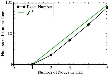
Figure 18: Dependence of the number of distinct tree diagrams on the number of nodes in the tree.

In this appendix we describe the procedure for counting the total number of distinct, spin-labeled Fermion self-energy diagrams at a given order $Q_{\text{all}}(n)$ and the number of non-crossed spin-labeled Fermion self-energy diagrams $Q_{\text{nc}}(n)$. We remind the reader that $Q_{\text{all}}(n)$ and $Q_{\text{nc}}(n)$ correspond to diagrams with $2n$ vertices. For high $\omega$, $\Sigma_{f}^{{}^{\prime\prime}}(\omega)$ is dominated by diagrams with maximal number of particle and hole lines in the middle, as these maximize the energy that is being transferred to the particle-hole pairs being created. In fact, the range in $\omega$ over which $\Sigma_{f}^{{}^{\prime\prime}}(\omega)$ is nonzero is proportional to the number of particle- and hole-lines in the middle of the diagram. Therefore, to simplify the counting, we only count diagrams that have the maximal number ($2n+1$) of particle- and hole-lines going across the middle of the diagram.

To count the number of diagrams at given $n$, we first construct all distinct tree diagrams (without spin labels) that have a single particle going in, $n+1$ particles and $n$ holes going out and $n$ vertices of the type given in first row of Table 1. In Fig. 17, we show all such tree diagrams for $n=1$ and $n=2$. In Fig. 18 we show how the number of distinct trees scales with $n$.

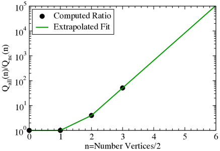
Figure 19: Correction ratio as a function of the order of the diagram.

Next, we construct the set of all the possible self-energy diagrams by taking a pair of tree diagrams, reversing all the arrows in one of them, and gluing them together. When we count the total number of diagrams, we glue together particle-particle lines and hole-hole lines in all pairs of trees at the given order, in all possible ways. On the other hand, when counting the number of diagrams produced by the non-crossing approximation, we only glue together trees with their mirror image. Finally, we spin label the resulting diagrams, and remove all duplicate diagrams, to obtain $Q_{\text{all}}(n)$ and $Q_{\text{nc}}(n)$.

We assume that the ratio $Q_{\text{all}}(n)/Q_{\text{nc}}(n)$ scales like $\sim e^{\alpha n}$. We use this assumption to extrapolate the ratio for non-integer values of $n$ and for large values of $n>4$. We plot the ratio of $Q_{\text{all}}(n)/Q_{\text{nc}}(n)$, along with the extrapolated curve that we use in rescaling the Fermion self-energy, in Fig. 19.

References

- (1) A. B. Linde in Particle Physics and Inflationary Cosmology, Harwood, (1990).
- (2) M. Prakash, M. Prakash, R. Venugopalan and G. Welke, Phys. Rep. 227, 321 (1993)
- (3) G. Müller et. al, Nature Materials, 8, 56 (2009).
- (4) E. H. Lieb and W. Liniger, Phys. Rev. 130, 1605 (1963)
- (5) M. Rigol, V. Dunjko, M. Olshanii, Nature, 452, 854 (2008).
- (6) T. Kinoshita, T. Wenger and D. S. Weiss, Nature, 440, 900 (2006).
- (7) V. Perebeinos and P. Avouris, Phys. Rev. Lett. 101, 057401 (2008).
- (8) G. B. Brown and W. Weise, Phys. Rep. 22, 279 (1975).
- (9) N. Strohmaier et. al, arXiv:0905.2963, accepted for publication in Phys. Rev. Lett.
- (10) R. Sensarma, D. Pekker and E. Demler, in preparation.
- (11) R. Jördens, N. Strohmaier, K. Günter, H. Moritz, T. Esslinger, Nature (London) 455, 204 (2008).
- (12) C. A. Regal, D. S. Jin, Phys. Rev. Lett. 90, 230404 (2003).
- (13) We determine the widths of both resonances by measuring the zero-crossing via dephasing of Bloch oscillations Gustavsson_2008 . This yields G and G, the latter differing from Regal2003 .
- (14) M. Gustavsson et al., Phys. Rev. Lett. 100, 080404 (2008).
- (15) D. Jaksch, C. Bruder, J. I. Cirac, C. W. Gardiner, P. Zoller, Phys. Rev. Lett. 81, 3108 (1998).
- (16) C. Kollath, A. Iucci, I. P. McCulloch, T. Giamarchi, Phys. Rev. A 74, 041604 (2006).
- (17) F. Hassler, S. D. Huber, Phys. Rev. A 79, 021607 (2008).
- (18) S. D. Huber, A. Rüegg, Phys. Rev. Lett. 102, 065301 (2009).
- (19) R. Sensarma, D. Pekker, M. Lukin, E. Demler, Phys. Rev. Lett. 103, 035303 (2009).
- (20) Separate fits to the two spin mixtures yield values of and .
- (21) The pair propagators are momentum integrated objects e.g. and so on
- (22) C. N. Yang, Phys. Rev. Lett. 63, 2144 (1989); A. Rosch, D. Rasch, B. Binz amd M. Vojta, Phys. Rev. Lett. 101, 265301 (2008).
- (23) C.-L. Hung, X. Zhang, N. Gemelke, and C. Chin, arXiv:0910.1382v1.