Robust and Trend-following Kalman Smoothers using Student’s t

Abstract

We propose two nonlinear Kalman smoothers that rely on Student’s t distributions. The T-Robust smoother finds the maximum a posteriori likelihood (MAP) solution for Gaussian process noise and Student’s t observation noise, and is extremely robust against outliers, outperforming the recently proposed $\ell_{1}$-Laplace smoother in extreme situations (e.g. 50% or more outliers). The second estimator, which we call the T-Trend smoother, is able to follow sudden changes in the process model, and is derived as a MAP solver for a model with Student’s t-process noise and Gaussian observation noise. We design specialized methods to solve both problems which exploit the special structure of the Student’s t-distribution, and provide a convergence theory. Both smoothers can be implemented with only minor modifications to an existing $L_{2}$ smoother implementation. Numerical results for linear and nonlinear models illustrating both robust and fast tracking applications are presented.

1 Introduction

The Kalman filter is an efficient recursive algorithm that estimates the state of a dynamic system from measurements contaminated by Gaussian noise (Kalman, 1960). Along with many variants and extensions, it has found use in a wide array of applications including navigation, medical technologies and econometrics (Chui and Chen, 2009; West and Harrison, 1999). Many of these problems are nonlinear, and may require smoothing over past data in both online and offline applications to improve significantly the estimation performance (Gelb, 1974).
In this paper, we focus on two important areas in Kalman smoothing: robustness with respect to outliers in measurement data, and improved tracking of quickly changing system dynamics. Robust smoothers have been a topic of significant interest since the 1970’s, e.g. see (Schick and Mitter, 1994). In order to design outlier robust smoothers, recent reformulations described in (Aravkin et al., 2011b, a; Farahmand et al., 2011) use $L_{1}$, Huber or Vapnik loss functions in place of $L_{2}$ penalties. There have also been recent efforts to design smoothers that are able to better track fast system dynamics, e.g. jumps in the state values. For example, in (Ohlsson et al., 2011) the Laplace distribution is used in place of the Gaussian distribution to model transition noises. This introduces an $L_{1}$ penalty on the state evolution in time and can be interpreted as a dynamic version of the well known LASSO procedure (Tibshirani, 1996).
All of these smoothers can be derived from a statistical point of view, using log-concave densities on process noise, measurement noise, and prior information on the state. Log-concave densities take the form

$${\bf p}(\cdot)\propto\exp(-\rho(\cdot)),\quad\rho\text{ convex}\;.$$ (1.1)

Formulations using (1.1) are nearly ubiquitous, in part because they correspond to convex optimization problems in the linear case. However, to effectively model a regime with large outliers or sudden jumps in the state, we want to look beyond (1.1) in order to allow heavy-tailed distributions.
A particularly convenient heavy-tailed modeling distribution that falls outside of (1.1) is the Student’s t-distribution. In the statistics literature, this distribution was successfully applied to a variety of robust inference applications (Lange et al., 1989), and is closely related to re-descending influence functions (Hampel et al., 1986). In the context of Kalman filtering/smoothing, the idea of using Student’s t-distributions to model both measurement error and innovations (process errors) was studied in (Fahrmeir et al., 1998).
We propose new nonlinear Kalman smoothers which we call T-Robust and T-Trend. For the T-Robust smoother, we model the measurement noise using the Student’s t-distribution, extending the approach in (Aravkin et al., 2011b) to the Student’s t. As a result, errors or ‘outliers’ in the measurements have even less effect on the smoothed estimate, and performs better than (Aravkin et al., 2011b) for cases with high proportion of outliers (e.g. 50% bad data). For the T-Trend smoother, we instead model process noise using the Student’s t-distribution, which allows the smoother to track sudden changes in state.
Our work differs for (Fahrmeir et al., 1998) in two important respects. First, we include nonlinear measurement and process models in our analysis. Second, we propose a novel optimization algorithm to solve both T-Robust and T-Trend smoothing problems. This algorithm differs significantly from the one proposed in (Fahrmeir et al., 1998). In particular, rather than using the Fisher information matrix (i.e. full Hessian), or its expectation as a Hessian approximation (method of Fisher’s scoring) as suggested by (Fahrmeir et al., 1998), we design a modified Gauss-Newton method which builds information about the curvature of the Student’s t-log likelihood into the Hessian approximation, and provide a convergence theory. The fast smoothing procedures proposed here also allow the efficient estimation of hyperparameters such as degrees of freedom (e.g. cross-validation techniques using the EM algorithm are discussed in (Fahrmeir et al., 1998)).
The paper is organized as follows. In section 2 we introduce the multivariate Student’s t-distribution and define the models underlying the T-Robust and T-Trend smoothers. In Section 3 the maximum likelihood objective for T-Robust, the quadratic approximation for this objective, and the convex quadratic program to solve this approximate subproblem are reported. In Section 4 the T-Trend smoother is designed by modeling transitions using Student’s t. We describe our algorithm, provide a convergence theory, and explain the differences with (Fahrmeir et al., 1998) in 5. The T-Robust and T-Trend smoothers are tested using simulated data for linear and nonlinear models in Section 6. We end the paper with some concluding remarks.

2 The T-Robust and T-Trend smoothing problems

Figure 1: Gaussian, Laplace, and Student’s t Densities, Corresponding Negative Log Likelihoods, and Influence Functions (for scalar $v_{k}$).

For a vector $u\in{\mathbb{R}}^{n}$ and any positive definite matrix $M\in{\mathbb{R}}^{n\times n}$, let $\|u\|_{M}:=\sqrt{u^{\rm T}Mu}$. We use the following generalization of the Student’s t-distribution:

$${\bf p}(v_{k}|\mu) = \frac{\Gamma(\frac{s+m}{2})}{\Gamma(\frac{s}{2})\det[\pi sR]^{1/2}}\left(1+\frac{\|v_{k}-\mu\|_{R^{-1}}^{2}}{s}\right)^{\frac{-(s+m)}{2}}$$ (2.1)

where $\mu$ is the mean, $s$ is the degrees of freedom, $m$ is the dimension of the vector $v_{k}$, and $R$ is a positive definite matrix. A comparison of this distribution with the Gaussian and Laplacian distribution appears in Figure 1. Note that the Student’s t-distribution has much heavier tails than the others, and that its influence function is re-descending, see (Maronna et al., 2006) for a discussion of influence functions. This means that as we pull a measurement further and further away, its ‘influence’ decreases to 0, so it is eventually ignored by the model. Note also that the $\ell_{1}$-Laplace is peaked at 0, while the Student’s t-distribution is not, and so a Student’s t-fit will not in general drive residuals to be exactly $0$.
We use the following general model for the underlying dynamics: for $k=1,\ldots,N$

$$\begin{array}[]{ccc}x_{k}&=&g_{k}(x_{k-1})+w_{k}\\ z_{k}&=&h_{k}(z_{k})+v_{k}\end{array}$$ (2.2)

with initial condition $g_{1}(x_{0})=g_{0}+w_{1}$, with $g_{0}$ a known constant, and where $g_{k}:{\mathbb{R}}^{n}\rightarrow{\mathbb{R}}^{n}$ are known smooth process functions, and $h_{k}:{\mathbb{R}}^{n}\rightarrow{\mathbb{R}}^{m(k)}$ are known smooth measurement functions.
For the T-Robust smoother, we assume that the vector $w_{k}\in{\mathbb{R}}^{n}$ is zero-mean Gaussian noise of known covariance $Q_{k}\in{\mathbb{R}}^{n\times n}$, and the vector $v_{k}\in{\mathbb{R}}^{m(k)}$ is zero-mean Student’s t measurement noise (2.1) of known covariance $R_{k}\in{\mathbb{R}}^{m(k)\times m(k)}$ and degrees of freedom $s$.
For the T-Trend smoother, the roles are interchanged, i.e. $w_{k}$ is Student’s t noise while $v_{k}$ is Gaussian. In both cases, we assume that the vectors $\{w_{k}\}\cup\{v_{k}\}$ are all mutually independent.
In the next sections, we design methods to find the MAP estimates of $\{x_{k}\}$ for both formulations.

3 T-Robust smoother

Given a sequence of column vectors $\{u_{k}\}$ and matrices $\{T_{k}\}$ we use the notation

$${\rm vec}(\{u_{k}\})=\begin{bmatrix}u_{1}\\ u_{2}\\ \vdots\\ u_{N}\end{bmatrix}\;,\;{\rm diag}(\{T_{k}\})=\begin{bmatrix}T_{1}&0&\cdots&0\\ 0&T_{2}&\ddots&\vdots\\ \vdots&\ddots&\ddots&0\\ 0&\cdots&0&T_{N}\end{bmatrix}.$$

We also make the following definitions:

$$\begin{array}[]{rcl}R&=&{\rm diag}(\{R_{k}\})\\ Q&=&{\rm diag}(\{Q_{k}\})\\ x&=&{\rm vec}(\{x_{k}\})\end{array}\;,\;\begin{array}[]{rcl}w(x)&=&{\rm vec}(\{x_{k}-g_{k}(x_{k-1})\})\\ v(x)&=&{\rm vec}(\{z_{k}-h_{k}(x_{k})\}).\end{array}$$

Maximizing the likelihood for the model (2.2) is equivalent to minimizing the associated negative log likelihood

$$-\log{\bf p}(\{\nu_{k}\},\{w_{k}\})=-\log{\bf p}(\{\nu_{k}\})-\log{\bf p}(\{w_{k}\})$$

Dropping the terms that do not depend on $\{x_{k}\}$, the objective corresponding to T-Robust is

$$\frac{1}{2}\sum^{N}_{k=1}(s_{k}+m_{k})\log\left[1+\frac{\|v_{k}\|_{R_{k}^{-1}}^{2}}{s_{k}}\right]+\|w_{k}\|_{Q_{k}^{-1}}^{2},$$ (3.1)

where $s_{k}$’s are degrees of freedom parameters associated with measurement noise, and $m_{k}$ are the dimensions of the $k$th observation.

A first-order accurate affine approximation to our model with respect to direction $d={\rm vec}\{d_{k}\}$ near a fixed state sequence $x$ is given by

$$\begin{array}[]{lll}\tilde{w}(x;d)&=&{\rm vec}(\{x_{k}-g_{k}(x_{k-1})-g_{k}^{(1)}(x_{k-1})d_{k}\}),\\ \tilde{v}(x;d)&=&{\rm vec}(\{z_{k}-h_{k}(x_{k})-h_{k}^{(1)}(x_{k})d_{k}\}).\end{array}$$

Set $Q_{N+1}=I_{n}$ and $g_{N+1}(x_{N})=0$ (where $I_{n}$ is the $n\times n$ identity matrix) so that the formulas are also valid for $k=N+1$.

We minimize the nonlinear nonconvex objective in (3.1) by iteratively solving quadratic programming (QP) subproblems of the form:

$$\begin{array}[]{lll}\mbox{min}&\frac{1}{2}d^{\rm T}Cd+a^{\rm T}d\quad\mbox{w.r.t}\;d\in{\mathbb{R}}^{nN},\end{array}$$ (3.2)

where $a$ is the gradient of objective (4) with respect to $x$ and $C$ has the form

$$C=\begin{bmatrix}C_{1}&A_{2}^{\rm T}&0&\\ A_{2}&C_{2}&A_{3}^{\rm T}&0\\ 0&\ddots&\ddots&\ddots&\\ &0&A_{N}&C_{N}\end{bmatrix},$$ (3.3)

with $A_{k}\in{\mathbb{R}}^{n\times n}$ and $C_{k}\in{\mathbb{R}}^{n\times n}$ defined as follows:

$$A_{k} = -Q_{k}^{-1}g^{(1)}_{k}\;,\;$$

$$C_{k} = Q_{k}^{-1}+(g^{(1)}_{k+1})^{\rm T}Q^{-1}_{k+1}g^{(1)}_{k+1}+H_{k}\;,$$

$$H_{k} = \frac{(h_{k}^{(1)})^{\rm T}R_{k}^{-1}h_{k}^{(1)}}{(s_{k}+\|v_{k}\|_{R^{-1}_{k}}^{2})/(s_{k}+m_{k})}\;.$$

The solutions to the subproblem (3.2) have the form $d=-C^{-1}a$, and can be found in an efficient and numerically stable manner in $O(n^{3}N)$ steps, since $C$ is tridiagonal and positive definite (see (Bell et al., 2008)).

4 T-Trend Smoother

The objective corresponding to T-Trend is

$$\frac{1}{2}\sum^{N}_{k=1}(r_{k}+n)\log\left[1+\frac{\|w_{k}\|_{Q_{k}^{-1}}^{2}}{r_{k}}\right]+\|v_{k}\|_{R_{k}^{-1}}^{2},$$ (4.1)

where $r_{k}$ are degrees of freedom parameters associated with process noise, and $n$ is the dimension of each state $x_{k}$. A first-order accurate affine approximation to our model with respect to direction $d={\rm vec}\{d_{k}\}$ near a fixed state sequence $x$ is as follows:

$$\begin{array}[]{lll}\tilde{w}(x;d)&=&{\rm vec}(\{x_{k}-g_{k}(x_{-1})-g_{k}^{(1)}(x_{k-1})d_{k}\}),\\ \tilde{v}(x;d)&=&{\rm vec}(\{z_{k}-h_{k}(x_{k})-h_{k}^{(1)}(x_{k})d_{k}\}).\end{array}$$

As before, we set $Q_{N+1}=I_{n}$ and $g_{N+1}(x_{N})=0$ (where $I_{n}$ is the $n\times n$ identity matrix) so that the formula is also valid for $k=N+1$.

We minimize the nonlinear objective in (4.1) by iteratively solving quadratic programming (QP) subproblems of the form

$$\begin{array}[]{lll}\mbox{min}&\frac{1}{2}d^{\rm T}Cd+a^{\rm T}d\quad\mbox{w.r.t}\;d\in{\mathbb{R}}^{nN},\end{array}$$ (4.2)

where $a$ is the gradient of objective (4) with respect to $x$ and $C$ again has form  (3.3), but now with $A_{k}\in{\mathbb{R}}^{n\times n}$ and $C_{k}\in{\mathbb{R}}^{n\times n}$ defined as follows:

$$A_{k} = -\frac{(r_{k}+n)Q_{k}^{-1}g^{(1)}_{k}}{r_{k}+\|w_{k+1}\|_{Q^{-1}_{k}}^{2}},$$

$$C_{k} = Q_{k}^{-1}+(h_{k}^{(1)})^{\rm T}R_{k}^{-1}h_{k}^{(1)}+H_{k},$$

$$H_{k} = \frac{(g^{(1)}_{k+1})^{\rm T}Q^{-1}_{k+1}g^{(1)}_{k+1}}{(r_{k}+\|w_{k}\|_{Q^{-1}_{k}}^{2})/(r_{k}+n)}.$$ (4.3)

The solutions to the subproblem (4.2) again have the form $d=-C^{-1}a$, where $C$ is tridiagonal and positive definite, so that they still can be found in an efficient and numerically stable manner in $O(n^{3}N)$ steps, see (Bell et al., 2008).

5 Algorithm and Global Convergence

When models $g_{k}$ and $h_{k}$ are all linear, we can compare the algorithmic scheme proposed in the previous sections with the method in (Fahrmeir et al., 1998). The method in (Fahrmeir et al., 1998) proposes using the Fisher information matrix in place of the matrix $C$ above. When the densities for $w_{k}$ and $v_{k}$ are Gaussian, this is equivalent to the Gauss-Newton method. However, in the Student’s t-case, the Fisher information matrix may be indefinite.
When this occurs, (Fahrmeir et al., 1998) propose to use the expectation of the Fisher information matrix, i.e. the Fisher scoring method. In this approach the expected value of $C$ replaces the terms $\|w_{k}\|_{2}^{2}$ or $\|v_{k}\|_{2}^{2}$ in the denominators of $H_{k}$ and $A_{k}$ with their expectations, which are only functions of $s_{k}$ and $r_{k}$, the degrees of freedom. The crucial difference here is that in practice, we want to pass the information about which $\|w_{k}\|$ and $\|v_{k}\|$ are large to the algorithm, so that it can curtail their contribution to the model updates. So while the Fisher information matrix is too unstable (can become indefinite), the expected Fisher information is insensitive to the magnitude variations the algorithm should incorporate as it proceeds.
For these reasons, we propose a Gauss-Newton method which uses the relative size information of the residuals to find the directions of descent, and provide a proof of convergence for the application of this method to solve (3.1). This objective takes the form $K=\rho\circ F$, with the convex function $\rho$ and the smooth function $F$ given by

$$\rho\left(\begin{array}[]{c}c\\ u\end{array}\right) = c+\frac{1}{2}\|u\|_{A^{-1}}^{2}$$ (5.3)

$$F(x) = \left(\begin{array}[]{c}f(x)\\ r(x)\end{array}\right)$$ (5.6)

$$f(x) = \frac{1}{2}\sum_{k=1}^{N}(b_{k}+l_{k})\log\left[1+\frac{\|p_{k}(x)\|_{B_{k}^{-1}}^{2}}{b_{k}}\right],$$ (5.7)

where $r(x)$ and $p(x)$ are smooth functions of $x$, $A$ and $\{B_{k}\}$ are known positive definite matrices, $b_{k},l_{k}$ are fixed constants, and $c\in{\mathbb{R}}$. This structure covers both T-Robust and T-Trend, where for T-Robust $p_{k}(x)=v_{k}(x)$, $r(x)=w(x)$, $A={\rm diag}[\{Q_{k}\}]$ and $B_{k}=R_{k}$, and for T-Trend $p_{k}(x)=w_{k}(x)$, $r(x)=v(x)$, $A={\rm diag}[\{R_{k}\}]$ and $B_{k}=Q)k$. Note that the range of $f$ is ${\bf R_{+}}$.
The objective $K(x)=\rho\circ F(x)$ is convex composite, since $\rho$ is convex and $F(x)$ is smooth. Our approach exploits this structure by iteratively linearizing $F$ about the iterates $x^{k}$ and solving

$$\begin{array}[]{lll}&\displaystyle\min_{d\in{\mathbb{R}}^{nN}}&\rho(F(x^{k})+F^{(1)}(x^{k})d).\end{array}$$ (5.8)

Rather than requiring interior point methods to solve (5.8) as in (Aravkin et al., 2011b), a single block-tridiagonal solve of the system (3.2) yields descent direction $d$ for the objective $K(x)$. While the details of solving the direction finding subproblem are always problem specific, a general convergence theory for convex-composite methods can be derived to establishes the overall convergence to a stationary point of $K(x)$. The theory required generalizes that of (Aravkin et al., 2011b), and includes both T-Robust and T-Trend formulations. We present the theory and remark on its particular application to the problems of interest. Please see (Aravkin, 2010, Theorem 4.5.2, Corollary 4.5.3) for the proofs.
Recall the first-order necessary condition for optimality in the convex composite problem minimize $K(x)$ is

$$0\in\partial K(x)=\partial\rho\left(F(x)\right)F^{(1)}(x)$$

where $\partial K(x)$ is the generalized subdifferential of $K$ at $x$ Rockafellar and Wets (1998) and $\partial\rho\left(F(x)\right)$ is the convex subdifferential of $\rho$ at $F(x)$ Rochafellar (1970). Elementary convex analysis gives us the equivalence

$$0\in\partial K(x)\quad\Leftrightarrow\quad K(x)=\inf_{d}\rho\left(\;F(x)+F^{(1)}(x)d\;\right)\;.$$

For both T-Robust and T-Trend, it is desirable to modify the objective in (5.8) by including curvature information. We therefore define the difference function

$$\Delta(x,H;d)=\rho\left(\;F(x)+F^{(1)}(x)d\;\right)+\frac{1}{2}d^{\rm T}Hd-K(x)\;,$$ (5.9)

where $H=H(x)$ is positive semidefinite and varies continuously with $x$, and the minimum of $\Delta(x,H;d)$ with respect to direction $d$

$$\Delta^{*}(x,H)=\inf_{d}\Delta(x,H;\;d)\;.$$ (5.10)

Since $\frac{1}{2}d^{\rm T}Hd$ is differentiable at the origin for any $H$, we have $\Delta^{*}(x,H)=0$ if and only if $0\in\partial K(x)$ Burke (1985).
Given $\eta\in(0,1)$, we define a set of search directions at $x$ by

$$D(x,H,\eta)=\left\{d\,\left|\,\Delta(x,H;d)\leq\eta\Delta^{*}(x,H)\right.\right\}\;.$$ (5.11)

Note that if there is a $d\in D(x,H,\eta)$ such that $\Delta(x,H;\;d)\geq-\eta\varepsilon$, then $\Delta^{*}(x,H)\geq-\varepsilon$. These ideas motivate the following algorithm Burke (1985).

Algorithm 5.1

Gauss-Newton Algorithm.

1. Given $x^{0}\in{\mathbb{R}}^{Nn}$ an initial estimate of state sequence, $H_{0}\in{\mathbb{S}}^{n}_{+}$ the initial curvature information, $\varepsilon\geq 0$ an overall termination criteria, $\eta\in(0,1)$ a termination criteria for subproblem, $\beta\in(0,1)$ a line search rejection criteria, $\gamma\in(0,1)$ a line search step size factor. Set the iteration counter $\nu=0$.

2. (Gauss-Newton Step) Find $d^{\nu}$ in the set $D(x^{\nu},H_{\nu},\eta)$ in 5.11. Set $\Delta_{\nu}=\Delta(x^{\nu},H_{\nu};d^{\nu})$ in 5.9 and Terminate if $\Delta_{\nu}\geq-\varepsilon$.

3. (Line Search) Set

   $$\begin{array}[]{lll}t_{\nu}&=&\max\gamma^{i}\\ &\text{s.t.}&i\in\{0,1,2,\cdots\}\;\mbox{ and }\\ &\text{s.t.}&\rho\left(F(x^{\nu}+\gamma^{i}d^{\nu})\right)\leq\rho\left(F(x^{\nu})\right)+\beta\gamma^{i}\Delta_{\nu}.\end{array}$$

4. (Iterate) Set $x^{\nu+1}=x^{\nu}+t_{\nu}d^{\nu}$, select $H_{\nu+1}\in{\mathbb{S}}^{n}_{+}$ and goto Step 2.

Theorem 5.2

Let $K(x)=\rho\circ F(x)$, with $\rho$ be convex and coercive on its domain, $F$ continuously differentiable, and further assume that $x^{0}\in{\mathbb{R}}^{Nn}$ is such that $F^{(1)}$ is uniformly continuous on the set $\overline{{\rm co}}\left(\left\{x\,\left|\,K(x)\leq K(x^{0})\right.\right\}\right)$. Fix $x^{0}\in{\mathbb{R}}^{Nn}$, define

$$\Lambda=\left\{u\,\left|\,\rho(u)\leq K(x^{0})\right.\right\}\;.$$

Suppose that $F^{-1}(\Lambda)=\left\{x\,\left|\,F(x)\in\Lambda\right.\right\}$ is bounded, and either of the following assumptions hold:

$$0\leq\lambda_{\min}\leq\mathrm{eig}(H^{\nu})$$ (5.12)

$${\rm Null}\left(F^{(1)}(x)\right)=\{0\}\quad\forall\;x\in F^{-1}(\Lambda)\;.$$ (5.13)

If $\{x^{\nu}\}$ is a sequence generated by Algorithm 5.1 with initial point $x^{0}$ and $\varepsilon=0$, then $\{x^{\nu}\}$ and $\{d^{\nu}\}$ are bounded and either the algorithm terminates finitely at a point $x^{\nu}$ with $0\in\partial K(x^{\nu})$, or $\Delta_{\nu}\rightarrow 0$ as $\nu\rightarrow\infty$, and every cluster point $\bar{x}$ of the sequence $\{x^{\nu}\}$ satisfies $0\in\partial K(\bar{x})$. If $\{(x^{\nu},H_{\nu})\}$ is a sequence generated by the Gauss-Newton algorithm above with initial point $(x^{0},H_{0})$ and $\varepsilon=0$. If the sequence $\{H_{\nu}\}$ remains bounded, then $\{x^{\nu}\}$ and $\{d^{\nu}\}$ are bounded and either the algorithm terminates finitely at a point $x^{\nu}$ with $0\in\partial K(x^{\nu})$, or $\Delta_{\nu}\rightarrow 0$ as $\nu\rightarrow\infty$. Moreover, every cluster point $\bar{x}$ of the sequence $\{x^{\nu}\}$ satisfies $0\in\partial K(\bar{x})$.

Remark 5.3

Both T-Robust and T-Trend can be solved by Algorithm 5.1, with the objective function $K(x)$ as above. Note that $\rho$ above is coercive on the range of $F$.
For T-Robust, (5.13) always holds, since of $F^{(1)}$ contains a block-bidiagonal matrix with identities on the diagonal. For T-Trend, (5.12) holds if all $g_{k}^{(1)}(x_{k})$ are nonsingular for all $x\in F^{-1}(\Lambda)$; see (4.3).

6 Numerical Experiments

6.1 T-Robust Smoother

Table 1: Median MSE over 1000 runs and intervals containing 95% of MSE results

.

Outlier	p	KS MSE	RKS MSE	TKS MSE
Nom.	—	.04(.02, .1)	.04(.01, .1)	.04(.01, .09)
${\bf N}(0,10)$	.1	.17(.05, .55)	.05(.02, .13)	.04(.02, .11)
${\bf N}(0,100)$	.1	1.3(.30, 5.0)	.05(.02, .14)	.04(.02, .11)
${\bf U}(-10,10)$	.1	.47(.12, 1.5)	.05(.02, .13)	.04(.02, .10)
${\bf N}(0,10)$	.2	.32(.11, .95)	.06(.02, .19)	.05(.02, .16)
${\bf N}(0,100)$	.2	2.9(.94, 8.5)	.07(.02, .22)	.05(.02, .14)
${\bf U}(-10,10)$	.2	1.1(.36, 3.0)	.07(.03, .26)	.05(.02, .13)
${\bf N}(0,10)$	.5	.74(.29, 1.9)	.13(.05, .49)	.10(.04, .45)
${\bf N}(0,100)$	.5	7.7(2.9, 18)	.21(.06, 1.6)	.09(.03, .44)
${\bf U}(-10,10)$	.5	2.6(1.0, 5.8)	.20(.06, 1.4)	.10(.03, .44)

6.1.1 Linear Example

In this section we compare the new T-robust smoother with the $L_{2}$-Kalman smoother (Bell et al., 2008) and with the $\ell_{1}$-Laplace robust smoother (Aravkin et al., 2011b), both implemented in (Bell et al., 2007-2011). The ground truth for this simulated example is

$$x(t)=\begin{bmatrix}-\cos(t)&-\sin(t)\end{bmatrix}^{\rm T}\;.$$

The time between measurements is a constant $\Delta t$. We model the two components of the state as integral and two-fold integral of the same white noise, so that

$$g_{k}(x_{k-1})=\begin{bmatrix}1&0\\ \Delta t&1\end{bmatrix}x_{k-1}\;,\qquad Q_{k}=\begin{bmatrix}\Delta t&\Delta t^{2}/2\\ \Delta t^{2}/2&\Delta t^{3}/3\end{bmatrix}\;.$$

The measurement model for the conditional mean of measurement $z_{k}$ given state $x_{k}$ is defined by

$$h_{k}(x_{k})=\begin{bmatrix}0&1\end{bmatrix}x_{k}=x_{2,k}\;,\qquad R_{k}=\sigma^{2}\;,$$

where $x_{2,k}$ denotes the second component of $x_{k}$, $\sigma^{2}=0.25$ for all experiments, and the degrees of freedom parameter $k$ was set to 4 for the Student’s t methods.
The measurements $\{z_{k}\}$ were generated as a sample from

$${\bf z_{k}}=x_{2}(t_{k})+v_{k},\quad k=1,\ldots,100,\quad t_{k}=0.04\pi\times k$$

where the measurement noise $v_{k}$ was generated according to the following schemes.

1. (Nominal): $v_{k}\sim{\bf N}(0,0.25)$

2. (Contaminating Normal) $v_{k}\sim(1-p){\bf N}(0,0.25)+p{\bf N}(0,\phi)$, for $p\in\{0.1,0.2,0.5\}$ and $\phi\in\{10,100\}$.

3. (Contaminating Uniform) Same as above, but with ${\bf U}[-10,10]$ replacing normal contamination, and $p=0.1,0.2,0.5$.

The results for our simulated fitting are presented in Table 1. Each experiment was performed 1000 times, and we provide the median Mean Squared Error (MSE) value and a quantile interval containing 95% of the results. The MSE is defined by

$$\frac{1}{N}\sum_{k=1}^{N}[x_{1}(t_{k})-\hat{x}_{1,k}]^{2}+[x_{2}(t_{k})-\hat{x}_{2,k}]^{2},$$ (6.1)

where $\{\hat{x}_{k}\}$ is the corresponding estimating sequence.

Note that both of the smoothers perform as well as the (optimal) $L_{2}$-smoother at nominal conditions, and that both continue to perform at that same level for a variety of outlier generating scenarios. The T-smoother always performs at least as well as the $\ell_{1}$-smoother, and it gains an advantage when either the probability of contamination is high, or the contamination is uniform. This is likely due to the re-descending influence function of the Student’s t-distribution — the smoother effectively throws out bad points rather than simply decreasing their impact to a certain threshold, as is the case for the $\ell_{1}$-smoother.

6.1.2 Nonlinear Example

Figure 2: Smoother fits for X-component (left) and Y-component (right) of the Van Der Pol oscillator, with 70% outliers $N(0,100)$. Black solid line is truth, magenta dash-dot is the $\ell_{1}$ smoother result, and blue dashed line is T-robust. Measurements on X-component are shown as dots, with outliers outside the range $[-5,5]$ plotted on top and bottom axes.

In this section, we present results for the Van Der Pol oscillator (VDP), described in detail in  (Aravkin et al., 2011b). The VDP oscillator is a coupled nonlinear ODE

$$\dot{X}_{1}(t)=X_{2}(t)\hskip 14.22636pt\mbox{and}\hskip 14.22636pt\dot{X}_{2}(t)=\mu[1-X_{1}(t)^{2}]X_{2}(t)-X_{1}(t)\;.$$

The process model here is the Euler approximation for $X(t_{k})$ given $X(t_{-1})$:

$$g_{k}(x_{k-1})=\left(\begin{array}[]{cc}x_{1,k-1}+x_{2,k-1}\Delta t\\ x_{2,k-1}+\{\mu[1-x_{1,k}^{2}]x_{2,k}-x_{1,k}\}\Delta t\end{array}\right)\;.$$

For this simulation, the ground truth is obtained from a stochastic Euler approximation of the VDP. To be specific, with $\mu=2$, $N=164$ and $\Delta t=16/N$, the ground truth state vector $x_{k}$ at time $t_{k}=k\Delta t$ is given by $x_{0}=(0,-0.5)^{\rm T}$ and for $k=1,\ldots,N$, $x_{k}=g_{k}(x_{k-1})+w_{k}$, where $\{w_{k}\}$ is a realization of independent Gaussian noise with variance $0.01$.
The $\ell_{1}$-Laplace smoother was shown to have superior performance to the Gaussian nonlinear smoother in (Aravkin et al., 2011b), both implemented in  (Bell et al., 2007-2011). We compared the performance of the nonlinear T-robust and nonlinear $\ell_{1}$-Laplace smoothers, and found that T-robust gains an advantage in the extreme cases of 70% outliers (see Figure 2), and otherwise is hard to distinguish from the $\ell_{1}$-Laplace for 40% or fewer outliers.

6.2 T-Trend Smoother

We present a proof of concept result for the T-Trend smoother, in particular considering two Monte Carlo studies of 200 runs. In the first study, the state vector, as well as the process and measurement models, are exactly the same as in the linear example used for the T-Robust smoother in the previous subsection. At any run, $x_{2}$ has to be reconstructed from 20 measurements corrupted by a white Gaussian noise of variance 0.05 and collected on $[0,2\pi]$ using a uniform sampling grid. The top panel of Figure 3 reports the boxplot of the 200 root-MSE errors, with MSE defined by $\sqrt{\frac{1}{N}\sum_{k=1}^{N}[x_{2}(t_{k})-\hat{x}_{2,k}]^{2}}$, obtained using the $L_{2}$-, $\ell_{1}$-, and T-Trend Kalman smoothers, while the top panel of Figure 4 displays the estimate obtained in a single run. It is apparent that the performance of the three estimators is very similar.
The second experiment is identical to the first one except that we introduce a ‘jump’ at the middle of the sinusoidal wave. The bottom panel of Figure 3 reveals the superior performance of the T-Trend smoother under these perturbed conditions. Further, the bottom panel of Figure 4 shows that the estimate achieved by the $L_{2}$-smoother (dashed-line) does not follow the jump well (the true state is the solid line). The $\ell_{1}$-smoother (dashdot) does a better job than the $L_{2}$-smoother, but the T-trend smoother outperforms the $\ell_{1}$-smoother, following the jump very closely while still providing a good solution along the rest of the path.

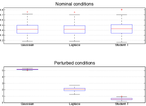
Figure 3: T-Trend Smoother: Monte Carlo simulation. Boxplot of errors obtained using Gaussian, Laplace and Student’s T Kalman smoother under nominal (top) and perturbed (bottom) conditions.

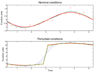
Figure 4: T-Trend Smoother: results from a Monte Carlo run under nominal (top) and perturbed (bottom) conditions using $L_{2}$ (dashed), $L_{1}$ (dashdot) and $T-Trend$ (thin line) smoother. The thick line is the true state.

7 Conclusion

We have described two new nonlinear smoothers, called T-Robust and T-Trend, which efficiently obtain the MAP estimates of the states in a state-space model with Student’s t measurement and Student’s t process noise, respectively.
The T-Robust smoother compares favorably to the $\ell_{1}$-Laplace smoother — the smoothers are comparable for most error scenarios presented, and the T-smoother has an advantage for high levels of contamination because of the re-descending influence function of the Student’s t-distribution. In addition, although it involves a non-convex objective, it is simple to implement using minor modifications to the $L_{2}$ nonlinear smoother.
The T-Trend smoother was designed for tracking signals with potential sudden changes, and has many potential applications in navigation and financial trend tracking. It was demonstrated to follow a fast jump in the state better than a smoother with a convex penalty on the innovation. Just as the T-robust smoother, it can be implemented with minor modifications to an $L_{2}$ nonlinear smoother.

8 Appendix: Full convergence theory

If $\{x^{\nu}\}$ is a sequence generated by the Gauss-Newton Algorithm 5.1 with initial point $x^{0}$ and $\varepsilon=0$, then one of the following must occur:

1. The algorithm terminates finitely at a point $x^{\nu}$ with $0\in\partial K(x^{\nu})$.

2. $\lim_{\nu\in I}\Delta_{\nu}=0$ for every subsequence $I$ for which the set $\left\{d^{\nu}\,\left|\,\nu\in I\right.\right\}$ is bounded.

3. The sequence $\|d^{\nu}\|$ diverges to $+\infty$.

Moreover, if $\bar{x}$ is any cluster point of a subsequence $I\subset{\bf Z_{+}}$ such that the subsequence $\{d^{\nu}|\nu\in I\}$ is bounded, then $0\in\partial K(\bar{x})$.

Proof: Assertions (i), (ii), and (iii) are a restatement of [6, Theorem 2.4] in our context, where the sets $D_{\nu}$ in [6, Theorem 2.4] are given by $D_{\nu}=D(x^{\nu},\eta)$. The requirement that $\rho$ be Lipschitz continuous on the set $\left\{(u)\,\left|\,\rho(u)\leq K(x^{0})\right.\right\}$ is an immediate consequence of the fact that $\rho$ is coercive its domain, so this set is compact. This completes the proof of (i), (ii), and (iii). By compactness, the matrices $H$ are uniformly continuous in $x$ on this set. Suppose that $\bar{x}$ is a cluster point of a sequence $I\subset{\bf Z_{+}}$ for which $\{d^{\nu}\}$ is bounded. Since $\bar{x}$ is a cluster point of $\{x^{\nu}\}$, we can take a convergent subsequence along which $\{d^{\nu}\}$ are still bounded, and by continuity $H^{\nu}$ converge to $\bar{H}=H(\bar{x})$. By Bolzano-Weierstrass, we can then find a subsequence $J\subset I$ and vector $\bar{d}\in{\mathbb{R}}^{Nn}$ such that $(x^{\nu},d^{\nu})\rightarrow_{J}(\bar{x},\;\bar{d})$. Fix any other point $\hat{d}\in{\mathbb{R}}^{Nn}$. By construction, we have

$$\begin{array}[]{lll}\Delta_{\nu}&=&\rho\left(F(x^{\nu})+F^{(1)}(x^{\nu})d^{\nu}\right)+\frac{1}{2}\|d^{\nu}\|_{H^{\nu}}^{2}-\rho\left(F(x^{\nu})\right)\\ &\leq&\eta\Delta^{*}(x^{\nu})\\ &\leq&\eta\left(\rho\left(F(x^{\nu})+F^{(1)}(x^{\nu})\hat{d}\right)+\frac{1}{2}\|\hat{d}\|_{H^{\nu}}^{2}-\rho\left(F(x^{\nu})\right)\right)\;.\end{array}$$

Taking the limit over $J$ gives

$$\begin{array}[]{lll}0&=&\rho\left(F(\bar{x})+F^{(1)}(\bar{x})\bar{d}\right)+\frac{1}{2}\|\bar{d}\|_{\bar{H}}^{2}-\rho\left(F(\bar{x})\right)\\ &\leq&\eta\left(\rho\left(F(\bar{x})+F^{(1)}(\bar{x})\hat{d}\right)+\frac{1}{2}\|\hat{d}\|_{\bar{H}}^{2}-\rho\left(F(\bar{x})\right)\right)\;.\end{array}$$

But $\hat{d}$ was an arbitrary point in ${\mathbb{R}}^{Nn}$, so in particular we must have $\Delta^{*}(\bar{x})=0$.

$\blacksquare$

A stronger convergence result is possible under stronger assumptions on $F$ and $F^{(1)}$, or on the sequence $H^{\nu}$. Fix $x^{0}\in{\mathbb{R}}^{Nn}$, and define

$$\Lambda=\left\{u\,\left|\,\rho(u)\leq K(x^{0})\right.\right\}\;,$$ (8.1)

where $\rho$ is as above. Note that $\Lambda$ is compact, since $\rho$ is coercive on its domain.

Corollary 8.1

Suppose that $F^{-1}(\Lambda)=\left\{x\,\left|\,F(x)\in\Lambda\right.\right\}$ is bounded, and either of the following assumptions hold:

$$0\leq\lambda_{\min}\leq\mathrm{eig}(H^{\nu})$$ (8.2)

$${\rm Null}\left(F^{(1)}(x)\right)=\{0\}\quad\forall\;x\in F^{-1}(\Lambda)\;.$$ (8.3)

If $\{x^{\nu}\}$ is a sequence generated by Algorithm 5.1 with initial point $x^{0}$ and $\varepsilon=0$, then $\{x^{\nu}\}$ and $\{d^{\nu}\}$ are bounded and either the algorithm terminates finitely at a point $x^{\nu}$ with $0\in\partial K(x^{\nu})$, or $\Delta_{\nu}\rightarrow 0$ as $\nu\rightarrow\infty$, and every cluster point $\bar{x}$ of the sequence $\{x^{\nu}\}$ satisfies $0\in\partial K(\bar{x})$.

Proof: First note that $F^{-1}(\Lambda)$ is closed since $F$ is continuous and $\Lambda$ is compact, therefore $F^{-1}(\Lambda)$ is compact. Hence $\overline{{\rm co}}\left(F^{-1}(\Lambda)\right)$ is also compact. Therefore, $F^{(1)}$ is uniformly continuous on $\overline{{\rm co}}\left(F^{-1}(\Lambda)\right)$ which implies that the hypotheses of Theorem 5.2 are satisfied, and so one of (i)-(iii) must hold. If (i) holds we are done, so we will assume that the sequence $\{x^{\nu}\}$ is infinite. Since $\{x^{\nu}\}\subset F^{-1}(\Lambda)$, this sequence is bounded. We now show that the sequence $\{d^{\nu}\}$ of search directions is also bounded.
Suppose that (8.2) holds. For any direction $d^{\nu}$, note that $d^{\nu}$ solves

$$\begin{array}[]{lll}&\displaystyle\min_{d}&\rho\left(F(x)+F^{(1)}(x)d\right)+\frac{1}{2}\|d\|_{H^{\nu}}^{2}\;.\end{array}$$

Therefore we have

$$\rho\left(F(x)+F^{(1)}(x)d^{\nu}\right)+\frac{1}{2}\|d^{\nu}\|_{H^{\nu}}^{2}\leq\rho\left(F(x)\right)$$ (8.4)

since we can achieve $\rho\left(F(x)\right)$ with $d=0$. Since $\rho\geq 0$, we must have $\{\frac{1}{2}\|d^{\nu}\|_{H^{\nu}}^{2}\}\leq\rho\left(F(x)\right)$, hence $\{\|d^{\nu}\|_{H^{\nu}}\}$ are bounded, and $d^{\nu}$ are bounded by (8.2).
Suppose instead that (8.3) holds. We claim that there exists $\kappa>0$ such that

$$\kappa\|d\|\leq\|F^{(1)}(x)d\|\quad\forall\;d\in{\mathbb{R}}^{Nn}\mbox{ and }x\in F^{-1}(\Lambda)\;.$$

Indeed, if this were not the case, then there would exist sequences $\{y^{i}\}\subset F^{-1}(\Lambda)$ and $\{d^{i}\}\subset{\mathbb{R}}^{Nn}$ such that $d^{i}\neq 0$ and

$$\|d^{i}\|/i>\|F^{(1)}(y^{i})d^{i}\|\quad\forall\;i=1,2,\dots\;.$$

The set $F^{-1}(\Lambda)$ is compact, hence there exists a subsequence $J\subset{\bf Z}_{+}$, vector $\bar{x}\in F^{-1}(\Lambda)$, and vector $\bar{d}\in{\mathbb{R}}^{Nn}$ with $\|\bar{d}\|=1$, such that $x^{\nu}\rightarrow_{J}\bar{x}$ and $d^{i}/\|d^{i}\|\rightarrow_{J}\bar{d}$. It follows from the inequality above that

$$\frac{1}{i}\geq\left\|\;F^{(1)}(x^{i})\frac{d^{i}}{\|d^{i}\|}\;\right\|\;.$$

Take the limit with respect to the subsequence $J$ we obtain $0\geq\|F^{(1)}(\bar{x})\bar{d}\|$. Thus $\bar{d}$ is in the kernel of $F^{(1)}(\bar{x})$ and $\bar{d}\neq 0$. This contradicts (8.3) and thereby proves the claim. For any direction $d^{\nu}$, (8.4) hods and $F(x)+F^{(1)}(x)d^{\nu}\in\Lambda$ since $\frac{1}{2}\|d\|_{H}^{2}\geq 0$. Since $\Lambda$ is compact, and $\{F(x^{\nu}),\;F(x^{\nu})+F^{(1)}(x^{\nu})d^{\nu}\}\subset\Lambda$ by construction, there is an $\alpha>0$ such that $\|u\|\leq\alpha$ for all $u\in\Lambda$ and for $\nu=1,2,\ldots,$

$$\kappa\|d^{\nu}\| \leq \|\;F^{(1)}(x^{\nu})d^{\nu}\;\|$$

$$\leq \|\;F(x^{\nu})+F^{(1)}(x^{\nu})d^{\nu}\;\|+\|F(x^{\nu})\|\;\leq\;2\alpha\;.$$

Hence the sequence $\{d^{\nu}\}$ of search directions is bounded.
In both cases, Theorem 5.2 tells us that $\Delta_{\nu}\rightarrow 0$ as $\nu\rightarrow\infty$. The final statement of the corollary follows immediately from the final statement of Theorem 5.2.

$\blacksquare$

References

- Aravkin [2010] A. Aravkin. Robust Methods with Applications to Kalman Smoothing and Bundle Adjustment. PhD thesis, University of Washington, Seattle, WA, June 2010.
- Aravkin et al. [2011a] A. Aravkin, B.M. Bell, J.V. Burke, and G. Pillonetto. Learning using state space kernel machines. In Proc. IFAC World Congress 2011, Milan, Italy, 2011a.
- Aravkin et al. [2011b] A. Aravkin, Bradley Bell, James Burke, and Gianluigi Pillonetto. An -Laplace robust Kalman smoother. IEEE Transactions on Automatic Control, 2011b.
- Bell et al. [2007-2011] B.M. Bell, G. Pillonetto, A. Aravkin, and J. V. Burke. Matlab®/Octave package for constrained and robust Kalman smoothing, 2007-2011. URL http://www.coin-or.org/CoinBazaar/ckbs/ckbs.xml.
- Bell et al. [2008] Bradley M. Bell, James V. Burke, and Gianluigi Pillonetto. An inequality constrained nonlinear Kalman-Bucy smoother by interior point likelihood maximization. Automatica, 2008.
- Burke [1985] J.V. Burke. Descent methods for composite nondifferentiable optimization problems. Mathematical Programming, 33:260–279, 1985.
- Chui and Chen [2009] Charles Chui and Guanrong Chen. Kalman Filtering. Springer, 2009.
- Fahrmeir et al. [1998] Ludwig Fahrmeir, Rita Kunstler, and Seminar Fur Statistik. Penalized likelihood smoothing in robust state space models. Metrika, 49:173–191, 1998.
- Farahmand et al. [2011] S. Farahmand, G.B. Giannakis, and D. Angelosante. Doubly robust smoothing of dynamical processes via outlier sparsity constraints. IEEE Transactions on Signal Processing, 59:4529–4543, 2011.
- Gelb [1974] A. Gelb. Applied Optimal Estimation. The M.I.T. Press, Cambridge, MA, 1974.
- Hampel et al. [1986] Frank R. Hampel, Elvezio M. Ronchetti, Peter J. Rousseeuw, and Werner A. Stahel. Robust Statistics: The Approach Based on Influence Functions. Wiley Series in Probability and Statistics, 1986.
- Kalman [1960] R. E. Kalman. A new approach to linear filtering and prediction problems. Transactions of the AMSE - Journal of Basic Engineering, 82(D):35–45, 1960.
- Lange et al. [1989] Kenneth L. Lange, Roderick J. A. Little, and Jeremy M. G. Taylor. Robust statistical modeling using the t distribution. Journal of the American Statistical Association, 84(408):881–896, 1989.
- Maronna et al. [2006] Ricardo A. Maronna, Douglas Martin, and Yohai. Robust Statistics. Wiley Series in Probability and Statistics. Wiley, 2006.
- Ohlsson et al. [2011] H. Ohlsson, F. Gustafsson, L. Ljung, and S. Boyd. State smoothing by sum-of-norms regularization. Automatica (to appear), 2011.
- Rochafellar [1970] R. T. Rochafellar. Convex Analysis. Princeton University Press, 1970.
- Rockafellar and Wets [1998] R.T. Rockafellar and R.J.B. Wets. Variational Analysis, volume 317. Springer, 1998.
- Schick and Mitter [1994] I.C. Schick and S.K. Mitter. Robust recursive estimation in the presence of heavy-tailed observation noise. The Annals of Statistics, 22(2):1045–1080, June 1994.
- Tibshirani [1996] R. Tibshirani. Regression shrinkage and selection via the LASSO. Journal of the Royal Statistical Society, Series B., 58, 1996.
- West and Harrison [1999] Mike West and Jeff Harrison. Bayesian Forecasting and Dynamic Models. Springer, second edition, 1999.