Renormalization of QCD₂

Abstract:

The low energy infrared scaling of the multi-color 2-dimensional quantum chromodynamics is determined in the framework of its bosonized model by using the functional renormalization group method in the local potential approximation. The model exhibits a single phase with a superuniversal effective potential.

1 Introduction

The low dimensional fermionic models as toy models provide an excellent playground to try and develop new ideas and methods in quantum field theory [1]. These models have only indirect physical meaning but they are much simpler than their 4-dimensional counterparts, and they usually show important characteristics of the original ones. For example the 2-dimensional quantum electrodynamics (QED₂) proved to be a good toy model for treating the soft mechanism of the quark confinement [2, 3]. The confining properties, the large-N_c expansion [4] or the baryon structure [5, 6] of QCD can also be studied in the 2-dimensional version of the model and then one can get even analytical results for the non-perturbative domain. One usually takes the bosonized version of these models which are local self-interacting scalar theories, and can be investigated in an easier way [7].

The phase structure of the QED₂ with many flavors was mapped out from its bosonized version and it was shown that it exhibits only a single phase [8, 9] as opposed to the single-flavor QED₂ (which is often referred to as the massive Schwinger model) [7, 3], which possesses a symmetric strong coupling ($e\gg m_{e}$) phase and the weak coupling ($e\ll m_{e}$) phase with spontaneously broken reflection symmetry separated by the critical value $(m_{e}/e)_{c}\sim 0.31$ as was shown by density matrix renormalization group (RG) technique [10] or by continuous RG method [11, 9].

The situation is a bit different in the case of the 2-dimensional quantum chromodynamics (QCD₂). The scalar model equivalent of the single flavor QCD₂ can be easily obtained, but the bosonization failed to treat the multi-flavor model. The solution of this problem was the introduction of the non-abelian bosonization [12]. However a single-flavor but multi-color investigation is possible with the usual abelian bosonization technique.

It is argued [13] that the multi-color QCD₂ possesses two phases, a weak coupling or quark phase, and a strong coupling or Bose phase. Elsewhere it is also argued [14] that the model has a single phase. This open question should be investigated in the low energy limit.

The bosonized version of the multi-flavor QED₂ contains sine-Gordon (SG) type periodic self-interaction terms. The scalar fields are coupled by a mass matrix giving a multi-component or layered sine-Gordon (LSG) model which is used to describe the vortex dynamics of magnetically coupled layered superconductors [15], where the number of flavors in QED₂ equals the number of layers of the condensed matter system [9]. The Bose form of the multi-color QCD₂ also contains SG type interactions, a mass matrix and a mixed term. The latter can be associated to the non-periodic term in the potential therefore it can be Taylor expanded giving further contributions to the mass matrix. The higher order terms are negligible since they do not modify the phase structure of the model. Then one can conclude that the difference between the bosonized versions of QED₂ and QCD₂, respectively stems from the different mass matrices. For the 2-flavors ($N_{f}=2$) QED₂ and the 2-colors ($N_{c}=2$) QCD₂ the mass matrices coincide, implying that these models are equivalent. It is quite surprising since the fermionic models are different. The difference between the bosonized models appears when $N_{f}>2$ and $N_{c}>2$. We note that the low energy multi-flavor QCD₂ with unequal masses can also be bosonized giving a so called generalized SG model [6, 16] but its investigation is out of the scope of this paper.

The phase transition of these models was obtained from the microscopic theory so far, which is formulated in the high energy/ultraviolet (UV) region. The low energy/infrared (IR) physics can be obtained by integrating out the quantum fluctuations one by one. Then one can get a low energy theory describing the quantum system at energy scales where the measurements are usually performed. The quantum fluctuations can be eliminated systematically by using the renormalization group (RG) method. The original fermionic models contain strong couplings in the high energy UV regime which disables one to perform a perturbative renormalization. The evolution is usually started from a perturbative region where the theory is almost interaction free. We also note that the RG equations should preserve the gauge symmetry [17]. However the bosonized version of the toy models, which are simple scalar models can be easily treated by the functional RG method. The low energy IR physics of the 2-dimensional one-component scalar field theories which contain periodic self-interaction term are well understood [9, 11, 18, 19].

Our goal in this article is to compare the phase structure of the multi-flavor QED₂ and the multi-color QCD₂ by using functional RG method. The bosonization is applicable for the original fermionic models at a certain parameter choice $\beta^{2}=4\pi$, which appears in the argument of the sine function. Therefore the value of the parameter $\beta$ has to be kept fixed during the RG evolution. It implies that the investigation which is confined to the local potential approximation (LPA) where $\beta$ does not evolve may give reliable evolutions. Although the Wilsonian renormalization procedure is very powerful in LPA [20], we choose the effective average action RG method [21, 22, 23, 19] to obtain the evolution of the models due to its more flexible usage. The RG evolution provides us the scale dependence of the couplings in the scalar model from which the scaling of the original fermionic couplings can be obtained according to the bosonization rules.

The paper is organized as follows. In Sect. 2 we introduce the bosonized versions of the investigated fermionic models and relate them to layered sine-Gordon (LSG) models. The evolution of the couplings is determined in Sect. 3. Finally, in Sect. 4 the conclusions are drawn up.

2 Bosonized models

2.1 Multi-flavor QED₂

The Lagrangian of the multi-flavor QED₂ is

$${\cal L}=-\frac{1}{4}F_{\mu\nu}F^{\mu\nu}+\sum_{i=1}^{N_{f}}\bar{\psi}_{i}\gamma^{\mu}(\partial_{\mu}-{\rm i}eA_{\mu})\psi_{i}-m_{e}\sum_{i=1}^{N_{f}}\bar{\psi}_{i}\psi_{i},$$ (1)

with $N_{f}$ Dirac fields and identical fermionic charge $e$ and mass $m_{e}$, furthermore $F_{01}=\partial_{0}A_{1}-\partial_{1}A_{0}$. One can transform the fermionic field variables $\bar{\psi}_{i},\psi_{i}$ into bosonic ones $\phi_{j}$ by the bosonization rules [24, 25, 2]

$$:\bar{\psi}_{i}\psi_{i}: \to -\frac{cm_{e}e}{\sqrt{\pi}}\cos(2\sqrt{\pi}\phi_{i}),$$

$$:\bar{\psi}_{i}\gamma_{5}\psi_{i}: \to -\frac{cm_{e}e}{\sqrt{\pi}}\sin(2\sqrt{\pi}\phi_{i}),$$

$$:\bar{\psi}_{i}\gamma_{\mu}\psi_{i}: \to \frac{1}{\sqrt{\pi}}\varepsilon_{\mu\nu}\partial^{\nu}\phi_{i},$$

$$:\bar{\psi}_{i}{\rm i}\mbox{$\partial\!\!\!/$}\psi_{i}: \to \frac{1}{2}{\cal N}_{m_{e}}(\partial_{\mu}\phi_{i})^{2},$$ (2)

where ${\cal N}_{m_{e}}$ means normal ordering with respect to the fermion mass $m_{e}$ and $c=\exp(\gamma)/2\pi$, with the Euler constant $\gamma=0.5774$. The Hamiltonian of the system in Coulomb gauge is given by

$${\cal H}=\sum_{i=1}^{N_{f}}\int_{x}\bar{\psi}_{i}(x)({\rm i}\gamma_{1}\partial_{1}+m_{e})\psi_{i}(x)-\frac{e^{2}}{4}\int_{x,y}j_{0,x}|x-y|j_{0,y},$$ (3)

with $\int_{x}=\int_{0}^{T}dx^{0}\int_{-L}^{L}dx^{1}$ and

$$j_{0,x}=:\sum_{i=1}^{N_{f}}\bar{\psi}_{i}(x)\gamma_{0}\psi_{i}(x):=\frac{1}{\sqrt{\pi}}\partial_{1}\sum_{i=1}^{N_{f}}\phi_{i}(x).$$ (4)

The resulting bosonized form of the Hamiltonian is

$${\cal H} = {\cal N}_{m_{e}}\int_{x}\biggl{[}\frac{1}{2}\sum_{i=1}^{N_{f}}\Pi^{2}_{i}(x)+\frac{1}{2}\sum_{i=1}^{N_{f}}(\partial_{1}\phi_{i}(x))^{2}+\frac{e^{2}}{2\pi}\left(\sum_{i=1}^{N_{f}}\phi_{i}(x)\right)^{2}$$ (5)

$$~{}~{}~{}~{}~{}~{}~{}~{}~{}~{}~{}~{}-cm_{e}^{2}\sum_{i=1}^{N_{f}}\cos\left(2\sqrt{\pi}\phi_{i}(x)\right)\biggr{]},$$

where $\Pi_{i}(x)$ denotes the momentum variable canonically conjugated to $\phi_{i}(x)$. In order to complete the bosonization, one has to use normal-ordering with respect to the scalar mass $\mu^{2}=e^{2}/\pi$ which modifies the coupling of the periodic term, ${\cal N}_{m_{e}}\cos(b\phi)=(\mu/m_{e})^{b^{2}/4\pi}{\cal N}_{\mu}\cos(b\phi)$. Therefore, the $N_{f}=1$ flavor bosonized QED₂ reads as

$${\cal H}_{N_{f}=1}={\cal N}_{\mu}\int_{x}\left[\frac{1}{2}\Pi^{2}(x)+\frac{1}{2}(\partial_{1}\phi(x))^{2}+\frac{1}{2}\mu^{2}\phi(x)^{2}-cm_{e}\mu\cos\left(2\sqrt{\pi}\phi(x)\right)\right],$$ (6)

which can be generalized for $N_{f}>1$ flavor using its rotated form where the mass matrix is diagonal. Let us note that the scalar mass term in (5) can be rewritten in terms of the mass matrix ${\cal{M}}_{{\mathrm{QED}}}^{2}$ defined via

$$\frac{1}{2}\Phi{{\cal M}^{2}_{{\mathrm{QED}}}}\Phi=\frac{1}{2}\frac{e^{2}}{\pi}\left(\sum_{n=1}^{N_{f}}a_{n}\phi_{n}\right)^{2},$$ (7)

where $\Phi=(\phi_{1},\phi_{2},...,\phi_{N_{f}})$ and the couplings $a_{n}$ are free real parameters of the model. In order to reproduce the mass term of (5) one has to restrict the choice to be $a_{n}=1$ for all $n$. However, based on symmetry considerations any choice with $a^{2}_{n}=1$ for all $n=1,\ldots,N_{f}$ should reproduce exactly the same phase structure since the number of zero and non-zero eigenvalues of the mass-matrix remains unchanged which was found to be decisive with respect to the phase structure of the $N_{f}$-component model [9]. It is not a surprise since in path-integral quantization a change of sign of any of the field components represents an allowed transformation of the integration variable, that in turn induces a single change of sign in the mass term and leaves the other terms of the action invariant. As a consequence, $a_{n}=(-1)^{n+1}$ is also a suitable choice which will be used in the mass term of QED₂ in this paper and leads to the mass matrix

$$({\cal M}_{\rm{QED}}^{2})_{a,b}=(-1)^{a+b}G,~{}~{}~{}~{}a,b=1,2,\ldots,N_{f}$$ (8)

with $G=e^{2}/\pi$. The QED-type mass matrix (8) exhibits a single non-vanishing mass-eigenvalue, $M^{2}_{N_{f}}=N_{f}G$ and $N_{f}-1$ vanishing eigenvalues.

2.2 Multi-color QCD₂

The Hamiltonian of the QCD₂ with a single flavor $N_{f}=1$ is

$${\cal H}=g^{2}\sum_{a,b=1}^{N_{c}}E_{a}^{b~{}2}+\sum_{a,b=1}^{N_{c}}\bar{\psi}^{a}\gamma_{1}(i\delta_{a}^{b}\partial_{1}-A_{a}^{b})\psi_{b}+m_{g}\sum_{a=1}^{N_{c}}\bar{\psi}^{a}\psi_{a}$$ (9)

in the gauge

$$A_{0}=0,~{}~{}A_{b}^{a}=0\mbox{~{}for~{}}a=b,~{}~{}E_{b}^{a}=0\mbox{~{}for~{}}a\neq b.$$ (10)

Using the Gauss law the bosonized Hamiltonian with one flavor becomes

$${\cal H} = \sum_{a}\left[\frac{1}{2}\left(\Pi_{a}^{2}+(\partial_{1}\phi_{a})^{2}\right)-\frac{cm_{g}\mu}{\pi}{\cal N}_{\mu}\cos(2\sqrt{\pi}\phi_{a})\right]$$ (11)

$$+\frac{g^{2}}{8\pi N_{c}}\sum_{a,b}(\phi_{a}-\phi_{b})^{2}+\frac{2c^{2}\mu^{2}}{\pi^{3/2}}\sum_{a,b}\frac{\sin(2\sqrt{\pi}(\phi_{a}-\phi_{b}))}{\phi_{a}-\phi_{b}},$$

where the scale $\mu$ should satisfy $\mu=c^{\prime}g$, with $c^{\prime}$ a constant, in order to take the interaction energy proportional to $g^{2}$ [13].

We determined the field configuration for the ground state of the model numerically. The static field configuration minimizing the energy was searched for by means of the conjugate gradient method as in [3]. The results showed that the constant field configuration with all components $\phi_{a}$ equal to the same constant minimizes the energy, for the cases $N_{c}=2,3$. The same trivial ground state appears when we take the polynomial piece of the potential alone. Therefore, it seems to be justified to Taylor-expand the last potential term in the Hamiltonian at $\phi_{a}-\phi_{b}=0$ and keep only the quadratic term of the expansion, so far one is interested in the behavior of the system in or close to the ground state. Then one finds

$${\cal H} = \sum_{a}\left[\frac{1}{2}\left(\Pi_{a}^{2}+(\partial_{1}\phi_{a})^{2}\right)-\frac{cc^{\prime}m_{g}g}{\pi}{\cal N}_{\mu}\cos(2\sqrt{\pi}\phi_{a})+\frac{1}{2}\sum_{b}g^{2}c_{g}(\phi_{a}-\phi_{b})^{2}\right]$$ (12)

with $c_{g}=1/4\pi N_{c}+(4cc^{\prime})^{2}/3$. Let us note, that similarly to the bosonized QED₂, the scalar mass term in (12) can be rewritten in terms of the mass matrix ${\cal{M}}_{{\mathrm{QCD}}}^{2}$ defined via

$$\frac{1}{2}\Phi{\cal M}_{\rm{QCD}}^{2}\Phi=\frac{1}{2}g^{2}c_{g}\sum_{a,b}(\phi_{a}-\phi_{b})^{2},$$ (13)

where $\Phi=(\phi_{1},\phi_{2},...,\phi_{N_{c}})$ and the summation runs from $a,b=1$ to $N_{c}$. Then one gets

$$({{\cal M}}^{2}_{{\mathrm{QCD}}})_{a,b}=(N-1)J\delta_{a,b}-J~{}~{}~{}~{}a,b=1,2,\ldots,N_{c}$$ (14)

with $J=2g^{2}c_{g}$. The QCD-type mass matrix (14) has a single zero eigenvalue and $N_{c}-1$ identical, non-vanishing eigenvalues, $M^{2}_{N_{c}}=N_{c}J$.

2.3 Relation to layered sine-Gordon models

Both models, the bosonized multi-flavor QED₂ and the multi-color QCD₂ can be considered as the specific forms of a generalized LSG model [9] which consists of two-dimensional periodic scalar fields coupled by an appropriate mass matrix whose bare Euclidean action is written as

$$S=\int_{x}\left[\frac{1}{2}(\partial_{\mu}\Phi)^{2}+\frac{1}{2}\Phi{\cal M}^{2}\Phi+y\sum_{n=1}^{N}\cos(\beta\phi_{n})\right]$$ (15)

with the $O(N)$ multiplet $\Phi=\left(\phi_{1},\dots,\phi_{N}\right)$. For the specific choice $\beta^{2}=4\pi$ with the mass matrices (8) and (14) one one recovers the bosonized version of the multi-flavor QED₂ for $N=N_{f}$ and that of the multi-color QCD₂ for $N=N_{c}$, respectively. The amplitude $y$ of the periodic piece of the potential is identical for all component fields, and it is proportional to the fermion mass ($y\sim m$), the exact relation can be determined by using normal-ordering w.r.t. the boson mass. We note that for $N=2$ the mass matrices (8) and (14) coincide, consequently, the Bose forms of the two-flavor QED₂ and the two-color QCD₂ are the same.

For later use it is worthwhile mentioning that after an appropriate $O(N)$ rotation diagonalizing the mass matrix, the LSG model with the QED-type mass matrix (8) exhibits a single massive field and $N-1$ massless ones. On the contrary, the LSG model with the QCD-type mass matrix (14) shows up a single massless field and $N-1$ massive fields of identical masses after such an $O(N)$ rotation.

3 RG approach for multi-component models

The systematic removal of the quantum fluctuations can be performed by the evolution equation for the effective action [21, 22, 23, 19]

$$k\partial_{k}\Gamma_{k}=\frac{1}{2}{\mathrm{Tr}}\frac{k\partial_{k}R_{k}}{\Gamma^{(2)}_{k}+R_{k}},$$ (16)

where $\Gamma^{(2)}_{k}$ refers to the second functional derivative matrix of the effective action and the trace Tr stands for the integration over all momenta. The scale $k$ starts from a large UV value $\Lambda$ (which is typically set to $\infty$ during the calculations) and goes to zero. $R_{k}$ plays the role of the IR regulator function. For the suppression of the high-frequency modes one can choose the power-law type regulator

$$R_{k}=p^{2}\left(\frac{k^{2}}{p^{2}}\right)^{b}$$ (17)

with the parameter $b\geq 1$. Here we choose $b=1$, which corresponds to the Callan-Symanzik RG scheme [23]. It is easy to see, that in $d=2$ the chosen CS scheme is free of UV divergences and ultralocal, furthermore the evolution equations take a rather simple form. We note that in $d=2$ the choices $b=1$ and $b=\infty$ coincide [26, 27] in the LPA. The latter case corresponds to the sharp cutoff limit, which makes the functional form of the CS and the sharp cutoff (or Wegner-Houghton type) evolution equations similar. The effective action is expanded in powers of the derivative of the field,

$$\Gamma_{k}[\Phi]=\int_{x}\left[V_{k}[\Phi]+Z_{k}[\Phi](\partial_{\mu}\Phi)^{2}+{\cal O}(\partial_{\mu}^{4})\right],$$ (18)

with $V_{k}[\Phi]$ the potential and $Z_{k}[\Phi]$ the wave-function renormalization. The latter provides evolution to the parameter $\beta$, even in the case of field-independent wave-function renormalization $Z_{k}[\Phi]\equiv z_{k}$, where $\beta^{2}=1/z$ [19]. The bosonization gives a constraint to the parameter $\beta^{2}=4\pi$. The running of $Z_{k}[\Phi]$ influences the evolution significantly in the vicinity of the Coleman point at $\beta^{2}=8\pi$ [19, 28] but gives slight modifications around $\beta^{2}=4\pi$ [11], therefore it is not supposed to affect the phase structure of the model. Thus we do not go beyond the LPA, and set $Z_{k}[\Phi]=1$. One can derive the evolution equation

$$(2+k\,\partial_{k})\,\,\tilde{V}_{k}({\Phi})=-\frac{1}{4\pi}\ln\left[{{\mathrm{det}}}\left(\delta_{ij}+\tilde{V}_{k}^{ij}({\Phi})\right)\right],$$ (19)

with ${\tilde{V}}_{k}^{ij}=\partial_{\phi_{i}}\partial_{\phi_{j}}{\tilde{V}}_{k}$ for the dimensionless potential ${\tilde{V}_{k}}=k^{-2}V_{k}$, where $\Phi$ stands for homogeneous field configurations. We make the general ansatz

$${\tilde{V}}_{k}({\Phi})=\frac{1}{2}{\Phi}{{{\tilde{\cal M}}}}^{2}(k){\Phi}+{\tilde{y}}(k)\sum_{n=1}^{N}\,\cos(\beta\,\phi_{n})$$ (20)

for the dimensionless potential of the LSG type models under discussion, where $\tilde{y}(k)=k^{-2}y(k)$. Inserting the ansatz (20) into Eq. (19), the right-hand side becomes periodic, while the left-hand side contains both periodic and non-periodic parts [29, 30, 31, 9]. The non-periodic part contains only mass terms, so that we obtain a RG flow equation for the dimensionless mass matrix

$$\left(2+k\partial_{k}\right){{{\tilde{\cal M}}}}^{2}(k)=0,$$ (21)

giving the scaling

$$\tilde{J}_{k}=k^{-2}J,~{}~{}\mbox{and}~{}~{}\tilde{G}_{k}=k^{-2}G,$$ (22)

which corresponds to the scaling according to the canonical dimensions, since in the LPA the anomalous dimension is zero. One can conclude that the dimensionful couplings $J$, $G$ remain constant during the blocking.

The RG flow avoids the singularities if we handle the evolution without any truncations [21]. We note however that one should usually use some approximations or expansions in the RG equations in order to solve them. The bosonized QCD₂ contains a single Fourier mode, however the RG equations generate the higher harmonics. Restricting ourselves to follow the evolution of the fundamental mode only may induce a strong truncation, implying that we should face the problem of poles of the evolution equation in Eq. (19). The proper choice of the IR regulator function may drive the evolution to reach the pole only in the $k\to 0$ limit. This seems to be true even in the case of the sharp cutoff scheme, where one can draw up the quantum cenzorship conjecture [32, 33]. However the poles – unless they appear as artifacts of the approximations and truncations, – have a great physical importance, because their existence can signal the spontaneously broken phase of the model [21, 34]. In the symmetry broken phase of a single component scalar field the dynamical Maxwell cut makes the effective potential superuniversal, namely

$$\tilde{V}_{k=0}[\Phi]=-\frac{1}{2}\Phi^{2}.$$ (23)

3.1 UV scaling

The correct UV scaling can be obtained if we improve the results of the linearized approximation by taking into account corrections of the order ${\cal O}(\tilde{J})$ for the QCD₂ type and those of ${\cal O}(\tilde{G})$ for the QED₂ type case [29, 15, 9, 30]. This is achieved by linearizing the RG equation in the periodic piece of the blocked potential,

$$(2+k\partial_{k})\tilde{V}_{k}=-\frac{1}{4\pi}\,\,\frac{F_{1}(\tilde{V}_{k})}{C}+{\cal O}(\tilde{V}_{k}^{2}),$$ (24)

where $C$ and $F_{1}(\tilde{U}_{k})$ stand for the constant and linear pieces of the determinant

$$\det[\delta_{ij}+{\tilde{V}}^{ij}_{k}]=C+F_{1}(\tilde{V}_{k})+{\cal O}(\tilde{V}_{k}^{2}).$$ (25)

The UV scaling law for the QCD₂ type LSG model for $N$ colors is

$$\tilde{y}(k)=\tilde{y}(\Lambda)\left(\frac{k}{\Lambda}\right)^{\frac{\beta^{2}}{N4\pi}-2}\left(\frac{k^{2}+NJ}{\Lambda^{2}+NJ}\right)^{\frac{(N-1)\beta^{2}}{N8\pi}}$$ (26)

with the initial value $\tilde{y}(\Lambda)$ at the UV cutoff $k=\Lambda$. From the extrapolation of the UV scaling law (26) towards the IR scales we can read off the critical value $\beta^{2}_{c}(N)=8\pi N$. The coupling $\tilde{y}$ is irrelevant for $\beta^{2}>\beta^{2}_{c}(N)$ and relevant for $\beta^{2}<\beta^{2}_{c}(N)$. The critical frequency and the corresponding critical temperature

$$T^{(N)}_{\rm{QCD}}=\frac{2\pi}{\beta_{c}^{2}(N)}=T^{\star}_{\rm{KTB}}\frac{1}{N}$$ (27)

separating the two phases of the model coincide with the general expressions obtained previously for the rotated LSG model in Refs. [29, 31, 30, 9].

Similar consideration can be done for the QED₂ type LSG model [29, 15, 9, 8] and the solution of Eq. (24) for the couplings in case of $N$ flavors is given as

$$\tilde{y}(k)=\tilde{y}(\Lambda)\left(\frac{k}{\Lambda}\right)^{\frac{(N-1)\beta^{2}}{N4\pi}-2}\left(\frac{k^{2}+NG}{\Lambda^{2}+NG}\right)^{\frac{\beta^{2}}{N8\pi}}.$$ (28)

The critical frequency and the corresponding critical temperature which separates the two phases of the model can be read off directly,

$$\beta^{2}_{c}(N)=\frac{8\pi N}{N-1},~{}\to~{}T^{(N)}_{\rm{QED}}=\frac{2\pi}{\beta_{c}^{2}(N)}=T^{\star}_{\rm{KTB}}\frac{N-1}{N}.$$ (29)

For $N=1$ layer the LSG model with magnetic type coupling reduces to the massive 2D-SG model where the periodicity is broken explicitly. Therefore, for sufficiently small bare coupling $\tilde{y}(\Lambda)$, there exists only a single phase [29, 30, 15, 9] in the $N=1$ layer model, i.e., the coupling $\tilde{y}(k)$ is relevant (increasing) in the IR limit ($k\to 0$) irrespectively of $\beta^{2}$. For $N\to\infty$ the magnetically coupled LSG behaves like a massless 2D-SG model with the critical frequency $\beta_{c}^{2}=8\pi$ [8]. Both the dependencies in Eqs. (27) and (29) of the critical frequencies $\beta_{c}$ on the number of layers $N$ indicate that QED₂ and QCD₂ with any number of flavors and colors, respectively belong to the symmetry broken phase of the corresponding LSG model ($\beta^{2}=4\pi<\beta_{c}^{2}(N)$), see also Fig. 1. We shall show below that the IR scaling laws confirm this statement.

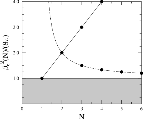
Figure 1: The critical frequency $\beta_{c}^{2}(N)$ versus the layer-number $N$ is shown for LSG models with QED₂-type (dashed line) and QCD₂-type (solid line) interlayer couplings, respectively. The critical frequencies lie outside of the shaded area, irrespectively of $N$.

The UV treatment suggests, that the phase structure of the LSG type models and the SG model is quite similar, since there is a Coleman fixed point with the critical parameter $\beta_{c}$ separating the symmetric $(\beta>\beta_{c})$ and the symmetry broken $(\beta<\beta_{c})$ phases. The Coleman point appears in the UV level, namely the couplings start to scale irrelevantly (relevantly) in the (broken) symmetric phases respectively. The inclusion of the higher harmonics modifies this picture by introducing further critical $\beta$ values [33], and may give further fixed points. However the IR behavior of the SG model results in a single Coleman point, suggesting the IR nature of the fixed point.

Occurring a pole during the RG evolution may give another signal that the bosonized multi-flavor QED₂ and multi-color QCD₂ correspond to LSG models in the symmetry broken phase. The following search for such a pole relies on the extrapolation of the UV scaling laws again. Nevertheless, the appearance of a pole would inform one on the superuniversality of the effective potential settling it as (23) with the consequence that the original multi-color QCD₂ exhibits a single phase.

As stated earlier, QED₂ for $N_{f}=2$ and QCD₂ for $N_{c}=2$ coincide. It was shown [8] that these models have a single phase. The situation changes for $N_{f}=3$ and $N_{c}=3$, respectively. Then the RG equation in Eq. (19) for 3 layers has the form

$$(2+k\partial_{k})\tilde{V}_{k} = -\frac{1}{4\pi}\log\biggl{[}(1+\tilde{V}_{k}^{11})(1+\tilde{V}_{k}^{22})(1+\tilde{V}_{k}^{33})+\tilde{V}_{k}^{12}\tilde{V}_{k}^{23}\tilde{V}_{k}^{31}+\tilde{V}_{k}^{13}\tilde{V}_{k}^{21}\tilde{V}_{k}^{32}$$ (30)

$$-\tilde{V}_{k}^{13}(1+\tilde{V}_{k}^{22})\tilde{V}_{k}^{31}-\tilde{V}_{k}^{12}\tilde{V}_{k}^{21}(1+\tilde{V}_{k}^{33})-(1+\tilde{V}_{k}^{11})\tilde{V}_{k}^{23}\tilde{V}_{k}^{32}\biggr{]}.$$

For the 3-flavor QED₂ the potential for the corresponding scalar model is

$$\tilde{V}_{k}=\frac{1}{2}\tilde{G}(\phi_{1}-\phi_{2}+\phi_{3})^{2}+\tilde{y}\bigl{[}\cos(\beta\phi_{1})+\cos(\beta\phi_{2})+\cos(\beta\phi_{3})\bigr{]}$$ (31)

with $\tilde{G}>0$. Inserting this ansatz into the argument of the logarithm in the right hand side of the RG equation (30) one can see, that a pole for $\phi_{1}=\phi_{2}=\phi_{3}=0$ may appear when

$$(1-\beta^{2}\tilde{y})^{2}(1+3\tilde{G}-\beta^{2}\tilde{y})=0.$$ (32)

Due to the factor in the first bracket in the left hand side, the relevant scaling of the dimensionless coupling $\tilde{y}$ in Eq. (28) drives the flow to a pole independently of the UV initial parameters of the model. This simple treatment suggests that the model is in its symmetry broken phase, which implies that the 3-flavor QED₂ has a single phase. Thorough calculations showed the same result [9, 8].

The form of the potential for the 3-color QCD₂ is

$$\tilde{V}_{k}=\frac{1}{2}\tilde{J}[(\phi_{1}-\phi_{2})^{2}+(\phi_{2}-\phi_{3})^{2}+(\phi_{3}-\phi_{1})^{2}]+\tilde{y}[\cos(\beta\phi_{1})+\cos(\beta\phi_{2})+\cos(\beta\phi_{3})]$$ (33)

with $\tilde{J}>0$. The argument of the logarithm in Eq. (30) is now

$$(1-\beta^{2}\tilde{y})(1+3\tilde{J}-\beta^{2}\tilde{y})^{2}=0,$$ (34)

which also gives a pole due to the first bracket in the left hand side if we consider the relevant scaling of the coupling $\tilde{y}$ according to Eq. (26). Similarly to the result obtained for the 3-flavor QED₂ the model seems to be in the symmetry broken phase giving again a single phase for the original 3-color QCD₂. Below we shall show that our expectation of a single phase for 3-color QCD₂ is justified by the IR scaling laws.

3.2 IR scaling

A more reliable information on the phase structure of the multi-color QCD₂ should be deduced from the IR scaling laws of the corresponding LSG type model. The proper treatment of the problem requires to find the solution of the rather complicated partial differential equation (19). Instead of treating that task in its full complexity, we shall invent the following strategy. First we perform an $O(N)$ rotation ${\cal R}$ which diagonalizes the symmetric mass matrix by the rotated field variables $\alpha_{i}={\cal R}_{ij}\phi_{j}$. Due to the particular structure of the mass matrix ${\cal M}^{2}_{QCD}$, it exhibits a single zero eigenvalue and $N-1$ identical eigenvalues $N{\tilde{J}}$. Further on, we assume that the mass gap suppresses large amplitude quantum fluctuations of the massive field components and, therefore the potential can be Taylor-expanded in the massive field components at their vanishing value. Then the massive fields appear in the lowest order as free fields and decouple from the massless field component and can easily be integrated out. In this manner the problem becomes amenable for the numerical treatment. Such an approach has been successfully applied to LSG models in [31].

In particular, the rotation for $N=3$ is performed with the matrix

$${\cal R}=\begin{pmatrix}\frac{1}{\sqrt{3}}&\frac{1}{\sqrt{3}}&\frac{1}{\sqrt{3}}\\ -\frac{1}{\sqrt{2}}&0&\frac{1}{\sqrt{2}}\\ \frac{1}{\sqrt{6}}&-\frac{\sqrt{2}}{\sqrt{3}}&\frac{1}{\sqrt{6}}\\ \end{pmatrix}$$ (35)

and the effective action of the rotated model takes the form

$$\Gamma_{{\mathrm{rot}}}=\int_{x}\left[\frac{1}{2}(\partial_{\mu}\alpha_{1})^{2}+\frac{1}{2}(\partial_{\mu}\alpha_{2})^{2}+\frac{1}{2}(\partial_{\mu}\alpha_{3})^{2}+\frac{3}{2}\tilde{J}(\alpha_{2}^{2}+\alpha_{3}^{2})+V_{{\mathrm{rot}}}\right],$$ (36)

with

$$V_{{\mathrm{rot}}} = 2\tilde{y}\cos\left(\beta\frac{\alpha_{1}}{\sqrt{3}}\right)\cos\left(\beta\frac{\alpha_{2}}{\sqrt{2}}\right)\cos\left(\beta\frac{\alpha_{3}}{\sqrt{6}}\right)-2\tilde{y}\sin\left(\beta\frac{\alpha_{1}}{\sqrt{3}}\right)\cos\left(\beta\frac{\alpha_{2}}{\sqrt{2}}\right)\sin\left(\beta\frac{\alpha_{3}}{\sqrt{6}}\right)$$ (37)

$$+\tilde{y}\cos\left(\beta\frac{\alpha_{1}}{\sqrt{3}}\right)\cos\left(\beta\frac{\alpha_{2}}{\sqrt{6}}\right)^{2}-\tilde{y}\cos\left(\beta\frac{\alpha_{1}}{\sqrt{3}}\right)\sin\left(\beta\frac{\alpha_{2}}{\sqrt{6}}\right)^{2}$$

$$+\tilde{y}\sin\left(\beta\frac{\alpha_{1}}{\sqrt{3}}\right)\cos\left(\beta\frac{\alpha_{2}}{\sqrt{6}}\right)\sin\left(\beta\frac{\alpha_{2}}{\sqrt{6}}\right).$$

Now we keep the lowest-order term of the Taylor-expansion of the potential in the massive field components at $\alpha_{2}=\alpha_{3}=0$ like in [31] for the LSG model. Then the effective action reduces to

$$\Gamma^{{\mathrm{red}}}_{{\mathrm{rot}}}=\int_{x}\left[\frac{1}{2}(\partial_{\mu}\alpha_{1})^{2}+3\tilde{y}\cos\left(\beta\frac{\alpha_{1}}{\sqrt{3}}\right)\right].$$ (38)

The massive components decouple and describe free fields, and by integrating out the $N-1$ massive modes as described in Refs. [31, 9] one obtains that the IR behavior of the model is completely determined by the remaining massless component field $\alpha_{1}$ which describes a simple SG model.

The advantage of the rotation reveals itself in the reduction of the task of the low-energy QCD₂ to the determination of the IR behavior of the SG model (38). The functional RG method showed [35, 18, 19] that this SG model has two phases depending on the value of its parameter $\beta^{2}/3$. As we have shown previously in Sect. 3.1 , the multi-color QCD₂ gives values of the parameter $\beta^{2}=4\pi<\beta_{c}^{2}(N)$ for arbitrary number $N>1$ of colors, which means that the corresponding SG model is in the symmetry broken phase. Earlier calculations based on Fourier expansion [35, 36, 18, 26] showed that in the symmetry broken phase the effective potential is superuniversal with the parabolic shape (23). It happened numerically that the Fourier-expansion drove the evolution towards the pole at a non-vanishing scale. Approaching it a parabolic prepotential appeared but the Fourier-expansion became unreliable at the same time, so that the further evolution was treated at tree level [37] which always gave parabolic effective potential (23). More precise calculations, avoiding any expansion of the potential [33] now suggest, however, that there is a non-trivial IR attractive fixed point for low values of $\beta^{2}$ giving a superuniversal effective potential which deviates a little from Eq. (23), and the latter form is reached only in the limit $\beta^{2}\to 0$.

The flow of the coupling $\tilde{y}$ is determined by a computer algebraic program [27], which solves the RG equation directly, without using any ansatz for the potential. It finds the fundamental mode $\tilde{y}(k)$ by Fourier-analyzing the numerically determined potential at any scale $k$ afterwards. The polynomial suppression scheme we use here needs higher numerical accuracy as compared to the exponential scheme [21]. We set a high numerical working precision in order to handle the numerical ambiguities properly as was pointed in [33]. The IR flow of the coupling can be seen in Fig. 2.

Figure 2: The IR scaling of the dimensionless coupling $\tilde{y}$ for several initial values. The inset demonstrates the convexity of the effective action during the evolution as the scale $k$ decreases, $k/\Lambda=10^{-a}$.

The figure clearly shows that the IR value of the dimensionless coupling $\tilde{y}(0)$ is independent of its initial, microscopic value. This implies that the IR effective potential is also independent of the microscopic parameters, i.e. it is superuniversal. According to the inset of Fig. 2 the effective potential approaches the parabolic shape characterized by $1+\tilde{V}^{\prime\prime}(\Phi)=0$ in the limit $k\to 0$, but our high-precision calculation also shows that it does not reach the parabola, in accordance with the findings in [33].

The dimensionful parameter $J=g^{2}c_{g}$ is constant, therefore the fermionic coupling $g$ remains unchanged during the evolution. It gives non-vanishing coupling in the IR limit of the 3-color QCD₂. The IR behavior of the model shows that the dimensionful coupling $y$ goes to zero for $k\to 0$ driving the quark mass $m_{g}$ to zero. Therefore this scalar model is a free massive theory too as was the 3-flavor QED₂ [8], and the 3-color QCD₂ is an interacting theory of massless two-dimensional quarks.

3.3 Large $N$ case

The techniques used in the previous subsections can be easily generalized to the case of arbitrary $N$. The naive expectation that multi-color QCD₂ is in the symmetry broken phase stems from the appearance of poles if we consider the argument of the logarithm in the right hand side in Eq. (34) for $N$ colors,

$$(1-\beta^{2}\tilde{y})(1+N\tilde{J}-\beta^{2}\tilde{y})^{N-1}=0$$ (39)

in the framework of the extrapolation of the UV scaling laws. Similarly to the 3-color case, the first factor can change sign due to the relevant UV scaling of the coupling $\tilde{y}$, signaling the appearance of the pole and the symmetry broken phase. However, a more reliable conclusion can be drawn again if one considers the IR scaling for $N$-colors. In order to diagonalize the mass matrix, one performs the appropriate $O(N)$ rotation. Taylor-expanding the potential in the new massive field variables $\alpha_{i}$, $i=2\ldots N$ at their vanishing values and keeping the quadratic terms only, these become massive free fields. Integrating them out one can reduce the effective action to that of the single massless field $\alpha_{1}$,

$$\Gamma^{{\mathrm{red}}}_{{\mathrm{rot}}}=\int_{x}\left[\frac{1}{2}(\partial_{\mu}\alpha_{1})^{2}+N\tilde{y}\cos\left(\beta\frac{\alpha_{1}}{\sqrt{N}}\right)\right].$$ (40)

This is a SG model too with decreasing parameter $\beta^{\prime}=\beta/\sqrt{N}$ for increasing number $N$ of colors. The calculation for smaller values of $\beta^{\prime}$ requires extreme accuracy. We set the working precision to several hundreds during the calculations to get some reliable numerical information for the model. If the effective potential is a parabola in Eq. (23) then the IR value of the dimensionless coupling is

$$\tilde{y}=\frac{2}{\beta^{2}}.$$ (41)

If we take the parameters from Eq. (40), then this relation becomes the same. Let us note here, that the IR value (41) differs a factor of 2 of the one for which the pole occurs in Eq. (39). This is due to the circumstance that the relation (39) corresponds to the neglection of the higher-harmonics of the blocked periodic potential, whereas our numerical approach avoiding the Fourier-expansion takes automatically all higher harmonics with. In order to enlighten the deviation of our result from the Maxwell-cut induced parabolic effective potential (23) it is reasonable to plot $2-\tilde{y}\beta^{2}$ as the function of the color $N$, see Fig. 3. We succeeded to calculate it only up to $N=5$. Nevertheless the figure clearly shows that $\tilde{y}\to 2/\beta^{2}$ for $N\to\infty$.

Figure 3: The $N$ dependence of the function $2-\tilde{y}\beta^{2}$.

These results also give vanishing dimensionful coupling $y$ in the IR limit. One can have the same conclusion as was obtained in the 3-color case, namely the low energy $N$-color QCD₂ is a massless interacting theory.

4 Summary

The phase structure of the bosonized version of the multi-color QCD₂ is mapped out and it was shown, that the model possesses a single phase.

After bosonization of the original fermionic model a periodic self-interacting scalar model is obtained with a mass matrix. The more involved last self-interaction term of the Hamiltonian (11) is shown to be treatable by Taylor-expansion giving further corrections to the mass matrix, so far the system is considered in or close to the ground state. The bosonized 2-color QCD₂ coincides with the 2-flavor QED₂ which implies the similar trivial phase structures of these models. The bosonized 3-color QCD₂ and 3-flavor QED₂ are, however, different models. The bosonized 3-flavor QED₂ is known to be in the symmetry (periodicity) broken phase and represents a free massive theory. The scaling laws and the phase structure of the bosonized multi-color QCD₂ has been determined by the functional RG technique, applying the Callan-Symanzik renormalization scheme. The periodic self-interaction has been found to be UV relevant, which tries to drive the flow into a pole, signaling that the $N$-color QCD₂ is in the symmetry broken phase. The IR physics of the $N$-color QCD₂ has been also determined after diagonalizing the mass matrix and integrating out the massive fields in the free-field approximation. It was found that the bosonized multi-color QCD₂ represents effectively a SG-type model in the symmetry broken phase, characterized by a superuniversal dimensionless effective potential. In the IR limit the quantum fluctuations try to drive the system to a non-trivial saddle point what seems to be, however, never reached at finite energy scale. Nevertheless, the larger the number $N$ of colors is the closer the dimensionless effective potential is driven to the parabolic shape (23). Making use of the bosonization relations, we have concluded that the $N$-color QCD₂ is a massless interacting fermionic model.

References

- [1] E. Abdalla, M.C.B. Abdalla and K.D. Rothe, Non-perturbative Methods in Two-Dimensional Quantum Field Theory, (World Scientific, Singapore, 1991).
- [2] W. Fischler, J. Kogut, L. Susskind, Phys. Rev. D19, 1188, (1979).
- [3] Y.-C. Kao, Y.-W. Lee, Phys. Rev. D50, 1165, (1994); S. Nagy, J. Polonyi, K. Sailer, Phys. Rev. D70, 105023 (2004); M. A. Metlitski, Phys. Rev. D75, 045004 (2007).
- [4] G. t’ Hooft, Nucl. Phys. B 75, 461, (1974).
- [5] Y. Frishman, J. Sonnenschein, Phys. Rept. 223, 309 (1993); J. Ellis, Y. Frishman, M. Karliner, Phys. Lett. B566, 201 (2003); J. Ellis, Y. Frishman, JHEP 0508, 081 (2005).
- [6] H. Blas JHEP 0703, 055 (2007).
- [7] S. Coleman, R. Jackiw, L. Susskind, Annals of Physics 93, 267, (1975); H. J. Rothe, K. D. Rothe, J. A. Swieca, Phys. Rev. D19, 3020, (1979).
- [8] S. Nagy, Phys. Rev. D79, 045004, (2009).
- [9] I. Nandori, Phys. Lett. B662, 302 (2008).
- [10] T. M. R. Byrnes, P. Sriganesh, R. J. Bursill and C. J. Hamer, Nucl. Phys. B (Proc. Suppl.) 109A, 202 (2002); Phys. Rev. D66, 013002 (2002).
- [11] S. Nagy, I. Nandori, J. Polonyi, K. Sailer, Phys. Rev. D77, 025026 (2008).
- [12] E. Witten, Commun. Math. Phys. 92, 455, (1984); C. M. Naón, Phys. Rev D 31, 2035 (1985); D. Gepner, Nucl. Phys. B252, 481 (1985).
- [13] V. Baluni, Phys. Lett. B90, 407 (1980).
- [14] E. Abdalla, R. Mohayaee, A. Zadra, Int. J. Mod. Phys A12, 4539 (1997); R. Mohayaee, hep-th/9705243.
- [15] I. Nandori, K. Vad, S. Meszaros, U. D. Jentschura, S. Nagy, K. Sailer, J. Phys.: Condens. Matter 19, 496211 (2007); 19, 236226 (2007).
- [16] H. Blas, JHEP 0701, 027 (2007).
- [17] M. Reuter, C. Wetterich, Nucl. Phys. B391, 147 (1993); J. Alexandre, J. Polonyi, K. Sailer, Phys. Lett. B531, 316 (2002); T. R. Morris, Oliver J. Rosten, J. Phys. A39, 11657 (2006); S. Arnone, T. R. Morris, O. J. Rosten, Eur. Phys. J. C50, 467 (2007).
- [18] S. Nagy, I. Nandori, J. Polonyi, K. Sailer, Phys. Lett. B647, 152 (2007).
- [19] S. Nagy, I. Nandori, J. Polonyi, K. Sailer, Phys. Rev. Lett. 102 (2009).
- [20] A. Hasenfratz, P. Hasenfratz, Nucl. Phys. B 270, 687 (1986), Helv. Phys. Acta 59, 833 (1986).
- [21] J. Berges, N. Tetradis, C. Wetterich, Phys. Rept. 363, 223 (2002).
- [22] C. Wetterich, Phys. Lett. B 301, 90 (1993); T. R. Morris, Int. J. Mod. Phys. A9, 2411 (1994); D. F. Litim, J. Pawlowski, The Exact Renormalization Group, Word Sci 168 (1999); J. Polonyi, Central Eur. J. Phys. 1, 1 (2004); J. M. Pawlowski, Annals Phys. 322, 2831 (2007).
- [23] J. Alexandre, J. Polonyi, Annals Phys. 288, 37 (2001); J. Alexandre, J. Polonyi, K. Sailer, Phys. Lett. B 531, 316 (2002).
- [24] S. Coleman, Phys. Rev. D11, 2088, (1975); S. Mandelstam, Phys. Rev. D11, 3026, (1975); M. B. Halpern, Phys. Rev. D12, 1684, (1975).
- [25] S. Coleman, Annals of Physics 101, 239 (1976).
- [26] I. Nandori, S. Nagy, K. Sailer, A. Trombettoni, Phys. Rev. D80, 025008 (2009).
- [27] I. Nandori, S. Nagy, K. Sailer, A. Trombettoni, JHEP 1009, 069 (2010).
- [28] S. Nagy, K. Sailer, arXiv:1012.3007.
- [29] I. Nandori, S. Nagy, K. Sailer, U. D. Jentschura, Nucl. Phys. B 725, 467 (2005); I. Nandori, K. Sailer, Phil. Mag. 86, 2033 (2006).
- [30] I. Nandori, J. Phys. A: Math. Gen. 39, 8119 (2006).
- [31] U. D. Jentschura, I. Nandori, J. Zinn-Justin, Ann. Phys. 321, 2647 (2006).
- [32] V. Pangon, S. Nagy, J. Polonyi, K. Sailer, arXiv:0907.0144.
- [33] V. Pangon, S. Nagy, J. Polonyi, K. Sailer, Phys. Lett. B 694, 89 (2010).
- [34] D. F. Litim, Phys.Rev. D64, 105007 (2001).
- [35] I. Nandori, J. Polonyi, K. Sailer, Phys. Rev. D63, 045022 (2001); I. Nandori, U.D. Jentschura, K. Sailer, G. Soff, Phys. Rev. D69, 025004 (2004).
- [36] S. Nagy, K. Sailer, J. Polonyi, J. Phys. A 39, 8105 (2006).
- [37] J. Alexandre, V. Branchina, J. Polonyi, Phys. Lett. B445, 351 (1999); J. Polonyi, e-print: hep-th/0509078.