Phase Evolution in Spatial Dark States

Abstract

Adiabatic techniques using multi-level systems have recently been generalised from the optical case to settings in atom optics, solid state and even classical electrodynamics. The most well known example of these is the so called STIRAP process, which allows transfer of a particle between different states with large fidelity. Here we generalise and examine this process for an atomic centre-of-mass state with a non-trivial phase distribution and show that even though dark state dynamics can be achieved for the atomic density, the phase dynamics will still have to be considered as a dynamical process. In particular we show that the combination of adiabatic and non-adiabatic behaviour can be used to engineer phase superposition states.

Studying the wave nature of localised single particles allows fundamental questions of quantum mechanics to be addressed. Recently experimental progress has boosted this area and experiments that can control single particles have become available in various systems. These include neutral atoms in optical lattices Bloch:08 ; Khudaverdyan:05 ; Bakr:09 or microscopic dipole traps Yavuz:06 ; Sortais:06 , electrons in quantum dots Chan:04 and several others. One of the advantages of ultra-cold atomic systems is their purity and low-noise environment, which makes them well suited for applications in quantum metrology and information Briegel:00 ; Deutsch:00 .

Developing a robust toolbox for engineering using the laws of quantum mechanics is therefore an important challenge. Compared to classical physics, many applications require coherent evolution not to be disturbed and one common process needed is a mechanism that allows transfer of particles between different trapping sites. Tunneling is such a mechanism, however in its direct application it leads to Rabi oscillations which make controlled experiments difficult Mompart:03 . Recently a new method, termed coherent tunneling adiabatic passage (CTAP), has been suggested Eckert:04 ; Greentree:04 ; Eckert:06 ; Rab:08 , which is analogous to the three level techniques of STIRAP in optical physics Bergmann:98 . This technique allows for high fidelity transport between different trapping sites, with adiabaticity as the only requirement.

While STIRAP is a well investigated technique in optical systems Bergmann:98 , its translation into the atom optical realm offers many new and interesting degrees of freedom to be explored. Recently a number of studies have focussed on the effects of non-linear dynamics on the transfer process Rab:08 ; Graefe:06 . Here we add another degree of freedom by studying states with non-trivial phase distributions and show that the CTAP process is not robust with respect to conserving the phase and therefore the functional form of the density distribution. However, we also show that the process can still be used to control the phase of the quantum state in question. Phase engineering has become an important technique in the area of quantum computing recently and the convenience of adiabatic techniques is that if the associated energy eigenvalue is zero, one can make use of the usually much smaller geometrical phases Moller:07 ; Moller:08 ; Unanyan:99 . While this is true for optical systems, we will show that one has to be more careful in atom-optical settings.

Tunnelling of an individual vortex is an interesting problem in a number of systems, including Bose-Einstein condensates and Josephson junctions. The escape of a single vortex from a pinning potential in a Josephson junction has been investigated experimentally Wallraff:03 and recently the tunnelling of a vortex in Bose-Einstein condensate has been the subject of numerical study for double well potentials Salgueiro:09 . Salgueiro et al. found that the topological defect is preserved on tunnelling of the condensate and, in fact, can be replicated in such a way that each potential minimum has a single vortex Salgueiro:09 .

In the following we will first give a brief introduction to the CTAP idea and show that the standard approximation of a three level system is good for the density transport. We will then compare this approximation to the full integration of the Schrödinger equation for the problem and identify the problems for phase stability. Finally we will extend the work to look at systems with small non-linearities and conclude.

I Coherent Transport

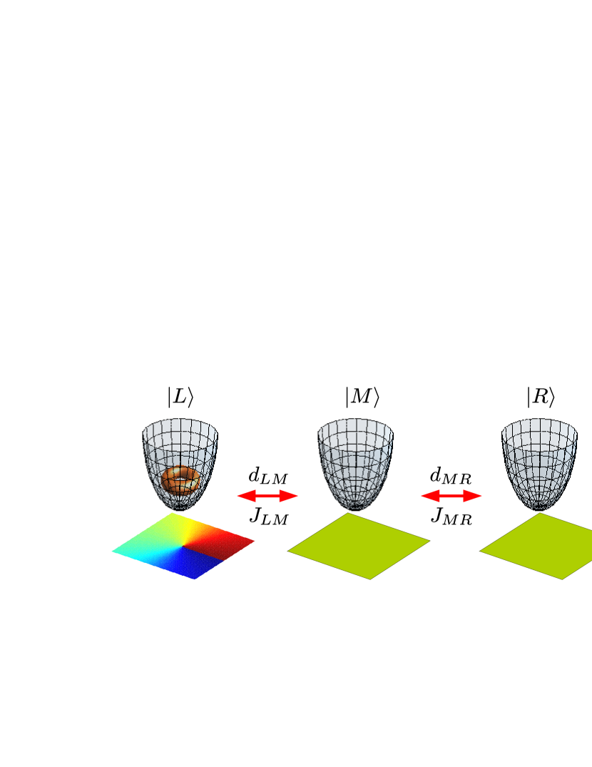
Figure 1: (Color online) Schematic setup for CTAP for an atomic state carrying one quantum of angular momentum. The atom is initially located in the trap on the left hand side and all other traps are considered empty. Tunneling only occurs between nearest neighbour traps.

The CTAP process for cold atoms considers a system of three micro-traps, between which a single particle can tunnel (see Fig. 1). The strength of the tunneling is determined by the distance and barrier height between the individual traps. If one assumes all traps to be of the same shape, i.e. have resonant energy levels, and only allows for adiabatic processes, one can write the Hamiltonian in terms of the asymptotic eigenstates of the individual traps, $|L\rangle,|M\rangle$ and $|R\rangle$, as

$$H=\begin{pmatrix}0&J_{LM}&0\\ J_{LM}&0&J_{MR}\\ 0&J_{MR}&0\end{pmatrix}\;.$$ (1)

The $J_{ij}$ are the tunneling matrix elements between neighbouring traps and we assume the tunneling between non-neighbouring traps to be negligible. The eigenstates and eigenvalues of this Hamiltonian are well known Bergmann:98 and we will focus here on the so-called dark eigenstate given by

$$|D\rangle=\cos\theta|L\rangle+\sin\theta|R\rangle\;.$$ (2)

This state only has an indirect contribution from the central trap through the mixing angle, $\tan\theta=J_{MR}/J_{LM}$, and its energy eigenvalue is given by $E_{D}=0$. If one allows for time-dependent tunneling rates, this state can be used to transfer a particle from, say, trapping site $|L\rangle$ to $|R\rangle$ with large fidelity, even in the presence of noise Eckert:04 ; Greentree:04 ; Eckert:06 . Note that during this transfer the particle has no probability to ever be in the state $|M\rangle$.

To remind the reader, let us briefly review this transfer process: the tunneling frequencies can become functions of time either through a time-dependent variation of the distance between the individual traps, through a modulation of the respective barrier heights or through a combination of both of them. Here we will assume that the trap positions change in time and, since we will assume piecewise harmonic potentials, this will also lead to a decrease in barrier height. If we therefore first decrease the distance $d_{MR}$ and, with a delay, the distance $d_{LM}$, we create the familiar counter-intuitive STIRAP timing sequence for the values of the tunneling strengths $J_{MR}$ and $J_{LM}$ (see Fig. 2 (a) and (b) and calculations below). During this process the mixing angle $\theta$ changes from $0$ to $\pi/2$ (see Fig. 2 (c)), which allows a particle initially trapped on the left hand side to be transferred to the trap on the right hand side. This is the essence of the celebrated STIRAP technique.

To calculate the tunneling frequency between two traps as a function of trap distance, let us turn to the exactly solvable model system of piecewise harmonic traps Razavy:03 ; TF , which also guarantees good approximate resonance between the levels at any point in time

$$V=\begin{cases}\frac{1}{2m}\omega^{2}\left(x+\frac{d}{2}\right)^{2}&\quad\text{for}\quad x\leq 0\\ \frac{1}{2m}\omega^{2}\left(x-\frac{d}{2}\right)^{2}&\quad\text{for}\quad x\geq 0\;.\end{cases}$$ (3)

The eigenfunctions of this potential are known to be given by parabolic cylinder functions Abramowitz

$$\psi_{1}(x) =N_{1}D_{\nu}\left[-\frac{2m\omega}{\hbar}(x+\frac{d}{2})\right] \quad\text{for}\quad x\leq 0\;,$$ (4)

$$\psi_{2}(x) =N_{2}D_{\nu}\left[\frac{2m\omega}{\hbar}(x-\frac{d}{2})\right] \quad\text{for}\quad x\geq 0\;,$$ (5)

where $N_{1}$ and $N_{2}$ are the normalisation constants. The eigenenergies are given by $E/\hbar\omega=\nu+\frac{1}{2}$ and the quantum numbers, $\nu$, are determined by requiring that the logarithmic derivatives of the two wavefunctions are equal at $x=0$

$$\left(\frac{\psi_{1}^{\prime}}{\psi_{1}}\right)_{x=0}=\left(\frac{\psi_{2}^{\prime}}{\psi_{2}}\right)_{x=0}\;.$$ (6)

By solving this condition we can exactly calculate the tunneling strength between the two traps at any time during the adiabatic process. If we then diagonalise eq. (1) we find the eigenvalues displayed in Fig. 2(d), where the dark state with the eigenvalue of zero is clearly visible. Since we assume that the whole process is carried out adiabatically, the system will be in this state at any point in time.

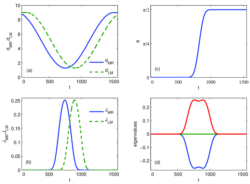
Figure 2: (Color online) (a) distance between the left-middle and the middle-right trap. (b) tunneling strength between neighbouring traps derived from the analytical model described in the text. (c) mixing angle $\theta$ and (d) time-dependent eigenvalues of the Hamiltonian (1)

I.1 Angular Momentum State

In order to write down the Hamiltonian (1) for a realistic system a number of approximations must hold. First, the eigenstates of the isolated traps have to be in close resonance, and second, the levels of the individual traps have to be chosen such that they are well isolated from all other available states in the system. The second condition can almost always be fulfiled by making the process more adiabatic and the first one translates into the simple requirement that all traps have the same trapping frequency (in case of harmonic traps). For realistic traps, however, this is problematic, as potential forces often add when they start to overlap. Several solutions have been proposed for this, including the use of time-dependent compensation potentials Eckert:06 . Here we assume that this is experimentally possible, as it allows us to isolate the physics relevant to the dynamics of the phase.

To examine the influence of the CTAP dynamics on the phase distribution of a quantum state let us first carry out a full numerical integration of the Schrödinger equation for a general system. This will at the same time function as a control mechanism for the approximations made above, in particular the fact that we neglected non-nearest neighbour coupling and treated tunneling as a one-dimensional process. For numerical simplicity, however, we will only consider a two-dimensional setup here, as this will allow us to capture the main physical processes. In scaled co-ordinates Schrödinger’s equation is therefore given by

$$i\frac{d}{dt}\psi(x,y)=\left(-\frac{1}{2}\nabla^{2}+\frac{1}{2}V(x,y)\right)\psi(x,y)\;,$$ (7)

where $V(x,y)$ is the trapping potential of the three traps in the linear configuration and which fulfils the conditions outlined above. For generality, all lengths are scaled with respect to the ground state size of the individual harmonic traps, $a_{0}=\sqrt{\hbar/m\omega}$, where $m$ is the mass of the particle and $\omega$ the trapping frequency of the individual harmonic oscillator potentials. All energies are scaled in units of the harmonic oscillator energy, $E_{0}=\hbar\omega$.

To be specific, let us choose an initial state that carries a single quantum of angular momentum and therefore has a phase distribution that increases by $2\pi$ for a closed loop around the centre of the state. This state is initially located in the trap on the left hand side. The results of the numerical integration are summarised in Fig. 3 and show surprising dynamics: while the process still leads to a 100% transfer of the probability amplitude to the trap on the right hand side (not shown), the angular momentum of the final state oscillates continuously between clockwise and counter-clockwise depending on the overall duration of the process (see upper part of the figure). Four examples of this change in phase and density associated with four different durations are shown in the lower half of the figure. In the first example (A) the system is in exactly the same state as it started out with, whereas in (B) the circulation of the flow has been reversed by the CTAP process. The plots (C) and (D) show the situation where the final state is in a superposition between clockwise and counter-clockwise rotation, which also leads to a strongly modified density distribution.

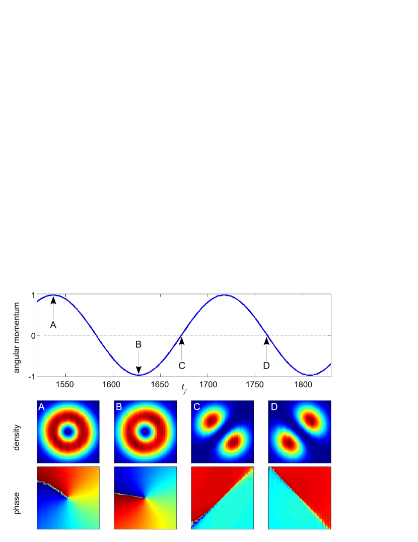
Figure 3: (Color online) Angular momentum as a function of the overall duration of the process (upper plot) and the final states in the rightmost trap at points A, B, C, and D (lower plots).

This behaviour might seem surprising at first, as angular momentum is usually thought of as a conserved quantity. However, in non-rotationally symmetric geometries this conservation law does not hold and in fact can lead to interesting dynamics for vortices in anisotropic potentials GarciaRipoll:01 ; Damski:03 ; Watanabe:07 ; PerezGarcia:07 . As in our example the particle is tunneling between rotationally symmetric potentials, it is not a priori clear where the necessary asymmetry comes from.

To gain insight into this behaviour, let us return to the three state model and consider the transport of a particle in a harmonic oscillator potential carrying one unit of angular momentum. In two dimensions its energy is given by $E_{\circ}=2\hbar\omega$ and the state is doubly degenerate, $\psi_{n_{x}n_{y}}=\psi_{10}$ and $\psi_{n_{x}n_{y}}=\psi_{01}$. We therefore have to write the most general wavefunction as the superposition

$$\psi(x,y) =\varphi_{1}(x)\varphi_{0}(y)+i\varphi_{0}(x)\varphi_{1}(y)e^{-i\theta}\;,$$ (8)

where the one-dimensional, single particle eigenfunctions of the harmonic oscillator for the ground and first excited state are given by $\varphi_{n}$. We have also allowed for a relative phase $\theta$ between the two degenerate states, however we can set this initially to zero without loss of generality.

As our traps are arranged in a linear configuration along the $y$-axis we can assume that the dynamics in the different spatial directions decouple. Tunneling therefore needs to be taken into account only for the wavefunction part in the $y$-direction and we find that the Hamiltonian can be split into one for the ground state parts of the wavefunction and one for the excited states

$$H_{0}=\begin{pmatrix}\epsilon_{0}&J_{0}^{LM}&0\\ J_{0}^{LM}&\epsilon_{0}&J_{0}^{MR}\\ 0&J_{0}^{MR}&\epsilon_{0}\end{pmatrix}\;,$$ (9)

and

$$H_{1}=\begin{pmatrix}\epsilon_{1}&J_{1}^{LM}&0\\ J_{1}^{LM}&\epsilon_{1}&J_{1}^{MR}\\ 0&J_{1}^{MR}&\epsilon_{1}\end{pmatrix}\;.$$ (10)

Unlike in the previous section, we cannot simply set the diagonal elements equal to zero as now both the ground state and first excited energies are involved. However, each of the Hamiltonians has still a dark eigenstate with the eigenvalues $\epsilon_{0}$ and $\epsilon_{1}$, respectively. If initially a single particle is in the trap on the left hand side in the state given by eq. (8), after the CTAP process, the Hamiltonians above lead to

$$\varphi_{0}^{L}(x) \longrightarrow\varphi_{0}^{R}(x)e^{-i\frac{1}{2}\omega t_{f}}$$ (11)

$$\varphi_{1}^{L}(x) \longrightarrow\varphi_{1}^{R}(x)e^{-i\frac{3}{2}\omega t_{f}}$$ (12)

$$\varphi_{0}^{L}(y) \longrightarrow\varphi_{0}^{R}(y)e^{-i\int_{0}^{t_{f}}\epsilon_{0}(t^{\prime})dt^{\prime}}$$ (13)

$$\varphi_{1}^{L}(y) \longrightarrow\varphi_{1}^{R}(y)e^{-i\int_{0}^{t_{f}}\epsilon_{1}(t^{\prime})dt^{\prime}}\;,$$ (14)

where $t_{f}$ is the overall duration of the process and the superscripts $L$ (left) and $R$ (right) refer to the traps the wavefunction is localised in. Note that although we have used scaled energy units, we reintroduce $\omega$ into the above expressions for clarity. One can immediately see that if $\epsilon_{0}$ and $\epsilon_{1}$ are not independent of time, the wavefunction acquires a relative phase between the two degenerate states that is dependent on the overall duration of the CTAP process

$$\psi(x,y;t_{f}) =\varphi_{1}^{R}(x)\varphi_{0}^{R}(y)e^{-i\left[\frac{3}{2}\omega t_{f}+\int_{0}^{t_{f}}\epsilon_{0}(t^{\prime})dt^{\prime}\right]}$$

$$+i\varphi_{0}^{R}(x)\varphi_{1}^{R}(y)e^{-i\left[\frac{1}{2}\omega t_{f}+\int_{0}^{t_{f}}\epsilon_{1}(t^{\prime})dt^{\prime}\right]}\;.$$ (15)

For easier understanding let us rewrite the above state by defining a global and a relative phase as

$$\gamma =\frac{3}{2}\omega t_{f}+\int_{0}^{t_{f}}\epsilon_{0}(t^{\prime})dt^{\prime}$$ (16)

$$\theta =-\omega t_{f}+\int_{0}^{t_{f}}[\epsilon_{0}(t^{\prime})-\epsilon_{1}(t^{\prime})]dt^{\prime}\;,$$ (17)

so that we can write the final state as

$$\psi(x,y;t_{f})=e^{-i\gamma}\left[\varphi_{1}^{R}(x)\varphi_{0}^{R}(y)+i\varphi_{0}^{R}(x)\varphi_{1}^{R}(y)e^{i\theta}\right]\;.$$ (18)

One can clearly see from this that any slight deviation in the difference between the asymptotic energy levels of the individual traps will have a significant effect on the final wavefunction. As, in particular, in realistic situations the shape of the individual potentials most likely strongly changes, one can expect to be unable to control the final form of the wavefunction. The CTAP process is therefore unstable with respect to states with non-trivial phase distributions 2D . However, as our example shows, this does not have to be a random process and in fact it can be used to engineer the phase of the wavefunction deterministically: by slightly changing the overall time of the process, one can cycle through all possible states for the fixed energy $E_{\circ}=2\hbar\omega$.

Since in our simulations the potentials are piecewise harmonic, it is not immediately clear where the change in energies comes from. Let us therefore in the following carefully examine our model and determine the influence of various other degrees of freedom. The crucial point is that during the CTAP process the energy eigenstates in the $y$-direction slightly change, since the potentials we are considering are only piecewise harmonic. By bringing them closer together, the height of the barrier between them changes, leading to a different asymptotic eigenstate. In fact, the eigenstates are very close to the parabolic cylinder functions defined above. As the first excited eigenstate is closer to the local maximum separating the traps, it will be shifted differently compared to the ground state. While the difference might only be small, the integration over a long, adiabatic time interval will lead to a large value for the integral. To demonstrate this, we show in Fig. 4 the energies for an atom in the state $\varphi_{0}(x)$ and $\varphi_{1}(x)$ during the CTAP process. It can be clearly seen that at the time of approach the energy eigenvalues slightly changes, as assumed above. In addition, we show that their difference, which is the integrand of Eq. 17, is not constant and thus gives rise to the time dependant $\theta(t_{f})$.

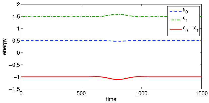
Figure 4: (Color online) Evolution of $\epsilon_{0}$ (blue dashed), $\epsilon_{1}$ (green dot-dashed) and $\epsilon_{0}-\epsilon_{1}$ (red solid) over the course of the CTAP process. Both energies are initially separated by $\omega=1$, but do not maintain this separation due to the modification of the potential as the traps move closer together.

From the above argument it follows that the effect should not only depend on the overall time of the process, but also on the minimum distance to which the traps approach each other. In Fig. 5, we show the resulting oscillations of angular momentum for a number of different values for $d_{min}$. As the minimum distance is increased, the period of the oscillations increases as well (see inset of Fig. 5), which is in accordance with the explanation given above: a larger minimum distance between the traps means that the energy levels are deviating less from the asymptotic values for perfect harmonic potentials.

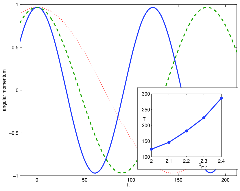
Figure 5: (Color online) Final angular momentum as a function of time for different minimum distances between the traps $d_{\text{min}}=2.0$ (full line), $d_{\text{min}}=2.2$ (dashed line) and $d_{\text{min}}=2.4$ (dotted line). The offset of the different curves has been shifted for clarity. The inset shows the increase of the period with increasing $d_{\text{min}}$.

I.2 Non-linear CTAP

Let us finally discuss the effect of a non-linearity on the evolution of the phase. The paradigm of an atomic non-linear system of well defined phase is a Bose-Einstein condensate and its dynamics can be described by the so-called Gross-Pitaevskii equation

$$H\psi(x,y)=\left(-\frac{1}{2}\nabla^{2}+V(x,y)+\frac{U}{2}|\psi|^{2}\right)\psi(x,y)\;.$$ (19)

Here $U$ is a measure for the non-linearity, which is related to the scattering strength between the atoms Pethick:08 . While the CTAP process requires resonances of the three asymptotic ground state at any time, non-linear samples break this due to the time dependence of a chemical potential, $\mu$, during the tunneling process. For large chemical potentials the whole process therefore defaults and one has to resort to different techniques for restoring the resonance during the process Rab:08 ; Nesterenko:08 . As we are only interested in the phase dynamics, we will restrict ourselves to only small non-linearities ($\mu\ll\hbar\omega$), for which about 100% transfer can still be reached.

In Fig. 6 we show the effect a small, but increasing non-linearity has on the final phase. The first thing to notice is that the oscillatory behaviour of the angular momentum does not get immediately suppressed by the non-linearity, and that the only effects are an offset and a small reduction in periodicity (not shown). We therefore speculate that the effect described in this work can also be used to create vortex superposition states in Bose-Einstein condensates in a controlled way, as long as the samples are only weakly interacting. As it is well known that vortex oscillations in an anisotropic potential can be suppressed for large enough non-linearities GarciaRipoll:01 ; Watanabe:07 , it might be interesting to study this effect in the presence of resonance restoring techniques.

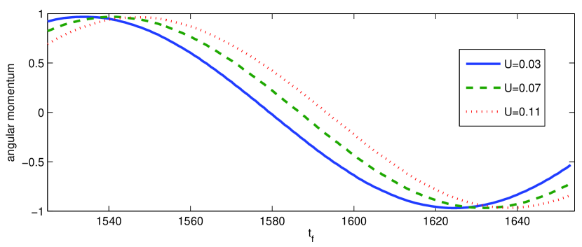
Figure 6: (Color online) Angular momentum as a function of the overall time the CTAP process takes for different non-linearities.

I.3 Conclusion

We have shown that the spatial CTAP process for atoms in microtraps does not conserve the wavefunction form for states with non-trivial phase distribution. This is due to an unavoidable small time dependence of the asymptotic eigenstates of the individual traps, which results from the overlap between them. As any currently suggested realistic systems shows large deformations due to the overlap, our work directly applies to current experimental setups.

At the same time we have shown that this instability behaves deterministically with respect to a change in the overall time of the CTAP process and can therefore be used to create well defined angular momentum superposition states. Such states can have applications in quantum information and have recently seen a surge in interest Kapale:05 ; Thanvanthri:08 . We have also shown that the presented process even survives in the presence of small non-linearities, allowing therefore to superpose vortices in Bose-Einstein condensates.