Is the minimum value of an option on variance generated by local volatility?

Abstract.

We discuss the possibility of obtaining model-free bounds on volatility derivatives, given present market data in the form of a calibrated local volatility model. A counter-example to a wide-spread conjecture is given.

keywords: local vol, Dupire’s formula; MSC: 91G99; JEL: G10.

1. Introduction

“… it has been conjectured that the minimum possible value of an option on variance is the one generated from a local volatility model fitted to the volatility surface.”; Gatheral [Gat06, page 155].

Leaving precise definitions to below, let us clarify that an option on variance refers to a derivative whose payoff is a convex function $f$ of total realized variance. Turning from convex to concave, this conjecture, if true, would also imply that that the maximum possible value of a volatility swap ($f(x)=x^{1/2}$) is the one generated from a local volatility model fitted to the volatility surface. Given the well-documented model-risk in pricing volatility swaps, such bounds are of immediate practical interest.

The mathematics of local volatility theory (à la Dupire, Derman, Kani, …) is intimately related to the following

Theorem 1 ([Gyö86]).

Assume $dY_{t}=\mu\left(t,\omega\right)dt+\sigma\left(t,\omega\right)dB_{t}$ is a multi-dimensional Itô-process where $B$ is a multi-dimensional Brownian motion, $\mu,\sigma$ are progressively measurable, bounded and $\sigma\sigma^{T}\geq\varepsilon^{2}I$ for some $\varepsilon>0$ ($\sigma^{T}$ denotes the transpose of $\sigma$). Then

(1.1) $$d\tilde{Y_{t}}=\mu_{loc}\left(t,\tilde{Y_{t}}\right)dt+\sigma_{loc}\left(t,\tilde{Y_{t}}\right)d\tilde{B}_{t},\qquad\tilde{Y}_{0}=Y_{0},$$

$$\mu_{loc}\left(t,y\right) = E\left[\mu\left(t,\omega\right)|Y_{t}=y\right],$$

$$\sigma_{loc}\left(t,y\right) = E\left[\sigma\left(t,\omega\right)\sigma^{T}\left(t,\omega\right)|Y_{t}=y\right]^{\frac{1}{2}},$$

(where the power $\frac{1}{2}$ denotes the positive square root of a positive definite matrix) has a weak solution $\tilde{Y}_{t}$ such that $\tilde{Y}_{t}\overset{law}{=}Y_{t}$ for all fixed $t$.

We will apply theorem 1 only in the simple one dimensional (resp. two dimensional in section 4 below) setting where it is well known that the solution to (1.1) is unique (cf. [Kry67] or [SV06, Capter 7]).

A generic stochastic volatility model (already written under the appropriate equivalent martingale measure and with suitable choice of numéraire) is of the form $dS=S\sigma dB$ where $\sigma=\sigma\left(t,\omega\right)$ is the (progressively measurable) instantaneous volatility process. (It will suffice for our application to assume $\sigma$ to be bounded from above and below by positive constants.) Arguing on log-price $X=\log S$ rather than $S$,

(1.2) $$dX_{t}=\sigma\left(t,\omega\right)dB_{t}-\left(\sigma^{2}\left(t,\omega\right)/2\right)dt,$$

a classical application of theorem 1 yields the following Markovian projection result: the (weak) solution to

(1.3) $$d\tilde{X}_{t} = \sigma_{loc}\left(t,\tilde{X}\right)d\tilde{B}_{t}-\left(\sigma_{loc}^{2}\left(t,\tilde{X}_{t}\right)/2\right)dt,\qquad\tilde{X}_{0}=X_{0},$$

$$(\sigma_{loc}\left(t,x\right) = E\left[\sigma^{2}\left(t,\omega\right)|X_{t}=x\right]^{\frac{1}{2}})$$

has the one-dimensional marginals of the original process $X_{t}$. Equivalently, the process $\tilde{S}=\exp\tilde{X},$

$$d{\tilde{S}}_{t}={\sigma}_{loc}(t,{\tilde{S}}_{t}){\tilde{S}}_{t}\,dB_{t},$$

known as (Dupire’s) local volatility model, gives rise to identical prices of all European call options $C\left(T,K\right)$. It easily follows that ${\sigma}_{loc}^{2}(t,{\tilde{S}})$ is given by Dupire’s formula

(1.4) $${\sigma}_{loc}^{2}(T,{\tilde{S}})|_{\tilde{S}=K}=2\frac{\partial_{T}C}{K^{2}\partial_{KK}C}.$$

Volatility derivatives are options on realized variance; that is, the payoff is given by some function $f$ of realized variance. The latter is given by

$$V_{T}:=\langle\log S\rangle_{T}=\left\langle X\right\rangle_{T}=\int_{0}^{T}\sigma^{2}(t,\omega)\,dt;$$

in the model $dS=\sigma\left(t,\omega\right)S\,dB$ and by

$$\tilde{V}_{T}:=\langle\log\tilde{S}\rangle_{T}=\langle\tilde{X}\rangle_{T}=\int_{0}^{T}\sigma_{loc}^{2}(t,\tilde{X}_{t})\,dt$$

in the corresponding local volatility model.

Common choices of $f$ are $f\left(x\right)=x$, the variance swap, $f\left(x\right)=x^{1/2}$, the volatility swap, or simply $f\left(x\right)=(x-K)^{+}$, a call-option on realized variance. See [FG05] for instance. As is well-known, see e.g. [Gat06], the pricing of a variance swap, assuming continuous dynamics of $S$ such as those specified above, is model free in the sense that it can be priced in terms of a log-contract; that is, a European option with payoff $\log S_{T}$. In particular, it follows that

$$E\left[\tilde{V}_{T}\right]=E\left[V_{T}\right].$$

Of course this can also be seen from (1.3), after exchanging ${E}$ and integration over $\left[0,T\right]$. Passing from $V_{T}$ to $f(V_{T})$ for general $f$ this is not true, and the resulting differences are known in the industry as convexity adjustment. We can now formalize the conjecture given in the first lines of the introduction.

Conjecture 1.

For any convex $f$ one has ${E}\big{[}f\big{(}{\tilde{V}_{T}}\big{)}\big{]}\leq{E}\big{[}f\big{(}{V_{T}}\big{)}\big{]}.$

Our contribution is twofold: first we discuss a simple (toy) example which provides a counterexample to the above conjecture; secondly we refine our example using a 2-dimensional Markovian projection (which may be interesting in its own right) and thus construct a perfectly sensible Markovian stochastic volatility model in which the conjectured result fails. All this narrows the class of possible dynamics for $S$ for which the conjecture can hold true and so should be a useful step towards positive answers.

2. Idea and numerical evidence

Example 2.

Consider a Black–Scholes “mixing” model $dS=S\sigma dB,S_{0}=1$ with time horizon $T=3$ in which $\sigma^{2}\left(t,\omega\right)$ is given by $\sigma_{+}^{2}(t)$ or $\sigma_{-}^{2}(t),$

$$\sigma_{+}^{2}(t):=\begin{cases}2&\mbox{if $t\in[0,1]$,}\\ 3&\mbox{if $t\in]1,2]$,}\\ 1&\mbox{if $t\in]2,3]$,}\end{cases}\quad\sigma_{-}^{2}(t):=\begin{cases}2&\mbox{if $t\in[0,1]$,}\\ 1&\mbox{if $t\in]1,2]$,}\\ 3&\mbox{if $t\in]2,3]$,}\end{cases}$$

depending on a fair coin flip $\epsilon=\pm 1$ (independent of $B$). Obviously $V=V_{3}=\int_{0}^{3}\sigma^{2}\,dt\equiv 6$ in this example, hence $E\big{[}(V-6)^{+}\big{]}=(V-6)^{+}=0$. On the other hand, the local volatility is explicitly computable (cf. the following section) and one can see from simple Monte Carlo simulations that for $\tilde{V}=\tilde{V}_{3}$

$$E\left[(\tilde{V}-6)^{+}\right]\approx 0.026>0$$

thereby (numerically) contradicting conjecture 1, with $f\left(x\right)=(x-6)^{+}$.

Our analysis of this toy model is simple enough: in section 3 below we prove that $P[\tilde{V}=6]\neq 1$. Since $E[\tilde{V}]=E[{V}]=6$ and $(x-6)^{+}$ is strictly convex at $x=6$, Jensen’s inequality then tells us that $E[(\tilde{V}-6)^{+}]>0=E\left[(V-6)^{+}\right]$.

The reader may note that an even simpler construction would be possible, i.e. one could simply leave out the interval $[0,1]$ where $\sigma_{+}^{2}$ and $\sigma_{-}^{2}$ coincide. We decided not to do so for two reasons. First, insisting on $\sigma_{+}^{2}(t)=\sigma_{-}^{2}(t)$ for $t\in[0,1]$ leads to well behaved coefficients of the SDE describing the local volatility model. Second, we will use the present setup to obtain a complete model contradicting conjecture 1 at the end of the next section.

3. Analysis of the toy example

We recall that it suffices to show that $\tilde{V}=\int_{0}^{3}{\sigma}_{loc}^{2}(t,{\tilde{X}}_{t})\,dt$ is not a.s. equal to $V\equiv 6$. The distribution of $X_{t}$ is simply the mixture of two normal distributions. More explicitly, $X_{t}=I_{\{\epsilon=+1\}}X_{t,+}+I_{\{\epsilon=-1\}}X_{t,-}$,

$$X_{t,\pm}=\int_{0}^{t}\sigma_{\pm}(s)\,dB_{s}-\tfrac{1}{2}\int_{0}^{t}\sigma_{\pm}^{2}(s)\,ds\ \ \sim\ \ N\Big{(}\tfrac{1}{2}\Sigma_{\pm}(t),\Sigma_{\pm}(t)\Big{)},$$

where $\Sigma_{\pm}(t):=\int_{0}^{t}\sigma_{\pm}^{2}(s)\,ds$. Thus ${\sigma}_{loc}^{2}(t,x)={E}[\sigma^{2}(t,\omega)|X_{t}=x]$ is given by

(3.1) $${\sigma}_{loc}^{2}(t,x)=\frac{\tfrac{\sigma_{+}^{2}(t)}{\sqrt{\Sigma_{+}(t)}}\exp\big{[}-\tfrac{(x+\Sigma_{+}(t)/2)^{2}}{2\Sigma_{+}(t)}\big{]}+\tfrac{\sigma_{-}^{2}(t)}{\sqrt{\Sigma_{-}(t)}}\exp\big{[}-\tfrac{(x+\Sigma_{-}(t)/2)^{2}}{2\Sigma_{-}(t)}\big{]}}{\tfrac{1}{\sqrt{\Sigma_{+}(t)}}\exp\big{[}-\tfrac{(x+\Sigma_{+}(t)/2)^{2}}{2\Sigma_{+}(t)}\big{]}+\tfrac{1}{\sqrt{\Sigma_{-}(t)}}\exp\big{[}-\tfrac{(x+\Sigma_{-}(t)/2)^{2}}{2\Sigma_{-}(t)}\big{]}}.$$

Since ${{\sigma_{loc}}}={{\sigma_{loc}}}(s,x)$ is bounded, measurable in $t$ and Lipschitz in $x$ (uniformly w.r.t.  $t$) and bounded away from zero it follows from [SV06, Theorem 5.1.1] that the SDE

$$d\tilde{X}_{t}=\sigma_{loc}\left(t,\tilde{X}\right)dB_{t}-\tfrac{1}{2}\sigma_{loc}^{2}\left(t,\tilde{X}_{t}\right)\,dt$$

has a unique strong solution (started from $\tilde{X}_{0}=0$, say). Since ${{\sigma_{loc}}}$ is uniformly bounded away from $0$ it follows that the process $(\tilde{X}_{t})$ has full support, i.e. for every continuous $\varphi:[0,3]\rightarrow\mathbb{R},\,\varphi(0)=0$ and every $\varepsilon>0$

$$P[\|\tilde{X}_{t}-\varphi(t)\|_{\infty;[0,T]}\leq\varepsilon]>0.$$

Indeed, there are various ways to see this: one can apply Stroock–Varadhan’s support theorem, in the form of [Pin95, Theorem 6.3] (several simplifications arise in the proof thanks to the one-dimensionality of the present problem); alternatively, one can employ localized lower heat kernel bounds (à la Fabes–Stroock [FS86]) or exploit that the Itô-map is continuous here (thanks to Doss–Sussman, see for instance [RW00, page 180]) and deduce the support statement from the full support of $B$.

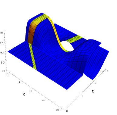
Figure 1. Time evolution of local variance $\sigma_{loc}^{2}(t,x)$ in dependence of log-moneyness. The bright strip indicates a set of paths with realized variance strictly larger than $6$.

Figure 1 illustrates the dependence of $\sigma_{loc}^{2}(t,x)$ on time $t$ and log-moneyness $x$. To gain our end of proving that $\tilde{V}\left(\omega\right)=\int_{0}^{3}{\sigma}_{loc}^{2}(t,{\tilde{X}}_{t})\,dt$ is not constantly equal $6$, we can determine a set of paths $({\tilde{X}}_{t}(\omega))$ for which $\tilde{V}$ is strictly larger than $6$. In view of Figure 1 it is natural to consider paths which are large, i.e. ${\tilde{X}}_{t}(\omega)\in[8,10]$, for $t\in]1,2-\tfrac{1}{10}]$ and small, i.e. $|{\tilde{X}}_{t}(\omega)|\leq 1$, on the interval $]2,3]$. A short mathematica-calculation reveals that $\tilde{V}\left(\omega\right)\gtrsim 6.65>6$ for each such path and according to the full-support statement the set of all such paths has positive probability, hence $\tilde{V}$ is indeed not deterministic.

Using elementary analysis it is not difficult to turn numerical evidence into rigorous mathematics. Making (3.1) explicit yields that $\sigma^{2}_{loc}(t,x)\equiv 2$ for $t\in[0,1]$ and that

(3.2) $$\sigma^{2}_{loc}(t+1,x)=\frac{\tfrac{3}{\sqrt{2+3t}}e^{-\tfrac{(2x+2+3t)^{2}}{8(2+3t)}}+\tfrac{1}{\sqrt{2+t}}e^{-\tfrac{(2x+2+t)^{2}}{8(2+t)}}}{\tfrac{1}{\sqrt{2+3t}}e^{-\tfrac{(2x+2+3t)^{2}}{8(2+3t)}}+\tfrac{1}{\sqrt{2+t}}e^{-\tfrac{(2x+2+t)^{2}}{8(2+t)}}}$$

(3.3) $$\sigma^{2}_{loc}(t+2,x)=\frac{\tfrac{1}{\sqrt{5+t}}e^{-\tfrac{(2x+5+t)^{2}}{8(5+t)}}+\tfrac{3}{\sqrt{3+3t}}e^{-\tfrac{(2x+3+3t)^{2}}{8(3+3t)}}}{\tfrac{1}{\sqrt{5+t}}e^{-\tfrac{(2x+5+t)^{2}}{8(5+t)}}+\tfrac{1}{\sqrt{3+3t}}e^{-\tfrac{(2x+3+3t)^{2}}{8(3+3t)}}}$$

for $t\in]0,1]$. We fix $\varepsilon\in]0,1]$ and observe that it is simple to see that $\lim_{x\to\infty}\sigma^{2}_{loc}(t+1,x)=3$, uniformly w.r.t. $t\in[\varepsilon,1]$, and that $\lim_{x\to 0}\sigma^{2}_{loc}(t+1,x)\geq 2$, uniformly w.r.t. $t\in]0,1]$. It follows that there exists some $\delta>0$ such that

$$\sigma^{2}_{loc}(t+1,x)\geq 3-\varepsilon\ \mbox{for $x>\tfrac{1}{\delta},t\in[\varepsilon,1]$ and }$$

$$\sigma^{2}_{loc}(t+1,x)\geq 2-\varepsilon\ \mbox{for $|x|<\delta,t\in]0,1]$.}$$

Thus we obtain

(3.4) $$\tilde{V}(\omega)=\int_{0}^{3}{\sigma}_{loc}^{2}(t,{\tilde{X}}_{t}(\omega))\,dt\geq 1\cdot 2+(1-2\varepsilon)\cdot(3-\varepsilon)+1\cdot(2-\varepsilon)$$

for every path $\tilde{X}(\omega)$ satisfying $\tilde{X}_{t}(\omega)>\tfrac{1}{\delta}$ for $t\in[1+\varepsilon,2-\varepsilon]$ and $|\tilde{X}_{t}(\omega)|<\delta$ for $t\in[2,3]$. This set of paths $\tilde{X}(\omega)$ has positive probability and the quantity on the right side of (3.4) is strictly larger than $6$ provided that $\varepsilon$ was chosen sufficiently small. Hence we find that $\tilde{V}$ is not constantly equal to $6$ as required.

For what it’s worth, the example can be modified such that volatility is adapted to the filtration of the driving Brownian motion.

The trick is to choose a random sign $\hat{\epsilon},P(\hat{\epsilon}=+1)=P(\hat{\epsilon}=-1)=\tfrac{1}{2}$ depending solely on the behavior of $(B_{t})_{0\leq t\leq 1}$ and in such a way that $S_{1}$ is independent of $\hat{\epsilon}$. For instance, if we let $m(s)$ be the unique number satisfying $P(S_{1/2}>m(s)|S_{1}=s)=P(S_{1/2}\leq m(s)|S_{1}=s)=\tfrac{1}{2}$, it is sensible to define $\hat{\epsilon}:=+1$ if $S_{1/2}>m(S_{1})$ and $\hat{\epsilon}:=-1$ otherwise.

We then leave the stock price process unchanged on $[0,1]$, i.e. we define $\hat{\sigma}^{2}(t)={\sigma}^{2}(t)=2$ and $\hat{S}_{t}=S_{t}$ for $t\in[0,1]$. On $]1,2]$ resp. $]2,3]$ we set $\hat{\sigma}^{2}(t):=2+\hat{\epsilon}$ resp. $\hat{\sigma}^{2}(t):=2-\hat{\epsilon}$ and define $\hat{S}_{t},t\in]1,3]$ as the solution of the SDE

(3.5) $$d\hat{S}_{t}=\hat{\sigma}(t)\hat{S}_{t}\,dB_{t},\ \hat{S}_{1}=S_{1}.$$

Here (3.5) depends only on $S_{1}$ and the process $(B_{t}-B_{1})_{1\leq t\leq 3}$; since both are independent of $\hat{\epsilon}$, we obtain that $(\hat{S}_{t})_{1\leq t\leq 3}$ and $(S_{t})_{1\leq t\leq 3}$ are equivalent in law. It follows that $\hat{V}=\int_{0}^{3}\hat{\sigma}^{2}(t,\omega)\,dt\equiv 6$ and since $\hat{S}_{t}$ and $S_{t}$ have the same law for each $t\in[0,3]$, they induce the same local volatility model and in particular the same (non deterministic) $\tilde{V}$.

4. Counterexample for a Markovian stochastic volatility model

Recall that $X$ denotes the log-price process of a general stochastic volatility model;

$$dX_{t}=\sigma\left(t,\omega\right)dB_{t}-\left(\sigma^{2}\left(t,\omega\right)/2\right)dt,$$

where $\sigma=\sigma\left(t,\omega\right)$ is the (progressively measurable) instantaneous volatility process. Recall also our standing assumption that $\sigma$ is bounded from above and below by positive constants. We would like to apply theorem 1 to the 2D diffusion $\left(X,V\right)$ where $dV=\sigma^{2}dt$ keeps track of the running realized variance. We can only do so after elliptic regularization. That is, we consider

$$dX_{t} = \sigma\left(t,\omega\right)dB_{t}-\left(\sigma^{2}\left(t,\omega\right)/2\right)dt,$$

$$da_{t}^{\varepsilon} = \sigma^{2}\left(t,\omega\right)dt+\varepsilon^{1/2}dZ_{t}$$

where $Z$ is a Brownian motion, independent of of the filtration generated by $B$ and $\sigma$. It follows that the following “double-local” volatility model

$$d\tilde{X}_{t}^{\varepsilon} = \sigma_{dloc}\left(t,\tilde{X}_{t}^{\varepsilon},\tilde{a}_{t}^{\varepsilon}\right)dB_{t}-\left(\sigma_{dloc}^{2}\left(t,\tilde{X}_{t}^{\varepsilon},\tilde{a}_{t}^{\varepsilon}\right)/2\right)dt,$$

$$d\tilde{a}_{t}^{\varepsilon} = \sigma_{dloc}^{2}\left(t,\tilde{X}_{t}^{\varepsilon},\tilde{a}_{t}^{\varepsilon}\right)dt+\varepsilon^{1/2}dZ_{t},$$

(with $\sigma_{dloc}^{2}\left(t,x,a\right)=E[\sigma^{2}\left(t,\omega\right)|X_{t}=x,a_{t}^{\varepsilon}=a])$ has the one-dimensional marginals of the original process $\left(X_{t},a_{t}^{\varepsilon}\right)$. That is, for all fixed $t$ and $\varepsilon$,

$$X_{t}\overset{law}{=}\tilde{X}_{t}^{\varepsilon}\text{ and }\tilde{a}_{t}^{\varepsilon}\overset{law}{=}a_{t}^{\varepsilon}\text{.}$$

Let us also note that the law of $a_{t}^{\varepsilon}$ is the law of $V_{t}=a_{t}^{0}$ convolved with a standard Gaussian of mean $0$ and variance $\varepsilon$. The log-price processes $X$ and $\tilde{X}^{\varepsilon}$ induce the same local volatility surface. To this end, just observe that $X_{t}\overset{law}{=}\tilde{X}_{t}^{\varepsilon}$ implies identical call option prices for all strikes and maturities and hence (by Dupire’s formula) the same local volatility:

$$\sigma_{loc}^{2}\left(t,x\right)=E\big{[}\sigma^{2}\big{(}t,\omega\big{)}|X_{t}=x\big{]}=E\big{[}\sigma_{dloc}^{2}\big{(}t,\tilde{X}_{t}^{\varepsilon},\tilde{a}_{t}^{\varepsilon}\big{)}|\tilde{X}_{t}^{\varepsilon}=x\big{]}.$$

Since the law of a time inhomogeneous Markov process is fully specified by its generator, it follows that the law of the local volatility process associated to $(X)$ has the same law as the local volatility process associated to $(\tilde{X}^{\varepsilon})$.

We apply this to the toy model discussed earlier. Recall that in this example, with $T=3$

$$V_{T}=\int_{0}^{T}\sigma^{2}\left(t,\omega\right)dt=6$$

whereas realized variance under the corresponding local volatilty model,

$$\tilde{V}_{T}=\int_{0}^{T}\sigma^{2}_{loc}\left(t,\tilde{X}_{t}\right)dt$$

was seen to be random (but with mean $V_{T}$, thanks to the matching variance swap prices). As a particular consequence, using Jensen

$$E\Big{(}\int_{0}^{T}\sigma_{loc}^{2}\big{(}t,\tilde{X}_{t}\big{)}dt-6\Big{)}^{+} > \Big{(}E\int_{0}^{T}\sigma_{loc}^{2}\big{(}t,\tilde{X}_{t}\big{)}dt-6\Big{)}^{+}$$

$$= \Big{(}E\int_{0}^{T}\sigma^{2}\left(t,\omega\right)dt-6\Big{)}^{+}=(V_{T}-6)^{+}=0.$$

We claim that this persists when replacing the abstract stochastic volatility model $(X)$ by $(\tilde{X}^{\varepsilon})$, the first component of a 2D Markov diffusion, for any $\varepsilon>0$. Indeed, thanks to the identical laws of the respective local volatility processes the left-hand side above does not change when replacing $(\tilde{X})$ by the local volatility process associated to $(\tilde{X}^{\varepsilon})$. On the other hand

$$E\int_{0}^{T}\sigma_{dloc}^{2}\big{(}t,\tilde{X}_{t}^{\varepsilon},\tilde{a}_{t}^{\varepsilon}\big{)}dt = E(\tilde{a}_{T}^{\varepsilon}-\varepsilon^{1/2}Z_{T})$$

$$= E\left(\tilde{a}_{T}^{\varepsilon}\right)=E\left(a_{T}^{\varepsilon}\right)$$

$$= E\big{(}V_{T}+\varepsilon^{1/2}Z_{T}\big{)}=V_{T}.$$

Thus, insisting again that the process $\tilde{X}$ is (in law) the local volatility model associated to the double local volatility model $(\tilde{X}^{\varepsilon},\tilde{a}^{\varepsilon})$ we see that

$$c=E\Big{(}\int_{0}^{T}\sigma_{loc}^{2}\big{(}t,\tilde{X}_{t}\big{)}\,dt-6\Big{)}^{+}>\Big{(}E\int_{0}^{T}\sigma_{dloc}^{2}\big{(}t,\tilde{X}_{t}^{\varepsilon},\tilde{a}_{t}^{\varepsilon}\big{)}dt-6\Big{)}^{+}=0.$$

(Observe that $c>0$ is independent of $\varepsilon$.) Using the Lipschitz property of the hockeystick function, again Gyöngy and the fact that $a^{\varepsilon}_{T}$ is normally distributed with mean $V_{T}$ and variance $\varepsilon T$ we can conclude that

$$E\Big{(}\int_{0}^{T}\sigma_{dloc}^{2}\big{(}t,\tilde{X}_{t}^{\varepsilon},\tilde{a}_{t}^{\varepsilon}\big{)}dt-6\Big{)}^{+}\!\!\! \!\!=\!\! \!E\Big{(}\int_{0}^{T}\sigma_{dloc}^{2}\big{(}t,\tilde{X}_{t}^{\varepsilon},\tilde{a}_{t}^{\varepsilon}\big{)}dt+\varepsilon^{\frac{1}{2}}Z_{T}-6-\varepsilon^{\frac{1}{2}}Z_{T}\Big{)}^{+}$$

$$\!\!\leq\!\! \!E\big{(}(\tilde{a}_{T}^{\varepsilon}-6)^{+}+|\varepsilon^{\frac{1}{2}}Z_{T}|\big{)}$$

$$\!\!=\!\! \!E(a_{T}^{\varepsilon}-6)^{+}+E|\varepsilon^{\frac{1}{2}}Z_{T}|=3\sqrt{\varepsilon T/2\pi}.$$

Now we choose $\varepsilon$ small enough such that $3\sqrt{\varepsilon T/2\pi}<c$, whence the conjecture fails to hold true in the double local volatility model for $\varepsilon>0$ small enough.

5. Conclusion

Summing up, the double-local volatility model constitutes an example of a continuous 2D Markovian stochastic volatility model, where stochastic volatility is a function of both state variables, in which conjecture 1 fails, i.e. in which the minimal possible value of a call option is not generated by a local volatility model.

References

• [BM06] D. Brigo and F. Mercurio. Interest rate models—theory and practice. Springer Finance. Springer-Verlag, Berlin, second edition, 2006. With smile, inflation and credit.
• [FS86] E. B. Fabes and D. W. Stroock. A new proof of Moser’s parabolic Harnack inequality using the old ideas of Nash. Arch. Rational Mech. Anal., 96(4):327–338, 1986.
• [FG05] P. Friz and J. Gatheral. Valuation of volatility derivatives as an inverse problem. Quant. Finance, 5(6):531–542, 2005.
• [Gat06] J. Gatheral. The volatility surface: a practitioner’s guide. WILEY, 2006.
• [Gyö86] I. Gyöngy. Mimicking the one-dimensional marginal distributions of processes having an Itô differential. Probab. Theory Relat. Fields, 71(4):501–516, 1986.
• [HL09] P. Henry-Labordère. Calibration of local stochastic volatility models to market smiles. Risk magazine, 04 Sept. 2009.
• [Kry67] N. V. Krylov. The first boundary value problem for elliptic equations of second order. Differencial nye Uravnenija, 3:315–326, 1967.
• [Lee01] R. Lee. Implied and local volatilities under stochastic volatility. International Journal of Theoretical and Applied Finance, vol 4:45–89, 2001.
• [Pin95] R. G. Pinsky. Positive harmonic functions and diffusion, volume 45 of  Cambridge Studies in Advanced Mathematics. Cambridge University Press, Cambridge, 1995.
• [Pit06] V. Piterbarg. Markovian projection method for volatility calibration. Available at SSRN: http://ssrn.com/abstract=906473, 2006.
• [RW00] L. C. G. Rogers and D. Williams. Diffusions, Markov processes, and martingales. Vol. 1. Cambridge Mathematical Library. Cambridge University Press, Cambridge, 2000. Foundations, Reprint of the second (1994) edition.
• [SV06] D. W. Stroock and S. R. Srinivasa Varadhan. Multidimensional diffusion processes. Classics in Mathematics. Springer-Verlag, Berlin, 2006. Reprint of the 1997 edition.