The dynamic dipole polarizabilities of the Li atom and the Be⁺ ion

Abstract

The dynamic dipole polarizabilities for the Li atom and the Be⁺ ion in the $2\,^{2}\!S$ and $2\,^{2}\!P$ states are calculated using the variational method with a Hylleraas basis. The present polarizabilities represent the definitive values in the non-relativistic limit. Corrections due to relativistic effects are also estimated. Analytic representations of the polarizabilities for frequency ranges encompassing the $n=3$ excitations are presented. The recommended polarizabilities for ⁷Li and ⁹Be⁺ were $164.11\pm 0.03$ $a_{0}^{3}$ and $24.489\pm 0.004$ $a_{0}^{3}$.

I Introduction

The advent of cold atom physics has lead to increased importance being given to the precise determination atomic polarizabilities and related quantities. One very important source of systematic error in the new generation of atomic frequency standards is the blackbody radiation (BBR) shift Rosenband ; Margolis ; Chwalla . The differential Stark shifts caused by the ambient electromagnetic field leads to a temperature dependent shift in the transition frequency of the two states involved in the clock transition. The dynamic polarizability is also useful in the determination of the magic wavelength in optical lattices barber ; katori ; stan ; inouye . Another area where polarization phenomena is important is in the determination of global potential surfaces for diatomic molecules leroy .

When consideration is given to all the atoms and ions commonly used in cold atom physics, the Li atom and Be⁺ ion have the advantage that they have only three electrons. This makes them accessible to calculations using correlated basis sets with the consequence that many properties of these systems can be computed to a high degree of precision. The results of these first principle calculations can serve as atomic based standards for quantities that are not amenable to precision measurement. For example, cold-atom interferometry has been used to measure the ground state polarizabilities of the Li and Na atoms miffre ; ekstrom . However the polarizability ratio, $\alpha_{d}(X)/\alpha_{d}(\text{Li})$ can be measured to a higher degree of precision than the individual polarizabilities cronin . So measurements of this ratio, in conjunction with a high precision ab-initio calculation could lead to a new level of accuracy in polarizability measurements for the atomic species most commonly used in cold-atom physics.

Calculations and measurements of Stark shifts are particularly important in atomic clock research since the BBR shift is predominantly determined by the Stark shift of the two levels involved in the clock transition. The best experimental measurements of the Stark shift have been carried out for the alkali atoms and accuracies better than 0.1$\%$ have been reported  miller ; hunter . Experimental work at this level of accuracy relies on a very precise determination of the electric field strength in the interaction region hunter ; hunter92 ; wijngaarden . High precision Hylleraas calculations of the type presented here provide an invaluable test of the experimental reliability since they provide an independent means for the calibration of electric fields stevens .

The dynamic Stark shift in oscillating electromagnetic fields is also of interest. The so-called magic wavelength, i.e. the precise wavelength at which the Stark shifts for upper and lower levels of the clock transition are the same, is an important parameter for optical lattices. The present calculation is used to estimate the magic wavelength for the Li $2\,^{2}\!S$ $\to$ $2\,^{2}\!P$ transition. The present calculations of the AC Stark shift potentially provides an atomic based standard of electromagnetic (EM) field intensity for finite frequency radiation.

There have been many calculations of the static polarizabilities of the ground and excited states of the Li atom and the Be⁺ ion tang ; yan ; yan1 ; cohen ; zhang ; johnson ; tang2 . The most precise calculations on Li and Be⁺ are the Hylleraas calculations by Tang and collaborators tang ; tang2 . The Hylleraas calculations were non-relativistic and also included finite mass effects for Li. Large scale calculations using fully correlated Hylleraas basis sets can attain a degree of precision not possible for calculations based on orbital basis sets McKDra91 ; yan1 ; yan-drake97 . There have been many calculations of the dynamic polarizability for Li merawa94 ; merawa98 ; pipin ; cohen ; chernov ; kobayashi ; muszynska ; safronova , but fewer for Be⁺ merawa98 ; muszynska . The present calculation is by far the most precise calculation of the dynamic polarizability that is based upon a solution of the non-relativistic Schrödinger equation. One particularly noteworthy treatment is the relativistic single-double all-order many body perturbation theory calculation (MBPT-SD) by Safronova et al. safronova . This calculation is fully relativistic and treats correlation effects to a high level of accuracy, although it does not achieve the same level of precision as the present Hylleraas calculation.

The present work computes the dynamic dipole polarizabilities of the Li atom and the Be⁺ ion in the $2\,^{2}\!S$, and $2\,^{2}\!P$ levels using a large variational calculation with a Hylleraas basis set. This methodology allows for the determination of the computational uncertainty related to the convergence of the basis set. Analytic representations of the dynamic polarizabilities are made so they can subsequently be computed at any frequency. Finally, the difference between the calculated and experimental binding energies is used to estimate the size of the relativistic correction to the polarizability. The final polarizabilities should be regarded as the recommended polarizabilities for comparison with experiment. All quantities given in this work are reported in atomic units except where indicated otherwise.

Table 1: Comparisons of the binding energies (in a.u.) of Li and Be⁺ in their low-lying states. The experimental valence binding energies are taken from the National Institute of Standards database ralchenko . The $J$-weighted average is used for states with $L\geq 1$. The ground-state energies for the ^∞Li⁺ and ^∞Be²⁺ ions are $-7.2799134126693059$ and $-13.6555662384235867$ a.u. respectively  drake . The ground-state energies for ⁷Li⁺ and ⁹Be²⁺ are $-7.2793215198156744$ and $-13.6547092682827917$ a.u. respectively drake . Underlining is used to indicate digits that have not converged with respect to basis set enlargement.

State	Theory		Experiment
	∞Li	7Li	6,7Li
$2\,^{2}\!S$	$-0.19814691\underline{124}$	$-0.19813041\underline{084}$	–0.198142
$2\,^{2}\!P$	$-0.13024311\underline{963}$	$-0.13023623\underline{876}$	–0.130236
$3\,^{2}\!S$	$-0.07418\underline{381350}$	$-0.07417\underline{777025}$	–0.074182
$3\,^{2}\!P$	$-0.05723\underline{769823}$	$-0.05723\underline{424577}$	–0.057236
$3\,^{2}\!D$	$-0.05561012\underline{974}$	$-0.05560578\underline{543}$	–0.055606
$4\,^{2}\!S$	$-0.037\underline{52870957}$	$-0.037\underline{52445073}$	–0.038615
$4\,^{2}\!P$	$-0.031\underline{39073613}$	$-0.031\underline{38814390}$	–0.031975
$4\,^{2}\!D$	$-0.03127\underline{588444}$	$-0.03127\underline{343938}$	–0.031274
$4\,^{2}\!F$	$-0.031253555\underline{31}$	$-0.031251112\underline{02}$	–0.031243
	∞Be+	9Be+	9Be+
$2\,^{2}\!S$	$-0.66919693\underline{847}$	$-0.66915422\underline{599}$	–0.669247
$2\,^{2}\!P$	$-0.52376705\underline{352}$	$-0.52375065\underline{365}$	–0.523769
$3\,^{2}\!S$	$-0.2672\underline{0549176}$	$-0.2671\underline{8867334}$	–0.267233
$3\,^{2}\!P$	$-0.2295\underline{6788615}$	$-0.2295\underline{5822005}$	–0.229582
$3\,^{2}\!D$	$-0.22248781\underline{972}$	$-0.22247429\underline{085}$	–0.222478
$4\,^{2}\!S$	$-0.13\underline{629487843}$	$-0.13\underline{628082370}$	–0.143152
$4\,^{2}\!P$	$-0.12\underline{222924451}$	$-0.12\underline{221999823}$	–0.128134
$4\,^{2}\!D$	$-0.12512\underline{688879}$	$-0.12511\underline{926908}$	–0.125124
$4\,^{2}\!F$	$-0.1250154671\underline{1}$	$-0.12500785\underline{769}$	–0.125008

II The structure calculations

II.1 Hamiltonian and Hylleraas coordinates

The Li atom and Be⁺ ion are four-body Coulomb systems. After separating the center of mass coordinates, the nonrelativistic Hamiltonian can be written in the form zhang_yan

$$H_{0} = -\sum_{i=1}^{3}\frac{1}{2\mu}\nabla_{i}^{2}-\frac{1}{m_{0}}\sum_{i>j\geq 1}^{3}\nabla_{i}\cdot\nabla_{j}-\sum_{i=1}^{3}\frac{Z}{r_{i}}$$ (1)

$$+ \sum_{i>j\geq 1}^{3}\frac{1}{r_{ij}}\,,$$

where $r_{ij}=|\textbf{r}_{i}-\textbf{r}_{j}|$ is the distance between electrons $i$ and $j$, $\mu=m_{0}m_{\rm e}/(m_{0}+m_{\rm e})$ is the reduced mass between the electron and the nucleus, and $Z$ is the nuclear charge. In our calculation the wave functions are expanded in terms of the explicitly correlated basis set in Hylleraas coordinates:

$$\phi({\bf{r}}_{1},{\bf{r}}_{2},{\bf{r}}_{3}) = r_{1}^{j_{1}}r_{2}^{j_{2}}r_{3}^{j_{3}}r_{12}^{j_{12}}r_{23}^{j_{23}}r_{31}^{j_{31}}e^{-\alpha r_{1}-\beta r_{2}-\gamma r_{3}}$$ (2)

$$\times \mathcal{Y}_{(\ell_{1}\ell_{2})\ell_{12},\ell_{3}}^{LM_{L}}(\hat{{\bf{r}}}_{1},\hat{{\bf{r}}}_{2},\hat{{\bf{r}}}_{3})\chi(1,2,3)\,,$$

where $\mathcal{Y}_{(\ell_{1}\ell_{2})\ell_{12},\ell_{3}}^{LM_{L}}$ is the vector-coupled product of spherical harmonics to form an eigenstate of total angular momentum $L$ and component $M_{L}$

$$\mathcal{Y}_{(\ell_{1}\ell_{2})\ell_{12},\ell_{3}}^{LM_{L}}(\hat{{\bf{r}}}_{1},\hat{{\bf{r}}}_{2},\hat{{\bf{r}}}_{3})=\!\sum_{{\rm all\,}m_{i}}\langle\ell_{1}m_{1}\ell_{2}m_{2}|\ell_{12}m_{12}\rangle$$

$$\times\langle\ell_{12}m_{12}\ell_{3}m_{3}|LM_{L}\rangle Y_{\ell_{1}m_{1}}(\hat{{\bf{r}}}_{1})Y_{\ell_{2}m_{2}}(\hat{{\bf{r}}}_{2})Y_{\ell_{3}m_{3}}(\hat{{\bf{r}}}_{3})\,,$$

(3)

and $\chi(1,2,3)$ is the three-electron spin $1/2$ wave function. The variational wave function is a linear combination of anti-symmetrized basis functions $\phi$. With some truncations to avoid potential numerical linear dependence, all terms in Eq. (2) are included such that

$$j_{1}+j_{2}+j_{3}+j_{12}+j_{23}+j_{31}\leq\Omega\,,$$ (4)

where $\Omega$ is an integer. The computational details in evaluating the necessary matrix elements of the Hamiltonian may be found in yan-drake97 . The nonlinear parameters $\alpha$, $\beta$, and $\gamma$ in Eq. (2) are optimized using Newton’s method.

The convergence for the energies and other expectation values is studied by increasing $\Omega$ progressively. The basis sets are essentially the same as two earlier Hylleraas calculations of the static polarizabilities tang ; tang2 . The maximum $\Omega$ used in the present calculations is 12. The uncertainty in the final value of any quantity is usually estimated to be equal to the size of the extrapolation from the largest explicit calculation.

Fig. 1 is a schematic diagram showing the nonrelativistic energy levels of the most important states of the Li atom. The energy level diagram for the low lying states of Be⁺ is similar.

The energies of the ground states for ^∞Li and ⁷Li were $-7.47806032391(5)$ and $-7.47745193065(5)$ a.u. respectively. The respective energies for the ^∞Be⁺ and ⁹Be⁺ ground states were $-14.3247631769(3)$ and $-14.3238634942(3)$ a.u.. Table 1 gives the binding energies of the Li atom and Be⁺ ion systems with respect to the two-electron Li⁺ and Be²⁺ cores. The Hylleraas basis was optimized to compute the $2\,^{2}\!S$ and $2\,^{2}\!P$ state polarizabilities, so some of the $n=4$ state energies have significant deviations from the experimental $n=4$ state energies. The states with significant energy differences can be regarded as pseudo-states. The uncertainties listed in Table 1 represent the uncertainties in the energy with respect to an infinite basis calculation. The actual computational uncertainty is very small and there is no computational error in any of the calculated digits listed in Table 1.

With one exception, all the finite mass binding energies are less tightly bound than experiment. The differences from experiment are most likely due to relativistic effects. The exception where experiment is less tightly bound than the finite mass calculation is the $4\,^{2}\!F$ state of Li. This exception was not investigated since the properties of this state do not enter into any of the polarizability calculations.

Figure 1: Low lying energy levels of the Li atom. The energy level diagram for Be⁺ is similar.

II.2 Polarizability definitions

The dynamic polarizability provides a measure of the reaction of an atom to an external electromagnetic field. The dynamic polarizability at real frequencies can be expressed in terms of a sum over all intermediate states, including the continuum. The dynamic dipole polarizability is expressed in terms of the dynamic scalar and tensor dipole polarizabilities, $\alpha_{1}(\omega)$ and $\alpha_{1}^{T}(\omega)$, which can be expressed in terms of the reduced matrix elements of the dipole transition operator:

$$\alpha_{1}(\omega) = \sum_{L_{a}}\alpha_{1}(L_{a},\omega)\,,$$ (5)

$$\alpha_{1}^{T}(\omega) = \sum_{L_{a}}W(L,L_{a})\alpha_{1}(L_{a},\omega)\,,$$ (6)

where

$$\alpha_{1}(L_{a},\omega)=\frac{8\pi}{9(2L+1)}\sum_{n}\frac{\Delta E_{0n}\big{|}\langle n_{0}L\|T_{1}\|nL_{a}\rangle\big{|}^{2}}{\Delta E_{0n}^{2}-\omega^{2}}\,,$$ (7)

with $T_{1}=\sum_{i=0}^{3}q_{i}R_{i}Y_{10}({\bf{\hat{R}}}_{i})$ being the dipole transition operator, and

$$W(L,L_{a}) = (-1)^{L+L_{a}}\sqrt{\frac{30(2L+1)L(2L-1)}{(2L+3)(L+1)}}$$ (8)

$$\times \left\{\begin{matrix}1&1&2\\ L&L&L_{a}\\ \end{matrix}\right\}\,.$$

In the above, $|n_{0}L\rangle$ is the initial state with principal quantum number $n_{0}$, angular momentum quantum number $L$, and energy $E_{0}$. The $n$th intermediate eigenfunction $|nL_{a}\rangle$, with principal quantum number $n$ and angular momentum quantum number $L_{a}$, has an energy $E_{n}$. The transition energy is $\Delta E_{0n}=E_{n}-E_{0}$. The $q_{i}$ are the charges of the respective particles and ${\bf R}_{i}$ are defined in Ref. zhang_yan . In particular, for the case of $L=0$,

$$\alpha_{1}(\omega) = \alpha_{1}(P,\omega)\,,$$ (9)

$$\alpha_{1}^{T}(\omega) = 0\,;$$ (10)

for $L=1$,

$$\alpha_{1}(\omega)\! = \!\alpha_{1}(S,\omega)+\alpha_{1}(P,\omega)+\alpha_{1}(D,\omega)\,,$$ (11)

$$\alpha_{1}^{T}(\omega)\! = \!-\alpha_{1}(S,\omega)+\frac{1}{2}\alpha_{1}(P,\omega)-\frac{1}{10}\alpha_{1}(D,\omega).$$ (12)

In Eqs. (11) and (12), $\alpha_{1}(P,\omega)$ is the contribution from the even-parity configuration $(pp^{\prime})P$. The scalar and tensor polarizabilities can be easily related to the polarizabilities of the magnetic sub-levels, $\alpha_{1,M}(\omega)$,

$$\alpha_{1,0}(\omega) = \alpha_{1}(\omega)-2\alpha_{1}^{T}(\omega)$$

$$\alpha_{1,\pm 1}(\omega) = \alpha_{1}(\omega)+\alpha_{1}^{T}(\omega)\ .$$ (13)

III The dynamic polarizability for the ^∞Li atom and the ^∞Be⁺ ion

III.1 Ground state dynamic polarizabilities

Figure 2: Dynamic dipole polarizability, $\alpha_{1}(\omega)$, of the Li atom in the ground state. The singularities in the polarizability at the $2\,^{2}\!S\rightarrow n\,^{2}\!P$ frequencies are marked.

Fig. 2 shows the dynamic dipole polarizability of the lithium ground state as a function of photon energy. The chief errors in the dynamic polarizability are related to the convergence of the $n\,^{2}\!P$ excited state energies. The largest calculation used a basis with dimensions $(N_{s},N_{p})=(6412,5761)$. The difference between the $\alpha_{1}(\omega)$ and polarizability computed with a $(N_{s},N_{p})=(4172,3543)$ basis would be barely discernible in Fig. 2. The convergence of $\alpha_{1}(\omega)$ is best at photon energies far from the discrete excitation energies of the $n\,^{2}\!P$ excitations. The polarizability is very susceptible to small changes in the physical energies at photon energies close to the $n\,^{2}\!P$ excitation energies.

Table 2: The dynamic dipole polarizabilities, $\alpha_{1}(\omega)$ (in a.u.), for the Li ground state. The results of the fourth column include relativistic corrections. The numbers in brackets for the second and third columns are the uncertainties in the last digits arising from incomplete convergence of the basis set. The uncertainties in the recommended (Rec.) values reflect additional uncertainties related to the relativistic correction.

$\omega$	Hylleraas			MBPT-SD safronova	TDGI	CI-Hylleraas	Model
	∞Li	7Li	Rec. 7Li		merawa94 ; merawa98	pipin	Potential cohen
0.00000	164.112(1)	164.161(1)	164.11(3)		163.6	164.1	164.14
0.00500	164.996(1)	165.045(1)	165.00(3)		164.5	165.0	165.03
0.01000	167.707(1)	167.758(1)	167.71(3)		167.2	167.7	167.74
0.02000	179.517(1)	179.574(1)	179.52(3)		178.9	179.5	179.55
0.02931	201.242(2)	201.313(1)	201.24(3)	201.0(7)
0.03000	203.438(1)	203.512(1)	203.44(3)		202.6	203.4	203.47
0.03420	219.221(1)	219.307(1)	219.22(4)	219.0(8)
0.04000	250.265(1)	250.376(1)	250.26(4)		248.8	250.3	250.29
0.04624	304.278(1)	304.441(1)	304.26(5)	304.0(8)
0.05000	356.077(1)	356.300(1)	356.05(6)		355.2	356.1	356.60
0.05699	550.259(1)	550.790(1)	550.18(9)	549.7(1.1)
0.06000	741.165(2)	742.126(1)	741.00(12)		729.2		740.73
0.06507	1984.577(1)	1991.488(1)	1983.11(31)	1983(3)
0.07000	–2581.603(2)	–2569.994(2)	–2584.54(40)		–2895.3
0.07592	–645.478(2)	–644.749(1)	–645.70(10)	–645.9(1.3)
0.08000	–415.067(1)	–414.763(1)	–415.17(7)		–427.1
0.09000	–211.518(2)	–211.439(1)	–211.55(3)		–216.5
0.09110	–199.941(1)	–199.868(1)	–199.97(3)	–200.1(0.8)
0.10000	–135.872(2)	–135.838(1)	–135.89(3)		–0.819
0.11388	–86.266(1)	–86.249(1)	–86.27(2)	–86.4(0.8)
0.15183	–38.210(9)	–38.204(9)	–38.22(1)	–38.4(1.1)
0.16000	–31.08(5)	–31.06(5)	–31.08(6)

The uncertainties in the dynamic dipole polarizabilities of the Li ground state as well as the polarizabilities themselves are listed in Table 2. All of the values listed are accurate to about $\pm 1$ in the fifth digit for $\omega\leq 0.11388$ a.u.. Some of the alternate calculations of the $\alpha_{1}(\omega)$ polarizabilities safronova ; merawa94 ; merawa98 ; pipin ; cohen are listed in Table 2. Dynamic polarizabilities from some less accurate calculations chernov ; kobayashi ; muszynska have not been tabulated.

One feature of Table 2 is the excellent agreement with the MBPT-SD calculation of Safronova et al. safronova . The MBPT-SD calculation and the present Hylleraas calculation are in perfect agreement when the MBPT-SD theoretical uncertainty is taken into consideration. While the MBPT-SD calculation is fully relativistic, its treatment of electron correlation is less exact than the present calculation. The MBPT-SD calculation also gives no consideration of finite mass effects. Relativistic effects would tend to decrease $\alpha_{1}(\omega)$ at low $\omega$, and the MBPT-SD calculation gives slightly smaller $\alpha_{1}(\omega)$ at low $\omega$.

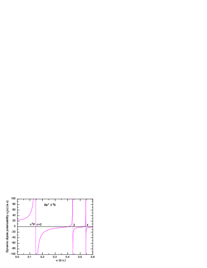
Figure 3: The dynamic dipole polarizability, $\alpha_{1}(\omega)$ for the ground state of the Be⁺ ion. The singularities in the polarizability at the $2\,^{2}\!S\rightarrow n\,^{2}\!P$ frequencies are marked.

The older CI-Hylleraas calculation of values of Pipin and Bishop pipin compares excellently with the present more modern calculation. All digits in $\alpha_{1}(\omega)$ from the CI-Hylleraas calculation are in perfect agreement with the present Hylleraas calculation. The model potential polarizabilities of Cohen and Themelis cohen are also very close to the present dynamic polarizability. The Cohen-Themelis potential was constructed using a Rydberg-Klein-Rees (RKR) inversion method. The Time-Dependent-Gauge-Invariant (TDGI) polarizabilities of Mérawa et al merawa94 ; merawa98 are only accurate to 0.5$\%$ or larger. The moderate accuracy of TDGI calculations has also been noted in calculations of the static polarizabilities tang .

The static polarizabilities for Be⁺ in the infinite mass approximation have been presented recently tang2 . The present calculation represents an extension of this earlier calculation since finite mass effects are now included. The dynamic dipole polarizabilities listed in Table 3 includes transition frequencies that extend well into the ultraviolet region. The most accurate of the few alternate calculations should be the CI-Hylleraas calculation of Muszynska et al muszynska . However, it gives an $\alpha_{1}(\omega)$ that is about 1$\%$ smaller than the present polarizability. Space limitations precluded tabulation of the TDGI polarizability merawa98 . The TDGI polarizability was of only moderate accuracy with errors of about $2\%$ for $\omega\leq 0.6$ a.u.. The uncertainty in the present polarizability is about 10^-4 a.u. for photon energies lower than 0.40 a.u., but has increased to 10^-2 a.u. at $\omega=0.50$ a.u..

Table 3: Dynamic dipole polarizabilities, $\alpha_{1}(\omega)$ (in a.u.), for the ground state of the Be⁺ ion. The results of the fourth column incorporate relativistic effects. The numbers in brackets are the uncertainties in the last digits arising from incomplete convergence of the basis set. The recommended (Rec.) polarizabilities in the fourth column reflect uncertainties other than purely computational.

$\omega$	Hylleraas			CI-Hylleraas
(a.u.)	∞Be+	9Be+	Rec. 9Be+	muszynska
0.00	24.4966(1)	24.5064(1)	24.489(4)	24.3
0.01	24.6088(1)	24.6187(1)	24.601(4)	24.4
0.02	24.9518(1)	24.9620(1)	24.943(4)	24.7
0.04	26.4291(1)	26.4404(1)	26.419(4)	26.2
0.06	29.3390(1)	29.3528(1)	29.325(5)	29.1
0.08	34.7358(1)	34.7550(1)	34.715(6)	34.3
0.10	45.6509(1)	45.6836(1)	45.609(7)	44.9
0.12	74.7857(1)	74.8724(1)	74.656(12)
0.15	$-$367.8708(2)	$-$365.8030(3)	$-$371.860(60)
0.18	$-$43.2038(1)	$-$43.1745(1)	$-43.273(7)$
0.20	$-$25.3195(1)	$-$25.3090(1)	$-25.348(4)$
0.30	$-$5.7967(1)	$-$5.7951(1)	$-5.801(2)$
0.40	$-$0.2912(1)	$-$0.2873(1)	$-0.2961(2)$
0.50	$-$2.149(7)	$-$2.161(7)	$-2.164(8)$

The dynamic polarizabilities for the Li and Be⁺ ground states are depicted in Figures 2 and 3. There are obvious similarities in shapes of the two $\alpha_{1}(\omega)$ curves but with the Li polarizability being about 5-10 times larger in magnitude at comparable values of $\omega/\omega_{2s\to 2p}$. One difference between the two curves is that Be⁺ has zeroes in $\alpha_{1}({\omega})$ at a discernible frequency difference before the $3\,^{2}\!P$ and $4\,^{2}\!P$ excitations while the $\alpha_{1}(\omega)$ negative to positive crossovers for Li occur much closer to the transition frequencies.

III.2 Excited state dynamic polarizabilities

Figure 4: The dynamic polarizabilities, $\alpha_{1}(\omega)$ and $\alpha_{1}^{T}(\omega)$ (in a.u.) of the Li $2\,^{2}\!P$ state for photon frequencies below 0.10 a.u.. The scalar polarizability is given by the solid line while the tensor polarizability is given by the chain curve.

The scalar and tensor dipole polarizabilities for the excited $2\,^{2}\!P$ state of the Li atom are listed in Table 4. As far as we know the present calculations are the only dynamic polarizabilities presented for this state. The structure of the dynamic polarizability is complicated since both downward and upward transitions leads to singularities. This is seen most clearly in Fig. 4 which plots the polarizabilities for photon energies up to 0.10 a.u.. The tensor polarizability is generally small except in the vicinity of the $2\,^{2}\!S$, $3\,^{2}\!S$ and $3\,^{2}\!D$ transitions. The tensor polarizability can become large when a single transition tends to dominate Eq. (12). The scalar and tensor polarizabilities tend to be opposite in sign. The main contribution to the polarizabilities comes from transitions to the $S$ and $D$ states. The coefficients in the sum-rules, Eqs. (11) and (12), for these terms are opposite in sign.

Table 4: The dynamic dipole polarizabilities of the $2\,^{2}\!P$ state of Li and Be⁺. Both the scalar and tensor polarizabilities are tabulated. The numbers in brackets are the uncertainties in the last digits arising from incomplete convergence of the basis set. Values without uncertainties have no numerical uncertainties in any of the quoted digits. The recommended (Rec.) polarizabilities in the sixth and seventh columns have estimated corrections from relativistic effects. The recommended polarizabilities reflect uncertainties other than purely computational.

$\omega$	∞Li		7Li		Rec. 7Li
(a.u.)	$\alpha_{1}$	$\alpha_{T}$	$\alpha_{1}$	$\alpha_{T}$	$\alpha_{1}$	$\alpha_{T}$
0.00	126.9458(3)	1.6214(3)	126.9472(5)	1.6351(2)	126.970(4)	1.612(4)
0.01	129.2491(5)	1.4035(2)	129.2501(5)	1.4178(2)	129.273(4)	1.393(4)
0.02	136.8371(5)	0.5302(3)	136.8372(5)	0.5463(5)	136.864(4)	0.518(4)
0.03	152.469(1)	$-$2.091(1)	152.468(2)	$-$2.070(1)	152.503(4)	$-2.106(4)$
0.04	185.542(5)	$-$11.722(5)	185.535(5)	$-$11.691(5)	185.593(6)	$-11.747(6)$
0.05	301.24(8)	$-$82.33(9)	301.23(9)	$-$82.27(8)	301.33(10)	$-82.38(10)$
0.06	$-$119.1(5)	446.7(5)	$-$119.3(5)	446.9(5)	$-119.0(6)$	446.6(6)
0.07	1804.5(1)	$-$904.2(2)	1801.2(1)	$-$900.34(5)	1806.2(2)	$-905.2(2)$
0.08	$-$593.1(2)	$-$43.5(4)	$-$592.7(3)	$-$43.6(5)	$-592.6(5)$	$-43.4(5)$
	∞Be+		9Be+		Rec. 9Be+
	$\alpha_{1}$	$\alpha_{T}$	$\alpha_{1}$	$\alpha_{T}$	$\alpha_{1}$	$\alpha_{T}$
0.00	2.02476(1)	5.856012(1)	2.02319(1)	5.858938(1)	2.0285(10)	5.8528(10)
0.01	1.99755(1)	5.890887(1)	1.99595(1)	5.893842(1)	2.0013(10)	5.8876(10)
0.02	1.91389(1)	5.997630(1)	1.91221(1)	6.000672(1)	1.9178(12)	5.9942(12)
0.05	1.23144(1)	6.845876(1)	1.22905(1)	6.849643(1)	1.2363(13)	6.8415(13)
0.10	$-$3.88178(1)	12.61790	$-$3.89080(1)	12.62842	$-3.8666(15)$	12.6033(13)
0.14	$-$94.71454	104.48595	$-$95.2476	105.02073	$-93.7873(16)$	103.5592(16)
0.20	26.1505(1)	$-$12.9481(2)	26.1499(1)	$-$12.9451(1)	26.161(17)	$-12.958(12)$
0.25	48.59(5)	$-$26.10(1)	48.61(5)	$-$26.11(1)	48.62(6)	$-26.17(1)$
0.28	52.09(1)	$-$3.43(1)	52.10(1)	$-$3.44(1)	52.07(1)	$-3.45(1)$
0.32	$-$49.87(1)	4.413(1)	$-$49.85(1)	4.412(1)	$-49.89(1)$	4.40(1)

Figure 5: The dynamic polarizabilities, $\alpha_{1}(\omega)$ and $\alpha_{1}^{T}(\omega)$ (in a.u.), of the Be⁺ $2\,^{2}\!P$ state for photon frequencies below 0.40 a.u.. The scalar polarizability is given by the solid line while the tensor polarizability is given by the chain curve.

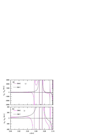
Figure 6: The polarizability difference between the $2\,^{2}\!S$ and $2\,^{2}\!P$ states of Li. Polarizability differences are shown for $M=0$ and $M=1$.

The dynamic polarizabilities for the Be⁺ $2\,^{2}\!P$ state are also tabulated in Table 4 and depicted in Figure 5 for the photon frequencies below 0.40 a.u.. There are three resonances in this frequency range. The scalar and tensor dynamic polarizabilities are similar in shape but with the opposite sign. As far as we know, there has been no previous calculation of the $2\,^{2}\!P$ state dynamic polarizability.

Figure 7: The polarizability difference between the $2\,^{2}\!S$ and $2\,^{2}\!P$ states of Be⁺. Polarizability differences are shown for $M=0$ and $M=1$.

III.3 The static $2\,^{2}\!S$ $\to$ $2\,^{2}\!P$ Stark shift

The static Stark shift for the $2\,^{2}\!S$ $\to$ $2\,^{2}\!P$ energy interval in an electric field of strength $F$ is written as

$$\Delta E_{\rm 2s-2p,M} = -\frac{1}{2}F^{2}\left(\alpha_{\rm 2s}-\alpha_{\rm 2p,M}\right)$$ (14)

$$- \frac{1}{24}F^{4}\left(\gamma_{\rm 2s}-\gamma_{\rm 2p,M}\right)+\ldots\,,$$

where $\gamma$ is the hyper-polarizability. The Stark shift depends on the magnetic quantum number $M$ of the $2\,^{2}\!P$ state. The relative size of $\Delta\alpha$ and $\Delta\gamma$ determines the extent to which the Stark shift is influenced by the hyper-polarizability at high field strengths. The relative importance of $\Delta\alpha$ and $\Delta\gamma$ is given by the ratio

$$X=\frac{F^{2}(\gamma_{2s}-\gamma_{2p,M})}{12(\alpha_{2s}-\alpha_{2p,M})}=\frac{F^{2}\Delta\gamma}{12\Delta\alpha}\,.$$ (15)

Using the static polarizability and static hyper-polarizability for the Li atom results in $\Delta\alpha=37.1$ and $\Delta\gamma=9.99\times 10^{6}$ giving $X=0.0001$ at $F=6.67\times 10^{-5}$ a.u. (344 kV/cm) and $X=0.001$ at $F=2.11\times 10^{-4}$ a.u. (1087 kV/cm). These estimates of the critical field strength where the quadratic Stark shift is valid depend slightly on the magnetic quantum number and exact values can be determined by using $M$-dependent polarizabilities. Stark shifts of higher order than the hyper-polarizability can be comfortably ignored at the 0.01$\%$ level provided the field strength is less than 1100 kV/cm. The static Stark shift for Be⁺ is not interesting since it is difficult to measure as a Be⁺ ion immersed in a finite electric field is accelerated away from the finite field region.

Table 5: The photon energies for which there is no Stark shift for the $2\,^{2}\!S$ $\to$ $2\,^{2}\!P$ transition. Underlined digits indicate uncertain digits arising from lack of basis set convergence. Digits in brackets indicate possible uncertainties associated with relativistic corrections in the recommended (Rec.) values.

System	$M=0$	$M=1$
∞Li	$0.046317680\underline{6}$	$0.084763957\underline{1}$
	$0.081021795\underline{5}$
	$0.093664330\underline{5}$
7Li	$0.046335687\underline{8}$	$0.084766087\underline{0}$
	$0.081024478\underline{9}$
	$0.093661899\underline{1}$
Rec. 7Li	$0.046297(4)$	$0.084756(2)$
	$0.081014(2)$
	$0.0936613(2)$
∞Be+	$0.262920267\underline{8}$	$0.378457000\underline{4}$
	$0.370371502\underline{7}$
	$0.390752146\underline{3}$
9Be+	$0.262917360\underline{3}$	$0.378451843\underline{7}$
	$0.370279952\underline{2}$
	$0.390455356\underline{8}$
Rec. 9Be+	$0.2628956(7)$	$0.378443(2)$
	$0.370274(1)$
	$0.3904546(2)$

III.4 The dynamic $2\,^{2}\!S$ $\to$ $2\,^{2}\!P$ Stark shift

The Li Stark shifts, $\alpha(2s)-\alpha(2p_{M})$, are plotted as a function of frequency in Figure 6. It is seen that there are magic wavelengths for $M=0$ just below the $2\,^{2}\!P$ $\to$ $3\,^{2}\!S$ threshold and between the $2\,^{2}\!S$ $\to$ $2\,^{2}\!P$ and $2\,^{2}\!P$ $\to$ $3\,^{2}\!D$ thresholds. The actual energies for which the polarizability difference is zero are given in Table 5. The Stark shifts get very large for frequencies between 0.058 and 0.070 a.u..

The Be⁺ Stark shifts, $\alpha(2s)-\alpha(2p_{M})$, are plotted as a function of frequency in Figure 7. The Stark shifts are much smaller in magnitude than the Li atom shifts. One difference from Li is that the Be⁺ shift has no zero for energies below the $2\,^{2}\!S$ $\to$ $2\,^{2}\!P$ threshold. The first zero in the Stark shift (excepting those related to a singularity) is at 0.263 a.u..

Table 6: The parameters for the calculation of the $2\,^{2}\!S$ state frequency-dependent polarizabilities of Li and Be⁺. The numbers in the square brackets denote powers of 10. The recommended (Rec.) results of the fourth and the seventh columns incorporate relativistic corrections.

Parameter	∞Li	7Li	Rec. 7Li	∞Be+	9Be+	Rec. 9Be+
$f_{2s\rightarrow 2p}$	0.746956$\underline{855381}$	0.746961$\underline{871867}$	0.747011$\underline{776131}$	0.4980674$\underline{22721}$	0.4980833$\underline{82699}$	0.4982270$\underline{10322}$
$\Delta E_{2s2p}$	0.06790379$\underline{1567}$	0.06789417$\underline{2078}$	0.06790605	0.14542988$\underline{4364}$	0.14540357$\underline{2344}$	0.14547806
$f_{2s\rightarrow 3p}$	0.00473$\underline{1019443}$	0.00473$\underline{7600312}$	0.00472$\underline{8028090}$	0.0832$\underline{43986131}$	0.0832$\underline{889414647}$	0.0832$\underline{09271939}$
$\Delta E_{2s3p}$	0.14090$\underline{9212964}$	0.14089$\underline{6165068}$	0.14090640	0.4396$\underline{29051730}$	0.4395$\underline{96005937}$	0.43966521
$f_{2s\rightarrow 4p}$	0.00496$\underline{0028680}$	0.00496$\underline{4714658}$		0.04$\underline{0874056901}$	0.04$\underline{0896543934}$
$\Delta E_{2s4p}$	0.166$\underline{756175058}$	0.166$\underline{742266938}$		0.54$\underline{6967693380}$	0.54$\underline{6934227760}$
$S(-2)$	1.697$\underline{71}$	1.698$\underline{63}$		0.37$\underline{9627}$	0.37$\underline{9781}$
$S(-4)$	21.$\underline{8714}$	21.$\underline{8888}$		0.5$\underline{13938}$	0.5$\underline{14207}$
$S(-6)$	4$\underline{28.809}$	4$\underline{29.237}$		0.9$\underline{79476}$	0.9$\underline{80088}$
$S(-8)$	9.$\underline{69364}[3]$	9.$\underline{70502}[3]$		2.$\underline{05322}$	2.$\underline{05469}$
$S(-10)$	2.$\underline{37008}[5]$	2.$\underline{37325}[5]$		4.$\underline{52145}$	4.$\underline{52508}$
$S(-12)$	6.$\underline{08098}[6]$	6.$\underline{09006}[6]$		1$\underline{0.2473}$	1$\underline{0.2564}$
$S(-14)$	1.$\underline{61032}[8]$	1.$\underline{61296}[8]$		2$\underline{3.6368}$	2$\underline{3.6596}$
$S(-16)$	4.$\underline{35760}[9]$	4.$\underline{36537}[9]$		5$\underline{5.1280}$	5$\underline{5.1852}$
$\eta_{1}$	2$\underline{7.0605}$	2$\underline{7.0643}$		2.$\underline{33229}$	2.$\underline{33246}$

III.5 Analytic representation

The utility of the present calculations can be increased by constructing a closed form expression for the dynamic polarizability. This is done by retaining the first $3$ terms in Eq. (7) explicitly and then expanding the energy denominator in the remainder. The expressions explicitly include oscillator strengths up to the $n=4$ principal quantum numbers. The closed form expression is

$$\alpha_{1}(\omega) = \left(\sum_{n=2}^{4}\frac{f_{2s\rightarrow np}}{\Delta E_{2snp}^{2}-\omega^{2}}\right)+S(-2)+\omega^{2}S(-4)$$ (16)

$$+ \omega^{4}S(-6)+\ldots+\omega^{14}S(-16)+C(\omega)$$

where

$$S(-m)=\sum_{n=5}\frac{f_{2s\rightarrow np}}{(\Delta E_{2snp})^{m}}\,,$$ (17)

$$C(\omega)=\frac{\eta_{1}\omega^{16}S(-16)}{1-\eta_{1}\omega^{2}}\,.$$ (18)

Here $f_{2s\rightarrow np}$ are the dipole oscillator strengths for the $2\,^{2}\!S\rightarrow n\,^{2}\!P$ transitions with transition energies $\Delta E_{2snp}$. The $S(-n)$ are the Cauchy moments of the remainder of the oscillator strength distribution and are independent of $\omega$. The $C(\omega)$ is an approximate term to represent the summation from the term $S(-18)$ to $S(\infty)$. The ratio, $\eta_{1}=S(-n-2)/S(-n)$, is assumed to be constant and its value is set at $S(-16)/S(-14)$. Numerical values of the various constants in Eq. (16) can be found in Table 6. Inclusion of the remainder term has greatly increased the precision of the analytic fit to the exact dynamic polarizability.

The analytic representation for the Li $2\,^{2}\!S$ state is accurate to 0.01 a.u. for $\omega\leqslant 0.1612$ a.u. and to an accuracy of 0.1 a.u. for $\omega\leqslant 0.1728$ a.u.. The dynamic polarizability for the Be⁺ $2\,^{2}\!S$ state maintains its accuracy over a larger $\omega$ range. It is accurate to 0.001 a.u. for $\omega\leqslant 0.543$ a.u., to 0.01 a.u. for $\omega\leqslant 0.58605$ a.u. and 0.1 a.u. for $\omega\leqslant 0.6$ a.u..

The presence of zeroes in the dynamic polarizability near the singularities means that the relative error in the analytic representation can get very large in a frequency range very close to the zeroes. Neglecting these localized regions with anomalously high relative uncertainties, the relative difference between the analytic representation and actual dynamic polarizability for the Li $2\,^{2}\!S$ state was less than 0.001% for $\omega\leqslant 0.1399$ a.u., 0.01% for $\omega\leqslant 0.1551$ a.u., and 0.1% for $\omega\leqslant 0.1651$ a.u.. The relative difference for the Be⁺ $2\,^{2}\!S$ state obtained by the variational Hylleraas method was less than 0.001% for $\omega\leqslant 0.4737$ a.u., 0.01% for $\omega\leqslant 0.5067$ a.u. and 0.1% for $\omega\leqslant 0.52575$ a.u.. The inclusion of the remainder term, $C(\omega)$ improved the accuracy of the analytic representation by one or two order of magnitude within the frequency range listed above.

The dynamic dipole polarizabilities of the $2\,^{2}\!P$ states of Li and Be⁺ have both scalar, $\alpha_{1}(\omega)$, and tensor, $\alpha_{1}^{T}(\omega)$, parts. The scalar part can be written

$$\alpha_{1}(\omega) = \sum_{n=2}^{4}\frac{f_{2p\rightarrow ns}}{\Delta E_{2pns}^{2}-\omega^{2}}+\sum_{n=3}^{4}\frac{f_{2p\rightarrow nd}}{\Delta E_{2pnd}^{2}-\omega^{2}}$$ (19)

$$+ S(-2)+\omega^{2}S(-4)+\omega^{4}S(-6)+\ldots$$

$$+ \omega^{14}S(-16)+C(\omega)\,,$$

where

$$S(-m) = \sum_{n=5}\frac{f_{2p\rightarrow ns}}{(\Delta E_{2pns})^{m}}+\sum_{n^{\prime}}\frac{f_{2p\rightarrow n^{\prime}P}}{(\Delta E_{2pn^{\prime}P})^{m}}$$ (20)

$$+ \sum_{n=5}\frac{f_{2p\rightarrow nd}}{(\Delta E_{2pnd})^{m}}\,.$$

The $2p\rightarrow n^{\prime}P$ excitation involves a core excitation and the intermediate state is an unnatural parity ${}^{2}\!P^{e}$ state. The tensor part is

$$\alpha^{T}_{1}(\omega) = -\sum_{n=2}^{4}\frac{f_{2p\rightarrow ns}}{\Delta E_{2pns}^{2}-\omega^{2}}-\frac{1}{10}\sum_{n=3}^{4}\frac{f_{2p\rightarrow nd}}{\Delta E_{2pnd}^{2}-\omega^{2}}$$ (21)

$$+ S^{T}(-2)+\omega^{2}S^{T}(-4)+\omega^{4}S^{T}(-6)+\ldots$$

$$+ \omega^{14}S^{T}(-16)+C^{T}(\omega)\,,$$

where

$$S^{T}(-m) = -\sum_{n=5}\frac{f_{2p\rightarrow ns}}{(\Delta E_{2pns})^{m}}+\frac{1}{2}\sum_{n^{\prime}}\frac{f_{2p\rightarrow n^{\prime}P}}{(\Delta E_{2pn^{\prime}P})^{m}}$$ (22)

$$- \frac{1}{10}\sum_{n=5}\frac{f_{2p\rightarrow nd}}{(\Delta E_{2pnd})^{m}}\,,$$

$$C^{T}(\omega)=\frac{\eta^{T}_{1}\omega^{16}S^{T}(-16)}{1-\eta^{T}_{1}\omega^{2}}\,,$$ (23)

where $f_{2p\rightarrow mL_{1}}$ means the oscillator strength from $2p$ state to $mL_{1}$ state transition. $S^{T}(-2)$, $S^{T}(-4)$, $S^{T}(-6)$ $\cdots$ are the coefficients corresponding to $\omega^{0}$, $\omega^{2}$, $\omega^{4}$ $\cdots$ terms of the tensor part. The remainder term, $C^{T}(\omega)$ is an approximate expression to take into account the $S^{T}(-18)$ $\to$ $S^{T}(\infty)$ summations. The factor $\eta^{T}_{1}$ is set to be $\eta^{T}_{1}=S(-16)/S(-14)$. All parameters in the analytic representation are given in Table 7.

The first two terms of Eqs. (19) and (21) include five resonances, which make the major contribution to the polarizability with the second term involving excitations to $D$ states being the most important. This is clearly seen in the Li $\alpha_{1}(\omega)$ of 185.542(5) a.u. at $\omega=0.04$ a.u.. The contribution of the first summation of Eq. (19) was $-8.8717$ a.u., while the second summation contributed 175.8241 a.u.. The value given by Eq. (19) was 185.5378 a.u., which agrees with the exact value at the level of 0.0004$\%$.

The analytic representation for the scalar polarizability $\alpha_{1}(\omega)$ of the Li $2\,^{2}\!P$ state is accurate to 0.01 a.u. for $\omega\leqslant 0.0855$ a.u. and to 0.1 a.u. for $\omega\leqslant 0.0937$ a.u.. The analytic representation for the tensor polarizability, $\alpha_{1}^{T}(\omega)$, is accurate to 0.01 a.u. for $\omega\leqslant 0.0926$ a.u. and to 0.10 a.u. for $\omega\leqslant 0.1$ a.u..

Table 7: The parameters defining the frequency-dependent polarizabilities of the $2\,^{2}\!P$ state of Li and Be⁺. The numbers in the square brackets denote powers of 10. The recommended (Rec.) results of the fourth and the seventh columns incorporate relativistic effects.

Parameter	∞Li	7Li	Rec. 7Li	∞Be+	9Be+	Rec. 9Be+
$f_{2p\rightarrow 2s}$	$-0.2489856\underline{18454}$	$-0.2489872\underline{90622}$	$-0.2490039\underline{2538}$	$-0.1660224\underline{74240}$	$-0.1660277\underline{94233}$	$-0.1660756\underline{70107}$
$\Delta E_{2p2s}$	$-0.06790379\underline{1567}$	$-0.06789417\underline{2078}$	$-0.067906050$	$-0.14542988\underline{4364}$	$-0.14540357\underline{2344}$	$-0.145478060000$
$f_{2p\rightarrow 3s}$	0.1105$\underline{78835460}$	0.1105$\underline{75403831}$	0.1105$\underline{89306872}$	0.0643$\underline{85095804}$	0.0643$\underline{85347515}$	0.0644$\underline{07168594}$
$\Delta E_{2p3s}$	0.05605$\underline{9306121}$	0.05605$\underline{8468507}$	0.056054150	0.25656$\underline{1561765}$	0.25656$\underline{1980308}$	0.256536125000
$f_{2p\rightarrow 4s}$	0.014$\underline{979087136}$	0.014$\underline{981586569}$		0.012$\underline{876689561}$	0.012$\underline{879003186}$
$\Delta E_{2p4s}$	0.0927$\underline{14410055}$	0.0927$\underline{11788029}$		0.387$\underline{472175091}$	0.387$\underline{469829948}$
$f_{2p\rightarrow 3d}$	0.638568$\underline{044661}$	0.638583$\underline{007678}$	0.638583$\underline{083728}$	0.63198$\underline{1700709}$	0.63205$\underline{9480294}$	0.63204$\underline{7210702}$
$\Delta E_{2p3d}$	0.07463298$\underline{9884}$	0.07463045$\underline{3329}$	0.074630150	0.3012792$\underline{33806}$	0.3012763$\underline{62793}$	0.301291440000
$f_{2p\rightarrow 4d}$	0.1227$\underline{46501135}$	0.1227$\underline{56411337}$		0.12271$\underline{1398708}$	0.12273$\underline{4598764}$
$\Delta E_{2p4d}$	0.098967$\underline{235189}$	0.098962$\underline{799378}$		0.39864$\underline{0164736}$	0.39863$\underline{1384564}$
$S(-2)$	16.8$\underline{408}$	16.8$\underline{447}$		1.075$\underline{95}$	1.076$\underline{28}$
$S(-4)$	97$\underline{4.832}$	97$\underline{5.135}$		3.69$\underline{533}$	3.69$\underline{658}$
$S(-6)$	6.4$\underline{0829}[4]$	6.4$\underline{1083}[4]$		14.9$\underline{422}$	14.9$\underline{479}$
$S(-8)$	4.4$\underline{8404}[6]$	4.4$\underline{8620}[6]$		64.3$\underline{838}$	64.4$\underline{113}$
$S(-10)$	3.2$\underline{6108}[8]$	3.2$\underline{6295}[8]$		288.$\underline{547}$	288.$\underline{684}$
$S(-12)$	2.4$\underline{3429}[10]$	2.4$\underline{3592}[10]$		132$\underline{8.18}$	132$\underline{8.87}$
$S(-14)$	1.8$\underline{5141}[12]$	1.8$\underline{5282}[12]$		62$\underline{32.21}$	62$\underline{35.79}$
$S(-16)$	1.4$\underline{2796}[14]$	1.4$\underline{2918}[14]$		296$\underline{67.5}$	296$\underline{85.9}$
$\eta_{1}$	77.$\underline{1282}$	77.$\underline{1354}$		4.$\underline{76034}$	4.$\underline{76058}$
$S^{T}(-2)$	$-2.7\underline{3075}$	$-2.7\underline{3118}$		$-0.15\underline{6423}$	$-0.15\underline{6454}$
$S^{T}(-4)$	$-15\underline{4.670}$	$-15\underline{4.702}$		$-0.54\underline{4987}$	$-0.54\underline{5110}$
$S^{T}(-6)$	$-9.8\underline{8199}[3]$	$-9.8\underline{8458}[3]$		$-2.10\underline{990}$	$-2.11\underline{044}$
$S^{T}(-8)$	$-6.\underline{71603}[5]$	$-6.\underline{71818}[5]$		$-8.\underline{71572}$	$-8.\underline{71824}$
$S^{T}(-10)$	$-4.\underline{73561}[7]$	$-4.\underline{73742}[7]$		$-37.\underline{5083}$	$-37.\underline{5206}$
$S^{T}(-12)$	$-3.\underline{42263}[9]$	$-3.\underline{42417}[9]$		$-16\underline{6.164}$	$-16\underline{6.226}$
$S^{T}(-14)$	$-2.\underline{51902}[11]$	$-2.\underline{52034}[11]$		$-7\underline{52.681}$	$-7\underline{53.003}$
$S^{T}(-16)$	$-1.\underline{88083}[13]$	$-1.\underline{88197}[13]$		$-34\underline{71.37}$	$-34\underline{73.06}$
$\eta^{T}_{1}$	74.$\underline{6651}$	74.$\underline{6713}$		4.$\underline{61201}$	4.$\underline{61228}$

The relative error in the analytic representation of $\alpha_{1}(\omega)$ for the $2\,^{2}\!P$ state of the Li atom is less than 0.001% for $\omega\leqslant 0.082$ a.u., 0.01% for $\omega\leqslant 0.0871$ a.u., and 0.1% for $\omega\leqslant 0.0906$ a.u.. The relative error of the analytic representation for $\alpha_{1}^{T}(\omega)$ is less than 0.001% for $\omega\leqslant 0.0815$ a.u., 0.01% for $\omega\leqslant 0.0932$ a.u., and 0.1% for $\omega\leqslant 0.0995$ a.u..

The dynamic polarizability of the Be⁺ $2\,^{2}\!P$ state maintains its accuracy over a larger range of $\omega$. It is accurate to 0.001 a.u. for $\omega\leqslant 0.3513$ a.u., to 0.01 a.u. for $\omega\leqslant 0.3837$ a.u. and 0.1 a.u. for $\omega\leqslant 0.4111$ a.u.. The absolute error for $\alpha_{1}^{T}(\omega)$ is 0.001 a.u. for $\omega\leqslant 0.3788$ a.u., 0.01 a.u. for $\omega\leqslant 0.4077$ a.u., and 0.1 a.u. for $\omega\leqslant 0.4291$ a.u..

The relative error between the analytic representation and Hylleraas values of $\alpha_{1}(\omega)$ for the Be⁺ $2\,^{2}\!P$ is less than 0.001$\%$ for $\omega\leqslant 0.332$ a.u., 0.01% for $\omega\leqslant 0.3536$ a.u. and $0.1\%$ for $\omega\leqslant 0.3708$ a.u.. The relative error for $\alpha_{1}^{T}(\omega)$ of the Be⁺ $2\,^{2}\!P$ state is less than 0.001% for $\omega\leqslant 0.3265$ a.u., 0.01% for $\omega\leqslant 0.3434$ a.u. and 0.1% for $\omega\leqslant 0.3534$ a.u..

IV Finite mass corrections

The effect of the finite mass was to decrease the Li atom and Be⁺ ion binding energies listed in the Table 1. Therefore, it is not surprisingly that the $\omega=0$ polarizabilities of the Li and Be⁺ ground states are increased in Tables  2 and 3. The overall changes of the $\omega=0$ polarizabilities are $0.03\%$ and $0.04\%$ for Li and Be⁺ respectively. The finite mass polarizabilities are larger than the infinite mass values at $\omega=0$ a.u.. These differences can be taken as indicative of the overall change in the polarizabilities at finite frequencies below the first excitation threshold. The differences are naturally larger near thresholds.

The finite mass effect for the Li $2\,^{2}\!P$ state increased its polarizability by 0.001$\%$ (Table 4) while decreasing the polarizability for the Be⁺ $2\,^{2}\!P$ state (Table 4) by 0.08$\%$. This behavior for Be⁺ is due to the $2\,^{2}\!P$ $\to$ $2\,^{2}\!S$ downward transition. The increased negative contribution from this transition is enough to outweigh the increased positive contributions from transitions to more highly excited states.

As a general rule, the magnitude of the polarizabilities for both upward and downward transitions increase for the finite mass calculations. The residual Cauchy moments $S(-n)$ in Table 6 and Table 7 all increase for the finite mass calculations since these are computed exclusively from upward transitions.

V Other effects and Uncertainties

V.1 Estimate of Relativistic effects

The major omission from the present calculation is the inclusion of relativistic effects. The larger part of the energy difference between the present finite mass calculations and the experimental binding energies in Table 1 is due to the omission of relativistic effects. Relativistic effects will alter the polarizability calculation in two ways. First, the energy differences will be changed. Generally, the binding energies of all states can be expected to be slightly larger. Secondly, there will be some changes in the reduced matrix elements. The wave functions for the $n\,^{2}\!S$ and $n\,^{2}\!P$ states can be expected to be slightly more compact since they are more tightly bound.

Correcting for the relativistic energy is simply a matter of replacing the theoretical energies in the sum rules by the experimental values. The spin-orbit weighted averages were used for states with $L\geq 1$. The corrections to the transition matrix elements are made by recourse to calculations using a semi-empirical model potential that supplements the potential field of a frozen Hartree-Fock (HF) core with a tunable polarization potential zhang ; tang2 ; mitroy . Polarizabilities for Li and Be⁺ computed with this approach reproduce Hylleraas calculation at the 0.1$\%$ accuracy level zhang ; tang ; tang2 .

The method used to estimate the relativistic effect upon matrix elements relies on comparing two very similar calculations. One calculation has its polarization potentials tuned to reproduce the finite mass energies of Table 1. The other calculation is tuned to give the experimental energies. The matrix elements for the low lying transitions that dominate the dynamic polarizabilities are then compared. The differences between the “finite-mass” calculation and the “experimental” calculations are then determined. These changes in the matrix elements are then applied as corrections to the set of Hylleraas matrix elements. The only matrix elements that are changed are those involving transitions inside the $2\,^{2}\!L$ and $3\,^{2}\!L$ level space. Transitions to these states dominate the $2\,^{2}\!S$ and $2\,^{2}\!P$ polarizabilities. The actual change in the Li $2\,^{2}\!S$ $\to$ $2\,^{2}\!P$ matrix element was a reduction of 0.0054$\%$. The reduction in the Be⁺ $2\,^{2}\!S$ $\to$ $2\,^{2}\!P$ matrix element was 0.011$\%$.

Using the new set of corrected matrix elements gives a ground state polarizability of 164.114 a.u. (Table 1). This represents a reduction of the polarizability by 0.047 a.u.. A coupled cluster calculation of the lithium ground state estimated that relativistic effects reduced its polarizability by 0.06 a.u. lim . The static polarizability of the $2\,^{2}\!P$ state of ⁷Li, namely 126.947 a.u., was increased to 126.970 a.u. (Table 4). This gives a Stark shift of $-$37.144 a.u., which is in agreement with the experiment of Hunter et al hunter which gave $-$37.14(2) for the ⁷Li $2\,^{2}\!S-2\,^{2}\!P_{1/2}$ Stark shift. Another calculation was made to check the $2\,^{2}\!P_{1/2}$:$2\,^{2}\!P_{3/2}$ polarizability difference. The MBPT-SD calculation gave a difference of 0.015 a.u. johnson . Doing two calculations tuned to give a $2\,^{2}\!P$ spin-orbit splitting of $1.77\times 10^{-6}$ a.u.. (the energy splitting in the MBPT-SD calculation johnson ) gave a polarizability difference of 0.0145 a.u.. A further test was made by examination of the line strengths of the Si³⁺ $3\,^{2}\!S-3\,^{2}\!P$ spin-orbit doublet. A MBPT-SD calculation gave a line strength ratio of 1.000524 (once angular momentum factors were removed) mitroy09a . Turning the core potential in a semi-empirical model based on the Schrodinger equation mitroy09a gave a value of 1.000618. The available evidence supports the conjecture that it is possible to use the energy differences between the Hylleraas and experimental energies to get an initial estimate of relativistic corrections for other properties such as the polarizability. The uncertainty in the correction would seem to be about 20$\%$. To a certain extent the cancelations involved in adding the finite mass and relativistic corrections together leads to polarizabilities that are close to the infinite mass polarizabilities.

The static polarizability of the Be⁺ ground state was reduced from 24.506 to 24.489 a.u.. This represents a reduction of 0.4$\%$. However, the static scalar polarizability of the $2\,^{2}\!P$ state increased from 2.0231 to 2.0285 a.u., an increase of 0.24$\%$. The static tensor polarizability changed from 5.8589 to 5.8528 a.u.. The heavier mass and larger nuclear charge means relativistic effects are substantially larger than finite mass corrections.

Dynamic polarizabilities and their analytic representations from the set of matrix elements with the estimate of the relativistic effect are listed in Tables 2 - 7 as the recommended values. The changes to analytic representation only involved changes in the oscillator strength and energy differences for a few states.

Table 8: Experimental $C_{3}$ values from analysis of the Li₂ spectrum and $C_{3}$ values from the Hylleraas calculations.

Source	Value
Li2 spectrum mcalexander , $C_{6}$ fixed from yan1	11.0022(24)
Li2 spectrum leroy , $C_{6}$ fixed from yan1	11.00241(23)
Li2 spectrum leroy , $C_{6}$ fixed from zhang	11.00240(23)
Hylleraas ∞Li	11.000221
Hylleraas 7Li	11.001853
Hylleraas 7Li: Recommended	11.0007

V.2 The $2\,^{2}\!S$ $\to$ $2\,^{2}\!P$ matrix element and uncertainties

Recently Le Roy et al leroy analysed the ro-vibrational spectrum of the lithium dimer obtaining an estimate for the $C_{3}$ parameter describing the long range $C_{3}/R^{3}$ potential of the A-state that dissociates to the $2\,^{2}\!S$ and $2\,^{2}\!P$ states. The $C_{3}$ parameter can be related to the $2\,^{2}\!S-2\,^{2}\!P$ multiplet strength. The determination of Le Roy et al represented an order of magnitude improvement in precision over any previous determination of $C_{3}$.

The current value of $C_{3}=11.0007$ a.u. computed with relativistic corrections is about 0.0155$\%$ smaller than the experimental value of Le Roy et al. The finite mass calculation with the relativistic correction is closer to experiment than the infinite mass $C_{3}$, but there is a remaining discrepancy of 0.0017 a.u.. It is not likely that QED effects can explain the discrepancy as Pachucki et al found that these were 2.5 times smaller than relativistic effects in the polarizability of helium pachucki . It must be recalled that the Le Roy et al experiment is reporting an order of magnitude improvement in experimental precision. Going to such extreme levels of precision means there might be small corrections that need to be applied to the analysis of the data that have not received consideration. For example, the value of $C_{3}$ will be different for states asymptotic to the $2\,^{2}\!P_{1/2}$ and $2\,^{2}\!P_{3/2}$ levels. The analysis of Le Roy et al uses a common $C_{3}$ value for both members of the spin-orbit doublet. Irrespective of this, it should be noted that experiment and theory are incompatible at precisions better than 0.01$\%$.

The difference between the present and Le Roy $C_{3}$ is used to assign an error to the present polarizability calculation. Changes of 0.008$\%$ were made to the $2(3)\,^{2}\!S-2(3)\,^{2}\!P$ matrix elements, the polarizabilities were recomputed, and the differences assigned as the uncertainty in the recommended values. This difference is actually larger than the estimated relativistic change in the matrix element. Therefore, the recommended static polarizability of the Li ground state is 164.11(3) a.u.. Uncertainties in the $2(3)\,^{2}\!P-3\,^{2}\!D$ matrix elements are smaller (relativistic effects have a smaller impact on these matrix elements) and have not been included in the uncertainty analysis. The final value for the static scalar polarizability of the $2\,^{2}\!P$ state was 126.970(4) a.u., while the tensor polarizability was 1.612(4) a.u..

The same uncertainty analysis was applied to the Be⁺ ion polarizabilities. The recommended value for the ground state is 24.489(4) a.u.. The static $2\,^{2}\!P$ scalar polarizability was set as 2.0285(10) a.u. while the tensor polarizability was set to 5.8528(10) a.u..

Uncertainties in the recommended dynamic polarizabilities in Tables 2, 3, 4 and 5 were computed by making corrections to the matrix elements, recomputing and then observing the change. These uncertainties are best interpreted as indicative as opposed to rigorous estimates.

VI Summary

Definitive non-relativistic values for the dynamic dipole polarizabilities of Li and Be⁺ in their low-lying $2\,^{2}\!S$ and $2\,^{2}\!P$ states have been established using the variational method with Hylleraas basis sets. Calculation for both finite and infinite nuclear mass systems have been performed. Analytic representations for the dynamic polarizabilities of the Li atom and the Be⁺ ion have also been developed. These results can serve as a standard against which any other calculation can be judged.

Subsidiary calculations have been used to estimate the impact of relativistic effects that are not explicitly included in the Hylleraas calculation. It is recommended that the value of 164.11(3) a.u. be adopted as the static polarizability of ⁷Li. The uncertainty of 0.03 a.u. is based on the difference between the present $C_{3}$ and that of Le Roy et al leroy . This accuracy level is also supported by the ⁷Li $2\,^{2}\!S-2\,^{2}\!P_{1/2}$ Stark shift of $-$37.14 a.u. which is in perfect agreement with the value of $-$37.14(2) given by the high precision experiment of Hunter et al hunter . The recommended static polarizability for Be⁺ is 24.489(4) a.u..

The dynamic polarizabilities that have been obtained can be used as an atom based standard for electromagnetic field intensity. These polarizabilities can be regarded as an initial attempt to develop atom based standards for polarizability and Stark shift measurements. The primary virtue of the method with which the relativistic corrections were evaluated was simplicity of computation. For present purposes, the estimate of the relativistic corrections only has to be accurate to 10-20$\%$ for the recommended polarizabilities to be valid. The comparisons that have been done with fully relativistic calculations suggest that the estimates of the relativistic corrections are indeed accurate at this level. However, a more rigorous estimate using the Briet-Pauli Hamiltonian and perturbation theory would be desirable pachucki ; cencek ; lach .

- (1) T. Rosenband, D. B. Hume, P. O. Schmidt, C. W. Chou, A. Brusch, L. Lorini, W. H. Oskay, R. E. Drullinger, T. M. Fortier, J. E. Stalnaker, S. A. Diddams, W. C. Swann, N. R. Newbury, W. M. Itano, D. J. Wineland, and J. C. Bergquist, Science. 319, 1808 (2008).
- (2) H. S. Margolis, G. P. Barwood, G. Huang, H. A. Klein, S. N. Lea, K. Szymaniec, and P. Gill, Science. 306, 1355 (2004).
- (3) M. Chwalla, J. Benhelm, K. Kim, G. Kirchmair, T. Monz, M. Riebe, P. Schindler, A. S. Villar, W. Hänsel, C. F. Roos, R. Blatt, M. Abgrall, G. Santarelli, G. D. Rovera, and Ph. Laurent, Phys. Rev. Lett. 102, 023002 (2009).
- (4) Z. W. Barber, J. E. Stalnaker, N. D. Lemke, N. Poli, C. W. Oates, T. M. Fortier, S. A. Diddams, L. Hollberg, C. W. Hoyt, A. V. Taichenachev, and V. I. Yudin, Phys. Rev. Lett. 100, 103002 (2008).
- (5) H. Katori, M. Takamoto, V. G. Pal’chikov, and V. D. Ovsiannikov, Phys. Rev. Lett. 91, 173005 (2003).
- (6) C. A. Stan, M. W. Zwierlein, C. H. Schunck, S. M. F. Raupach, and W. Ketterle, Phys. Rev. Lett. 93, 143001 (2004).
- (7) S. Inouye, J. Goldwin, M. L. Olsen, C. Ticknor, J. L. Bohn, and D. S. Jin, Phys. Rev. Lett. 93, 183201 (2004).
- (8) R. J. Le Roy, N. S. Dattani, J. A. Coxon, A. J. Ross, P. Crozet, and C. Linton, J. Chem. Phys. 131, 204309 (2009).
- (9) A. Miffre, M. Jacquey, M. Büchner, G. Trénec, and J. Vigué, Phys. Rev. A 73, 011603(R) (2006).
- (10) C. R. Ekstrom, J. Schmiedmayer, M. S. Chapman, T. D. Hammond, and D. E. Pritchard, Phys. Rev. A 51, 3883 (1995).
- (11) A. D. Cronin, J. Schmiedmayer, and D. E. Pritchard, Rev. Mod. Phys. 81, 1051 (2009).
- (12) K. E. Miller, D. Krause Jr., and L. R. Hunter, Phys. Rev. A 49, 5128 (1994).
- (13) L. R. Hunter, D. Krause, D. J. Berkeland, and M. G. Boshier, Phys. Rev. A 44, 6140 (1991).
- (14) L. R. Hunter, D. Krause, K. E. Miller, D. J. Berleland, and M. G. Boshier, Optics Communications 94, 210 (1992).
- (15) R. Ashby, J. J. Clarke, and W. A. van Wijngaarden, Eur. Phys. J. D 23, 327 (2003).
- (16) G. D. Stevens, C.-H. Iu, T. Bergeman, H. J. Metcalf, I. Seipp, K. T. Taylor, and D. Delande, Phys. Rev. Lett. 75, 3402 (1995).
- (17) L. Y. Tang, Z. C. Yan, T. Y. Shi, and J. F. Babb, Phys. Rev. A 79, 062712 (2009).
- (18) S. Cohen, and S. I. Themelis, J. Chem. Phys. 124, 134106 (2006).
- (19) Z. C. Yan, J. F. Babb, A. Dalgarno, and G. W. F. Drake, Phys. Rev. A 54, 2824 (1996).
- (20) J. Y. Zhang, J. Mitroy, and M. W. J. Bromley, Phys. Rev. A 75, 042509 (2007).
- (21) Z.-C. Yan, J. Y. Zhang, Y. Li, Phys. Rev. A 67, 062504 (2003).
- (22) W. R. Johnson, U. I. Safronova, A. Derevianko, and M. S. Safronova, Phys. Rev. A 77, 022510 (2008).
- (23) L. Y. Tang, J.Y. Zhang, Z. C. Yan, T. Y. Shi, J. F. Babb, and J. Mitroy, Phys. Rev. A 80, 042511 (2009).
- (24) D. K. McKenzie and G. W. F. Drake, Phys. Rev. A 44, R6973 (1991).
- (25) Z. C. Yan and G. W. F. Drake, J. Phys. B. 30, 4723 (1997).
- (26) J. Pipin, and D. M. Bishop, Phys. Rev. A 45, 2736 (1992).
- (27) M. Mérawa, M. Rérat, and C. Pouchan, Phys. Rev. A 49, 2493 (1994).
- (28) M. Mérawa, and M. Rérat, J. Chem. Phys. 108, 7060 (1998).
- (29) V. E. Chernov, D. L. Dorofeev, I. Yu. Kretinin, and B. A. Zon, Phys. Rev. A 71, 022505 (2005).
- (30) J. Muszynska, D. Papierowska, J. Pipin, and W. Woznicki, Int. Quantum Chem. 22, 1153 (1982).
- (31) T. Kobayashi, K. Sasagane, and K. Yamaguchi, Int. Quantum Chem. 65, 665 (1997).
- (32) M. S. Safronova, B. Arora, and C. W. Clark, Phys. Rev. A 73, 022505 (2006).
- (33) Y. Ralchenko, A. E. Kramida, J. Reader, and NIST ASD Team (2008). NIST Atomic Spectra Database (version 3.1.5), [Online]. Available: http://physics.nist.gov/asd3 [2009, September 17]. National Institute of Standards and Technology, Gaithersburg, MD.
- (34) G. W. F. Drake. Handbook of Atomic, Molecular, and Optical Physics (American Institute of Physics, New York, 1996).
- (35) J. Y. Zhang and Z. C. Yan, J. Phys. B 37, 723 (2004).
- (36) J. Mitroy, and M. W. J. Bromley, Phys. Rev. A 68, 052714 (2003).
- (37) I. S. Lim, M. Pernpointner, M. Seth, J. K. Laerdahl, P. Schwerdtfeger, P. Neogrady, and M. Urban, Phys. Rev. A 60, 2822 (1999).
- (38) J. Mitroy and M. S. Safronova, Phys. Rev. A. 79, 012513 (2009).
- (39) W. I. McAlexander, E. R. I. Abraham, and R. G. Hulet, Phys. Rev. A 54, R5 (1996).
- (40) K. Pachucki, and J. Sapirstein, Phys. Rev. A. 63, 012504 (2000).
- (41) G. Lach, B. Jeziorski and K. Szalewicz, Phys. Rev. Lett. 92, 233001 (2004).
- (42) W. Cencek, K. Szalewicz and B. Jeziorski, Phys. Rev. Lett. 86, 5675 (2001).