$\mathcal{X}$–Armed Bandits

Abstract

We consider a generalization of stochastic bandits where the set of arms, $\mathcal{X}$, is allowed to be a generic measurable space and the mean-payoff function is “locally Lipschitz” with respect to a dissimilarity function that is known to the decision maker. Under this condition we construct an arm selection policy, called HOO (hierarchical optimistic optimization), with improved regret bounds compared to previous results for a large class of problems. In particular, our results imply that if $\mathcal{X}$ is the unit hypercube in a Euclidean space and the mean-payoff function has a finite number of global maxima around which the behavior of the function is locally continuous with a known smoothness degree, then the expected regret of HOO is bounded up to a logarithmic factor by $\sqrt{n}$, i.e., the rate of growth of the regret is independent of the dimension of the space. We also prove the minimax optimality of our algorithm when the dissimilarity is a metric. Our basic strategy has quadratic computational complexity as a function of the number of time steps and does not rely on the doubling trick. We also introduce a modified strategy, which relies on the doubling trick but runs in linearithmic time. Both results are improvements with respect to previous approaches.

1 Introduction

In the classical stochastic bandit problem a gambler tries to maximize his revenue by sequentially playing one of a finite number of slot machines that are associated with initially unknown (and potentially different) payoff distributions [26]. Assuming old-fashioned slot machines, the gambler pulls the arms of the machines one by one in a sequential manner, simultaneously learning about the machines’ payoff-distributions and gaining actual monetary reward. Thus, in order to maximize his gain, the gambler must choose the next arm by taking into consideration both the urgency of gaining reward (“exploitation”) and acquiring new information (“exploration”).

Maximizing the total cumulative payoff is equivalent to minimizing the (total) regret, i.e., minimizing the difference between the total cumulative payoff of the gambler and the one of another clairvoyant gambler who chooses the arm with the best mean-payoff in every round. The quality of the gambler’s strategy can be characterized as the rate of growth of his expected regret with time. In particular, if this rate of growth is sublinear, the gambler in the long run plays as well as the clairvoyant gambler. In this case the gambler’s strategy is called Hannan consistent.

Bandit problems have been studied in the Bayesian framework [19], as well as in the frequentist parametric [25; 2] and non-parametric settings [4], and even in non-stochastic scenarios [5; 10]. While in the Bayesian case the question is whether the optimal actions can be computed efficiently, in the frequentist case the question is how to achieve low rate of growth of the regret in the lack of prior information, i.e., it is a statistical question. In this paper we consider the stochastic, frequentist, non-parametric setting.

Although the first papers studied bandits with a finite number of arms, researchers have soon realized that bandits with infinitely many arms are also interesting, as well as practically significant. One particularly important case is when the arms are identified by a finite number of continuous-valued parameters, resulting in online optimization problems over continuous finite-dimensional spaces. Such problems are ubiquitous to operations research and control. Examples are “pricing a new product with uncertain demand in order to maximize revenue, controlling the transmission power of a wireless communication system in a noisy channel to maximize the number of bits transmitted per unit of power, and calibrating the temperature or levels of other inputs to a reaction so as to maximize the yield of a chemical process” [12]. Other examples are optimizing parameters of schedules, rotational systems, traffic networks or online parameter tuning of numerical methods. During the last decades numerous authors have investigated such “continuum-armed” bandit problems [3; 21; 6; 22; 12]. A special case of interest, which forms a bridge between the case of a finite number of arms and the continuum-armed setting, is formed by bandit linear optimization, see [1] and the references therein.

In many of the above-mentioned problems, however, the natural domain of some of the optimization parameters is a discrete set, while other parameters are still continuous-valued. For example, in the pricing problem different product lines could also be tested while tuning the price, or in the case of transmission power control different protocols could be tested while optimizing the power. In other problems, such as in online sequential search, the parameter-vector to be optimized is an infinite sequence over a finite alphabet [13; 7].

The motivation for this paper is to handle all these various cases in a unified framework. More precisely, we consider a general setting that allows us to study bandits with almost no restriction on the set of arms. In particular, we allow the set of arms to be an arbitrary measurable space. Since we allow non-denumerable sets, we shall assume that the gambler has some knowledge about the behavior of the mean-payoff function (in terms of its local regularity around its maxima, roughly speaking). This is because when the set of arms is uncountably infinite and absolutely no assumptions are made on the payoff function, it is impossible to construct a strategy that simultaneously achieves sublinear regret for all bandits problems (see, e.g., [9, Corollary 4]). When the set of arms is a metric space (possibly with the power of the continuum) previous works have assumed either the global smoothness of the payoff function [3; 21; 22; 12] or local smoothness in the vicinity of the maxima [6]. Here, smoothness means that the payoff function is either Lipschitz or Hölder continuous (locally or globally). These smoothness assumptions are indeed reasonable in many practical problems of interest.

In this paper, we assume that there exists a dissimilarity function that constrains the behavior of the mean-payoff function, where a dissimilarity function is a measure of the discrepancy between two arms that is neither symmetric, nor reflexive, nor satisfies the triangle inequality. (The same notion was introduced simultaneously and independently of us by [23, Section 4.4] under the name “quasi-distance.”) In particular, the dissimilarity function is assumed to locally set a bound on the decrease of the mean-payoff function at each of its global maxima. We also assume that the decision maker can construct a recursive covering of the space of arms in such a way that the diameters of the sets in the covering shrink at a known geometric rate when measured with this dissimilarity.

Relation to the literature.

Our work generalizes and improves previous works on continuum-armed bandits.

In particular, Kleinberg [21] and Auer et al. [6] focused on one-dimensional problems, while we allow general spaces. In this sense, the closest work to the present contribution is that of Kleinberg et al. [22], who considered generic metric spaces assuming that the mean-payoff function is Lipschitz with respect to the (known) metric of the space; its full version [23] relaxed this condition and only requires that the mean-payoff function is Lipschitz at some maximum with respect to some (known) dissimilarity. Kleinberg et al. [23] proposed a novel algorithm that achieves essentially the best possible regret bound in a minimax sense with respect to the environments studied, as well as a much better regret bound if the mean-payoff function has a small “zooming dimension”.

Our contribution furthers these works in two ways:

 (i)

our algorithms, motivated by the recent successful tree-based optimization algorithms [24; 18; 13], are easy to implement;

(ii)

we show that a version of our main algorithm is able to exploit the local properties of the mean-payoff function at its maxima only, which, as far as we know, was not investigated in the approach of Kleinberg et al. [22, 23].

The precise discussion of the improvements (and drawbacks) with respect to the papers by Kleinberg et al. [22, 23] requires the introduction of somewhat extensive notations and is therefore deferred to Section 5. However, in a nutshell, the following can be said.

First, by resorting to a hierarchical approach, we are able to avoid the use of the doubling trick, as well as the need for the (covering) oracle, both of which the so-called zooming algorithm of Kleinberg et al. [22] relies on. This comes at the cost of slightly more restrictive assumptions on the mean-payoff function, as well as a more involved analysis. Moreover, the oracle is replaced by an a priori choice of a covering tree. In standard metric spaces, such as the Euclidean spaces, such trees are trivial to construct, though, in full generality they may be difficult to obtain when their construction must start from (say) a distance function only. We also propose a variant of our algorithm that has smaller computational complexity of order $n\ln n$ compared to the quadratic complexity $n^{2}$ of our basic algorithm. However, the cheaper algorithm requires the doubling trick to achieve an anytime guarantee (just like the zooming algorithm).

Second, we are also able to weaken our assumptions and to consider only properties of the mean-payoff function in the neighborhoods of its maxima; this leads to regret bounds scaling as $\widetilde{O}\bigl{(}\sqrt{n}\bigr{)}$ when, e.g., the space is the unit hypercube and the mean-payoff function has a finite number of global maxima $x^{*}$ around which it is locally equivalent to a function $\Arrowvert x-x^{*}\Arrowvert^{\alpha}$ with some known degree $\alpha>0$. Thus, in this case, we get the desirable property that the rate of growth of the regret is independent of the dimensionality of the input space. (Comparable dimensionality-free rates are obtained under different assumptions in [23].)

Finally, in addition to the strong theoretical guarantees, we expect our algorithm to work well in practice since the algorithm is very close to the recent, empirically very successful tree-search methods from the games and planning literature [16; 17; 27; 11; 15].

Outline.

The outline of the paper is as follows:

1. In Section 2 we formalize the $\mathcal{X}$–armed bandit problem.

2. In Section 3 we describe the basic strategy proposed, called HOO (hierarchical optimistic optimization).

3. We present the main results in Section 4. We start by specifying and explaining our assumptions (Section 4.1) under which various regret bounds are proved. Then we prove a distribution-dependent bound for the basic version of HOO (Section 4.2). A problem with the basic algorithm is that its computational cost increases quadratically with the number of time steps. Assuming the knowledge of the horizon, we thus propose a computationally more efficient variant of the basic algorithm, called truncated HOO and prove that it enjoys a regret bound identical to the one of the basic version (Section 4.3) while its computational complexity is only log-linear in the number of time steps. The first set of assumptions constrains the mean-payoff function everywhere. A second set of assumptions is therefore presented that puts constraints on the mean-payoff function only in a small vicinity of its global maxima; we then propose another algorithm, called local-HOO, which is proven to enjoy a regret again essentially similar to the one of the basic version (Section 4.4). Finally, we prove the minimax optimality of HOO in metric spaces (Section 4.5).

4. In Section 5 we compare the results of this paper with previous works.

2 Problem setup

A stochastic bandit problem ${\cal B}$ is a pair ${\cal B}=(\mathcal{X},M)$, where $\mathcal{X}$ is a measurable space of arms and $M$ determines the distribution of rewards associated with each arm. We say that $M$ is a bandit environment on $\mathcal{X}$. Formally, $M$ is an mapping $\mathcal{X}\rightarrow{\cal M}_{1}(\mathbb{R})$, where ${\cal M}_{1}(\mathbb{R})$ is the space of probability distributions over the reals. The distribution assigned to arm $x\in\mathcal{X}$ is denoted by $M_{x}$. We require that for each arm $x\in\mathcal{X}$, the distribution $M_{x}$ admits a first-order moment; we then denote by $f(x)$ its expectation (“mean payoff”),

$$f(x)=\int y\,\,dM_{x}(y)\,.$$

The mean-payoff function $f$ thus defined is assumed to be measurable. For simplicity, we shall also assume that all $M_{x}$ have bounded supports, included in some fixed bounded interval, say, the unit interval $[0,1]$. Then, $f$ also takes bounded values, in $[0,1]$.

A decision maker (the gambler of the introduction) that interacts with a stochastic bandit problem ${\cal B}$ plays a game at discrete time steps according to the following rules. In the first round the decision maker can select an arm $X_{1}\in\mathcal{X}$ and receives a reward $Y_{1}$ drawn at random from $M_{X_{1}}$. In round $n>1$ the decision maker can select an arm $X_{n}\in\mathcal{X}$ based on the information available up to time $n$, i.e., $(X_{1},Y_{1},\ldots,X_{n-1},Y_{n-1})$, and receives a reward $Y_{n}$ drawn from $M_{X_{n}}$, independently of $(X_{1},Y_{1},\ldots,X_{n-1},Y_{n-1})$ given $X_{n}$. Note that a decision maker may randomize his choice, but can only use information available up to the point in time when the choice is made.

Formally, a strategy of the decision maker in this game (“bandit strategy”) can be described by an infinite sequence of measurable mappings, $\varphi=(\varphi_{1},\varphi_{2},\ldots)$, where $\varphi_{n}$ maps the space of past observations,

$$\mathcal{H}_{n}=\bigl{(}\mathcal{X}\times[0,1]\bigr{)}^{n-1},$$

to the space of probability measures over $\mathcal{X}$. By convention, $\varphi_{1}$ does not take any argument. A strategy is called deterministic if for every $n$, $\varphi_{n}$ is a Dirac distribution.

The goal of the decision maker is to maximize his expected cumulative reward. Equivalently, the goal can be expressed as minimizing the expected cumulative regret, which is defined as follows. Let

$$f^{*}=\sup_{x\in\mathcal{X}}f(x)$$

be the best expected payoff in a single round. At round $n$, the cumulative regret of a decision maker playing ${\cal B}$ is

$$\widehat{R}_{n}=n\,f^{*}-\sum_{t=1}^{n}Y_{t},$$

i.e., the difference between the maximum expected payoff in $n$ rounds and the actual total payoff. In the sequel, we shall restrict our attention to the expected cumulative regret, which is defined as the expectation $\mathbb{E}[\widehat{R}_{n}]$ of the cumulative regret $\widehat{R}_{n}$.

Finally, we define the cumulative pseudo-regret as

$$R_{n}=n\,f^{*}-\sum_{t=1}^{n}f(X_{t})\,,$$

that is, the actual rewards used in the definition of the regret are replaced by the mean-payoffs of the arms pulled. Since (by the tower rule)

$$\mathbb{E}\bigl{[}Y_{t}\bigr{]}=\mathbb{E}\bigl{[}\mathbb{E}\left[Y_{t}|X_{t}\right]\bigr{]}=\mathbb{E}\bigl{[}f(X_{t})\bigr{]}\,,$$

the expected values $\mathbb{E}[\widehat{R}_{n}]$ of the cumulative regret and $\mathbb{E}[R_{n}]$ of the cumulative pseudo-regret are the same. Thus, we focus below on the study of the behavior of $\mathbb{E}\bigl{[}R_{n}\bigr{]}$.

Remark 1

As it is argued in [9], in many real-world problems, the decision maker is not interested in his cumulative regret but rather in its simple regret. The latter can be defined as follows. After $n$ rounds of play in a stochastic bandit problem $\mathcal{B}$, the decision maker is asked to make a recommendation $Z_{n}\in\mathcal{X}$ based on the $n$ obtained rewards $Y_{1},\ldots,Y_{n}$. The simple regret of this recommendation equals

$$r_{n}=f^{*}-f(Z_{n})\,.$$

In this paper we focus on the cumulative regret $R_{n}$, but all the results can be readily extended to the simple regret by considering the recommendation $Z_{n}=X_{T_{n}}$, where $T_{n}$ is drawn uniformly at random in $\{1,\ldots,n\}$. Indeed, in this case,

$$\mathbb{E}\bigl{[}r_{n}\bigr{]}\leqslant\frac{\mathbb{E}\bigl{[}R_{n}\bigr{]}}{n}\,,$$

as is shown in [9, Section 3].

3 The Hierarchical Optimistic Optimization (HOO) strategy

The HOO strategy (cf. Algorithm 1) incrementally builds an estimate of the mean-payoff function $f$ over $\mathcal{X}$. The core idea (as in previous works) is to estimate $f$ precisely around its maxima, while estimating it loosely in other parts of the space $\mathcal{X}$. To implement this idea, HOO maintains a binary tree whose nodes are associated with measurable regions of the arm-space $\mathcal{X}$ such that the regions associated with nodes deeper in the tree (further away from the root) represent increasingly smaller subsets of $\mathcal{X}$. The tree is built in an incremental manner. At each node of the tree, HOO stores some statistics based on the information received in previous rounds. In particular, HOO keeps track of the number of times a node was traversed up to round $n$ and the corresponding empirical average of the rewards received so far. Based on these, HOO assigns an optimistic estimate (denoted by $B$) to the maximum mean-payoff associated with each node. These estimates are then used to select the next node to “play”. This is done by traversing the tree, beginning from the root, and always following the node with the highest $B$–value (cf. lines 4–14 of Algorithm 1). Once a node is selected, a point in the region associated with it is chosen (line 16) and is sent to the environment. Based on the point selected and the received reward, the tree is updated (lines 18–33).

The tree of coverings which HOO needs to receive as an input is an infinite binary tree whose nodes are associated with subsets of $\mathcal{X}$. The nodes in this tree are indexed by pairs of integers $(h,i)$; node $(h,i)$ is located at depth $h\geqslant 0$ from the root. The range of the second index, $i$, associated with nodes at depth $h$ is restricted by $1\leqslant i\leqslant 2^{h}$. Thus, the root node is denoted by $(0,1)$. By convention, $(h+1,2i-1)$ and $(h+1,2i)$ are used to refer to the two children of the node $(h,i)$. Let $\mathcal{P}_{h,i}\subset\mathcal{X}$ be the region associated with node $(h,i)$. By assumption, these regions are measurable and must satisfy the constraints

$$\mathcal{P}_{0,1} =\mathcal{X}\,,$$ (1a)

$$\mathcal{P}_{h,i} =\mathcal{P}_{h+1,2i-1}\cup\mathcal{P}_{h,2i}\,,\quad \mbox{for all}\ h\geqslant 0\ \mbox{and}\ 1\leqslant i\leqslant 2^{h}.$$ (1b)

As a corollary, the regions $\mathcal{P}_{h,i}$ at any level $h\geqslant 0$ cover the space $\mathcal{X}$,

$$\mathcal{X}=\bigcup_{i=1}^{2^{h}}\,\mathcal{P}_{h,i}\,,$$

explaining the term “tree of coverings”.

In the algorithm listing the recursive computation of the $B$–values (lines 28–33) makes a local copy of the tree; of course, this part of the algorithm could be implemented in various other ways. Other arbitrary choices in the algorithm as shown here are how tie breaking in the node selection part is done (lines 9–12), or how a point in the region associated with the selected node is chosen (line 16). We note in passing that implementing these differently would not change our theoretical results.

Parameters:  Two real numbers $\nu_{1}>0$ and $\rho\in(0,1)$, a sequence $(\mathcal{P}_{h,i})_{h\geqslant 0,1\leqslant i\leqslant 2^{h}}$ of subsets of $\mathcal{X}$ satisfying the conditions (1a) and (1b).

Auxiliary function Leaf($\mathcal{T}$):  outputs a leaf of $\mathcal{T}$.

Initialization:  $\mathcal{T}=\bigl{\{}(0,1)\bigr{\}}$ and $B_{1,2}=B_{2,2}=+\infty$.

1:for $n=1,2,\ldots$ do $\triangleright$ Strategy HOO in round $n\geqslant 1$

2:     $(h,i)\leftarrow(0,1)$ $\triangleright$ Start at the root

3:     $P\leftarrow\{(h,i)\}$ $\triangleright$ $P$ stores the path traversed in the tree

4:     while $(h,i)\in\mathcal{T}$ do $\triangleright$ Search the tree $\mathcal{T}$

5:         if $B_{h+1,2i-1}>B_{h+1,2i}$  then $\triangleright$ Select the “more promising” child

6:              $(h,i)\leftarrow(h+1,2i-1)$

7:         else if $B_{h+1,2i-1}<B_{h+1,2i}$  then

8:              $(h,i)\leftarrow(h+1,2i)$

9:         else$\triangleright$ Tie-breaking rule

10:              $Z\sim{\rm Ber}(0.5)$ $\triangleright$ e.g., choose a child at random

11:              $(h,i)\leftarrow(h+1,2i-Z)$

12:         end if

13:         $P\leftarrow P\cup\{(h,i)\}$

14:     end while

15:     $(H,I)\leftarrow(h,i)$ $\triangleright$ The selected node

16:      Choose arm $X$ in $\mathcal{P}_{H,I}$ and play it $\triangleright$ Arbitrary selection of an arm

17:     Receive corresponding reward $Y$

18:     $\mathcal{T}\leftarrow\mathcal{T}\cup\{(H,I)\}$ $\triangleright$ Extend the tree

19:     for all $(h,i)\in P$  do $\triangleright$ Update the statistics $T$ and $\widehat{\mu}$ stored in the path

20:         $T_{h,i}\leftarrow T_{h,i}+1$ $\triangleright$ Increment the counter of node $(h,i)$

21:         $\widehat{\mu}_{h,i}\leftarrow\bigl{(}1-1/T_{h,i}\bigr{)}\widehat{\mu}_{h,i}+Y/T_{h,i}$ $\triangleright$ Update the mean $\widehat{\mu}_{h,i}$ of node $(h,i)$

22:     end for

23:     for all $(h,i)\in\mathcal{T}$  do $\triangleright$ Update the statistics $U$ stored in the tree

24:         $U_{h,i}\leftarrow\widehat{\mu}_{h,i}+\sqrt{(2\ln n)/{T_{h,i}}}+\nu_{1}\rho^{h}$ $\triangleright$ Update the $U$–value of node $(h,i)$

25:     end for

26:     $B_{H+1,2I-1}\leftarrow+\infty$ $\triangleright$ $B$–values of the children of the new leaf

27:     $B_{H+1,2I}\leftarrow+\infty$

28:     $\mathcal{T}^{\prime}\leftarrow\mathcal{T}$ $\triangleright$ Local copy of the current tree $\mathcal{T}$

29:     while $\mathcal{T}^{\prime}\neq\bigl{\{}(0,1)\bigr{\}}$ do $\triangleright$ Backward computation of the $B$–values

30:         $(h,i)\leftarrow\mbox{{Leaf}}(\mathcal{T}^{\prime})$ $\triangleright$ Take any remaining leaf

31:         $B_{h,i}\leftarrow\min\Bigl{\{}U_{h,i},\,\max\bigl{\{}B_{h+1,2i-1},B_{h+1,2i}\bigr{\}}\Bigr{\}}$ $\triangleright$ Backward computation

32:         $\mathcal{T}^{\prime}\leftarrow\mathcal{T}^{\prime}\setminus\bigl{\{}(h,i)\bigr{\}}$ $\triangleright$ Drop updated leaf $(h,i)$

33:     end while

34:end for

Algorithm 1  The HOO strategy

To facilitate the formal study of the algorithm, we shall need some more notation. In particular, we shall introduce time-indexed versions ($\mathcal{T}_{n}$, $(H_{n},I_{n})$, $X_{n}$, $Y_{n}$, $\widehat{\mu}_{h,i}(n)$, etc.) of the quantities used by the algorithm. The convention used is that the indexation by $n$ is used to indicate the value taken at the end of the $n^{\rm th}$ round.

In particular, $\mathcal{T}_{n}$ is used to denote the finite subtree stored by the algorithm at the end of round $n$. Thus, the initial tree is $\mathcal{T}_{0}=\{(0,1)\}$ and it is expanded round after round as

$$\mathcal{T}_{n}=\mathcal{T}_{n-1}\cup\{(H_{n},I_{n})\}\,,$$

where $(H_{n},I_{n})$ is the node selected in line 15. We call $(H_{n},I_{n})$ the node played in round $n$. We use $X_{n}$ to denote the point selected by HOO in the region associated with the node played in round $n$, while $Y_{n}$ denotes the received reward.

Node selection works by comparing $B$–values and always choosing the node with the highest $B$–value. The $B$–value, $B_{h,i}(n)$, at node $(h,i)$ by the end of round $n$ is an estimated upper bound on the mean-payoff function at node $(h,i)$. To define it we first need to introduce the average of the rewards received in rounds when some descendant of node $(h,i)$ was chosen (by convention, each node is a descendant of itself):

$$\widehat{\mu}_{h,i}(n)=\frac{1}{T_{h,i}(n)}\,\sum_{t=1}^{n}\,Y_{t}\,\mathbb{I}_{\{(H_{t},I_{t})\in\mathcal{C}(h,i)\}}\,.$$

Here, $\mathcal{C}(h,i)$ denotes the set of all descendants of a node $(h,i)$ in the infinite tree,

$$\mathcal{C}(h,i)=\bigl{\{}(h,i)\bigr{\}}\cup\mathcal{C}(h+1,2i-1)\cup\mathcal{C}(h+1,2i)\,,$$

and $T_{h,i}(n)$ is the number of times a descendant of $(h,i)$ is played up to and including round $n$, that is,

$$T_{h,i}(n)=\sum_{t=1}^{n}\mathbb{I}_{\{(H_{t},I_{t})\in\mathcal{C}(h,i)\}}\,.$$

A key quantity determining $B_{h,i}(n)$ is $U_{h,i}(n)$, an initial estimate of the maximum of the mean-payoff function in the region $\mathcal{P}_{h,i}$ associated with node $(h,i)$:

$$U_{h,i}(n)=\begin{cases}\widehat{\mu}_{h,i}(n)+\displaystyle{\sqrt{\frac{2\ln n}{T_{h,i}(n)}}}+\nu_{1}\rho^{h},&\text{if }T_{h,i}(n)>0;\vspace{.15cm}\\ +\infty,&\text{otherwise}.\end{cases}$$ (2)

In the expression corresponding to the case $T_{h,i}(n)>0$, the first term added to the average of rewards accounts for the uncertainty arising from the randomness of the rewards that the average is based on, while the second term, $\nu_{1}\rho^{h}$, accounts for the maximum possible variation of the mean-payoff function over the region $\mathcal{P}_{h,i}$. The actual bound on the maxima used in HOO is defined recursively by

$$B_{h,i}(n)=\begin{cases}\min\Bigl{\{}U_{h,i}(n),\,\max\bigl{\{}B_{h+1,2i-1}(n),B_{h+1,2i}(n)\bigr{\}}\Bigr{\}},&\text{if }(h,i)\in\mathcal{T}_{n};\\ +\infty,&\text{otherwise}.\end{cases}$$

The role of $B_{h,i}(n)$ is to put a tight, optimistic, high-probability upper bound on the best mean-payoff that can be achieved in the region $\mathcal{P}_{h,i}$. By assumption, $\mathcal{P}_{h,i}=\mathcal{P}_{h+1,2i-1}\cup\mathcal{P}_{h+1,2i}$. Thus, assuming that $B_{h+1,2i-1}(n)$ (resp., $B_{h+1,2i}(n)$) is a valid upper bound for region $\mathcal{P}_{h+1,2i-1}$ (resp., $\mathcal{P}_{h+1,2i}$), we see that $\max\bigl{\{}B_{h+1,2i-1}(n),B_{h+1,2i}(n)\bigr{\}}$ must be a valid upper bound for region $\mathcal{P}_{h,i}$. Since $U_{h,i}(n)$ is another valid upper bound for region $\mathcal{P}_{h,i}$, we get a tighter (less overoptimistic) upper bound by taking the minimum of these bounds.

Obviously, for leafs $(h,i)$ of the tree $\mathcal{T}_{n}$, one has $B_{h,i}(n)=U_{h,i}(n)$, while close to the root one may expect that $B_{h,i}(n)<U_{h,i}(n)$; that is, the upper bounds close to the root are expected to be less biased than the ones associated with nodes farther away from the root.

Note that at the beginning of round $n$, the algorithm uses $B_{h,i}(n-1)$ to select the node $(H_{n},I_{n})$ to be played (since $B_{h,i}(n)$ will only be available at the end of round $n$). It does so by following a path from the root node to an inner node with only one child or a leaf and finally considering a child $(H_{n},I_{n})$ of the latter; at each node of the path, the child with highest $B$–value is chosen, till the node $(H_{n},I_{n})$ with infinite $B$–value is reached.

Illustrations.

Figure 1 illustrates the computation done by HOO in round $n$, as well as the correspondence between the nodes of the tree constructed by the algorithm and their associated regions. Figure 2 shows trees built by running HOO for a specific environment.

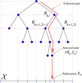
Figure 1: Illustration of the node selection procedure in round $n$. The tree represents $\mathcal{T}_{n}$. In the illustration, $B_{h+1,2i-1}(n-1)>B_{h+1,2i}(n-1)$, therefore, the selected path included the node $(h+1,2i-1)$ rather than the node $(h+1,2i)$.

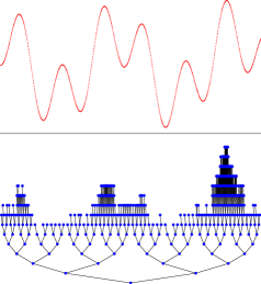
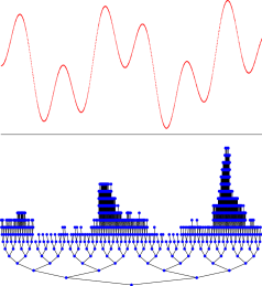
Figure 2: The trees (bottom figures) built by HOO after 1,000 (left) and 10,000 (right) rounds. The mean-payoff function (shown in the top part of the figure) is $x\in[0,1]\,\longmapsto\,1/2\bigl{(}\sin(13x)\sin(27x)+1\bigr{)}$; the corresponding payoffs are Bernoulli-distributed. The inputs of HOO are as follows: the tree of coverings is formed by all dyadic intervals, $\nu_{1}=1$ and $\rho=1/2$. The tie-breaking rule is to choose a child at random (as shown in the Algorithm 1), while the points in $\mathcal{X}$ to be played are chosen as the centers of the dyadic intervals. Note that the tree is extensively refined where the mean-payoff function is near-optimal, while it is much less developed in other regions.

Computational complexity.

At the end of round $n$, the size of the active tree $\mathcal{T}_{n}$ is at most $n$, making the storage requirements of HOO linear in $n$. In addition, the statistics and $B$–values of all nodes in the active tree need to be updated, which thus takes time $O(n)$. HOO runs in time $O(n)$ at each round $n$, making the algorithm’s total running time up to round $n$ quadratic in $n$. In Section 4.3 we modify HOO so that if the time horizon $n_{0}$ is known in advance, the total running time is $O(n_{0}\ln n_{0})$, while the modified algorithm will be shown to enjoy essentially the same regret bound as the original version.

4 Main results

We start by describing and commenting on the assumptions that we need to analyze the regret of HOO. This is followed by stating the first upper bound, followed by some improvements on the basic algorithm. The section is finished by the statement of our results on the minimax optimality of HOO.

4.1 Assumptions

The main assumption will concern the “smoothness” of the mean-payoff function. However, somewhat unconventionally, we shall use a notion of smoothness that is built around dissimilarity functions rather than distances, allowing us to deal with function classes of highly different smoothness degrees in a unified manner. Before stating our smoothness assumptions, we define the notion of a dissimilarity function and some associated concepts.

Definition 2 (Dissimilarity)

A dissimilarity $\ell$ over $\mathcal{X}$ is a non-negative mapping $\ell:\mathcal{X}^{2}\to\mathbb{R}$ satisfying $\ell(x,x)=0$ for all $x\in\mathcal{X}$.

Given a dissimilarity $\ell$, the diameter of a subset $A$ of $\mathcal{X}$ as measured by $\ell$ is defined by

$$\mathop{\mathrm{diam}}(A)=\sup_{x,y\in A}\ell(x,y)\,,$$

while the $\ell$–open ball of $\mathcal{X}$ with radius $\varepsilon>0$ and center $x\in\mathcal{X}$ is defined by

$$\mathcal{B}(x,\varepsilon)=\left\{\,y\in\mathcal{X}\,:\,\ell(x,y)<\varepsilon\,\right\}\,.$$

Note that the dissimilarity $\ell$ is only used in the theoretical analysis of HOO; the algorithm does not require $\ell$ as an explicit input. However, when choosing its parameters (the tree of coverings and the real numbers $\nu_{1}>0$ and $\rho<1$) for the (set of) two assumptions below to be satisfied, the user of the algorithm probably has in mind a given dissimilarity.

However, it is also natural to wonder what is the class of functions for which the algorithm (given a fixed tree) can achieve non-trivial regret bounds; a similar question for regression was investigated e.g., by Yang [28]. We shall indicate below how to construct a subset of such a class, right after stating our assumptions connecting the tree, the dissimilarity, and the environment (the mean-payoff function). Of these, Assumption A2. will be interpreted, discussed, and equivalently reformulated below into (4), a form that might be more intuitive. The form (3) stated below will turn out to be the most useful one in the proofs.

• Assumptions  Given the parameters of HOO, that is, the real numbers $\nu_{1}>0$ and $\rho\in(0,1)$ and the tree of coverings $(\mathcal{P}_{h,i})$, there exists a dissimilarity function $\ell$ such that the following two assumptions are satisfied.

  1. There exists $\nu_{2}>0$ such that for all integers $h\geqslant 0$,

     1. $\mathop{\mathrm{diam}}(\mathcal{P}_{h,i})\leqslant\nu_{1}\rho^{h}$ for all $i=1,\ldots,2^{h}$;

     2. for all $i=1,\ldots,2^{h}$, there exists $x^{\circ}_{h,i}\in\mathcal{P}_{h,i}$ such that

        $$\mathcal{B}_{h,i}\stackrel{{\scriptstyle\rm\scriptsize def}}{{=}}\mathcal{B}\bigl{(}x^{\circ}_{h,i},\,\nu_{2}\rho^{h}\bigr{)}\subset\mathcal{P}_{h,i}~{};$$

     3. $\mathcal{B}_{h,i}\cap\mathcal{B}_{h,j}=\emptyset$ for all $1\leqslant i<j\leqslant 2^{h}$.

  2. The mean-payoff function $f$ satisfies that for all $x,y\in\mathcal{X}$,

     $$f^{*}-f(y)\leqslant f^{*}-f(x)+\max\bigl{\{}f^{*}-f(x),\,\ell(x,y)\bigr{\}}\,.$$ (3)

We show next how a tree induces in a natural way first a dissimilarity and then a class of environments. For this, we need to assume that the tree of coverings $(\mathcal{P}_{h,i})$ –in addition to (1a) and (1b)– is such that the subsets $\mathcal{P}_{h,i}$ and $\mathcal{P}_{h,j}$ are disjoint whenever $1\leqslant i<j\leqslant 2^{h}$ and that none of them is empty. Then, each $x\in\mathcal{X}$ corresponds to a unique path in the tree, which can be represented as an infinite binary sequence $x_{0}x_{1}x_{2}\ldots$, where

$$x_{0} = \mathbb{I}_{\bigl{\{}x\in\mathcal{P}_{1,1+1}\bigr{\}}}\,,$$

$$x_{1} = \mathbb{I}_{\bigl{\{}x\in\mathcal{P}_{2,1+(2x_{0}+1)}\bigr{\}}}\,,$$

$$x_{2} = \mathbb{I}_{\bigl{\{}x\in\mathcal{P}_{3,1+(4x_{0}+2x_{1}+1)}\bigr{\}}}\,,$$

$$\ldots$$

For points $x,y\in\mathcal{X}$ with respective representations $x_{0}x_{1}\ldots$ and $y_{0}y_{1}\ldots$, we let

$$\ell(x,y)=(1-\rho)\nu_{1}\,\sum_{h=0}^{\infty}\mathbb{I}_{\{x_{h}\not=y_{h}\}}\rho^{h}\,.$$

It is not hard to see that this dissimilarity satisfies A1.. Thus, the associated class of environments ${\cal C}$ is formed by those with mean-payoff functions satisfying A2. with the so-defined dissimilarity. This is a “natural class” underlying the tree for which our tree-based algorithm can achieve non-trivial regret. (However, we do not know if this is the largest such class.)

In general, Assumption A1. ensures that the regions in the tree of coverings $(\mathcal{P}_{h,i})$ shrink exactly at a geometric rate. The following example shows how to satisfy A1. when the domain $\mathcal{X}$ is a $D$–dimensional hyper-rectangle and the dissimilarity is some positive power of the Euclidean (or supremum) norm.

Example 1

Assume that $\mathcal{X}$ is a $D$-dimension hyper-rectangle and consider the dissimilarity $\ell(x,y)=b\|x-y\|_{2}^{a}$, where $a>0$ and $b>0$ are real numbers and $\|\cdot\|_{2}$ is the Euclidean norm. Define the tree of coverings $(\mathcal{P}_{h,i})$ in the following inductive way: let $\mathcal{P}_{0,1}=\mathcal{X}$. Given a node $\mathcal{P}_{h,i}$, let $\mathcal{P}_{h+1,2i-1}$ and $\mathcal{P}_{h+1,2i}$ be obtained from the hyper-rectangle $\mathcal{P}_{h,i}$ by splitting it in the middle along its longest side (ties can be broken arbitrarily).

We now argue that Assumption A1. is satisfied. With no loss of generality we take $\mathcal{X}=[0,1]^{D}$. Then, for all integers $u\geqslant 0$ and $0\leqslant k\leqslant D-1$,

$$\mathop{\mathrm{diam}}(\mathcal{P}_{uD+k,1})=b\left(\frac{1}{2^{u}}\sqrt{D-\frac{3}{4}\,k}\right)^{a}\leqslant b\left(\frac{\sqrt{D}}{2^{u}}\right)^{\!a}\,.$$

It is now easy to see that Assumption A1. is satisfied for the indicated dissimilarity, e.g., with the choice of the parameters $\rho=2^{-a/D}$ and $\nu_{1}=b\,\bigl{(}2\sqrt{D}\bigr{)}^{a}$ for HOO, and the value $\nu_{2}=b/2^{a}$.

Example 2

In the same setting, with the same tree of coverings $(\mathcal{P}_{h,i})$ over $\mathcal{X}=[0,1]^{D}$, but now with the dissimilarity $\ell(x,y)=b\|x-y\|_{\infty}^{a}$, we get that for all integers $u\geqslant 0$ and $0\leqslant k\leqslant D-1$,

$$\mathop{\mathrm{diam}}(\mathcal{P}_{uD+k,1})=b\left(\frac{1}{2^{u}}\right)^{a}\,.$$

This time, Assumption A1. is satisfied, e.g., with the choice of the parameters $\rho=2^{-a/D}$ and $\nu_{1}=b\,2^{a}$ for HOO, and the value $\nu_{2}=b/2^{a}$.

The second assumption, A2., concerns the environment; when Assumption A2. is satisfied, we say that $f$ is weakly Lipschitz with respect to (w.r.t.) $\ell$. The choice of this terminology follows from the fact that if $f$ is $1$–Lipschitz w.r.t. $\ell$, i.e., for all $x,y\in\mathcal{X}$, one has $|f(x)-f(y)|\leqslant\ell(x,y)$, then it is also weakly Lipschitz w.r.t. $\ell$.

On the other hand, weak Lipschitzness is a milder requirement. It implies local (one-sided) $1$–Lipschitzness at any global maximum, since at any arm $x^{*}$ such that $f(x^{*})=f^{*}$, the criterion (3) rewrites to $f(x^{*})-f(y)\leqslant\ell(x^{*},y)$. In the vicinity of other arms $x$, the constraint is milder as the arm $x$ gets worse (as $f^{*}-f(x)$ increases) since the condition (3) rewrites to

$$\forall\,y\in\mathcal{X},\qquad f(x)-f(y)\leqslant\max\bigl{\{}f^{*}-f(x),\,\ell(x,y)\bigr{\}}\,.$$ (4)

Here is another interpretation of these two facts; it will be useful when considering local assumptions in Section 4.4 (a weaker set of assumptions). First, concerning the behavior around global maxima, Assumption A2. implies that for any set $\mathcal{A}\subset\mathcal{X}$ with $\sup_{x\in\mathcal{A}}f(x)=f^{*}$,

$$f^{*}-\inf_{x\in\mathcal{A}}f(x)\leqslant\mathop{\mathrm{diam}}(\mathcal{A}).$$ (5)

Second, it can be seen that Assumption A2. is equivalent to the following property: for all $x\in\mathcal{X}$ and $\varepsilon\geqslant 0$,

$$\mathcal{B}\bigl{(}x,\,f^{*}-f(x)+\varepsilon\bigr{)}\,\subset\,\mathcal{X}_{2\bigl{(}f^{*}-f(x)\bigr{)}+\varepsilon}$$ (6)

where

$$\mathcal{X}_{\varepsilon}=\bigl{\{}x\in\mathcal{X}:f(x)\geqslant f^{*}-\varepsilon\bigr{\}}$$

denotes the set of $\varepsilon$–optimal arms. This second property essentially states that there is no sudden and large drop in the mean-payoff function around the global maxima (note that this property can be satisfied even for discontinuous functions).

Figure 3 presents an illustration of the two properties discussed above.

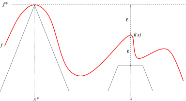
Figure 3: Illustration of the property of weak Lipschitzness (on the real line and for the distance $\ell(x,y)=|x-y|$). Around the optimum $x^{*}$ the values $f(y)$ should be above $f^{*}-\ell(x^{*},y)$. Around any $\varepsilon$–optimal point $x$ the values $f(y)$ should be larger than $f^{*}-2\varepsilon$ for $\ell(x,y)\leqslant\varepsilon$ and larger than $f(x)-\ell(x,y)$ elsewhere.

Before stating our main results, we provide a straightforward, though useful consequence of Assumptions A1. and A2., which should be seen as an intuitive justification for the third term in (2).

For all nodes $(h,i)$, let

$$f^{*}_{h,i}=\sup_{x\in\mathcal{P}_{h,i}}f(x)\qquad\mbox{and}\qquad\Delta_{h,i}=f^{*}-f^{*}_{h,i}\,.$$

$\Delta_{h,i}$ is called the suboptimality factor of node $(h,i)$. Depending whether it is positive or not, a node $(h,i)$ is called suboptimal ($\Delta_{h,i}>0$) or optimal ($\Delta_{h,i}=0$).

Lemma 3

Under Assumptions A1. and A2., if the suboptimality factor $\Delta_{h,i}$ of a region $\mathcal{P}_{h,i}$ is bounded by $c\nu_{1}\rho^{h}$ for some $c\geqslant 0$, then all arms in $\mathcal{P}_{h,i}$ are $\max\{2c,c+1\}\,\nu_{1}\rho^{h}$–optimal, that is,

$$\mathcal{P}_{h,i}\subset\mathcal{X}_{\max\{2c,c+1\}\,\nu_{1}\rho^{h}}\,.$$

Proof  For all $\delta>0$, we denote by $x^{*}_{h,i}(\delta)$ an element of $\mathcal{P}_{h,i}$ such that

$$f\bigl{(}x^{*}_{h,i}(\delta)\bigr{)}\geqslant f_{h,i}^{*}-\delta=f^{*}-\Delta_{h,i}-\delta\,.$$

By the weak Lipschitz property (Assumption A2.), it then follows that for all $y\in\mathcal{P}_{h,i}$,

$$f^{*}-f(y)\leqslant f^{*}-f\bigl{(}x^{*}_{h,i}(\delta)\bigr{)}+\max\Bigl{\{}f^{*}-f\bigl{(}x^{*}_{h,i}(\delta)\bigr{)},\,\ell\bigl{(}x^{*}_{h,i}(\delta),\,\,y\bigr{)}\Bigr{\}}\\ \leqslant\Delta_{h,i}+\delta+\max\bigl{\{}\Delta_{h,i}+\delta,\,\,\mathop{\mathrm{diam}}\mathcal{P}_{h,i}\bigr{\}}\,.$$ (7)

Letting $\delta\to 0$ and substituting the bounds on the suboptimality and on the diameter of $\mathcal{P}_{h,i}$ (Assumption A1) concludes the proof.  

4.2 Upper bound for the regret of HOO

Auer et al. [6, Assumption 2] observed that the regret of a continuum-armed bandit algorithm should depend on how fast the volumes of the sets of $\varepsilon$–optimal arms shrink as $\varepsilon\rightarrow 0$. Here, we capture this by defining a new notion, the near-optimality dimension of the mean-payoff function. The connection between these concepts, as well as with the zooming dimension defined by Kleinberg et al. [22], will be further discussed in Section 5. We start by recalling the definition of packing numbers.

Definition 4 (Packing number)

The $\varepsilon$–packing number $\mathcal{N}(\mathcal{X},\ell,\varepsilon)$ of $\mathcal{X}$ w.r.t. the dissimilarity $\ell$ is the size of the largest packing of $\mathcal{X}$ with disjoint $\ell$–open balls of radius $\varepsilon$. That is, $\mathcal{N}(\mathcal{X},\ell,\varepsilon)$ is the largest integer $k$ such that there exists $k$ disjoint $\ell$–open balls with radius $\varepsilon$ contained in $\mathcal{X}$.

We now define the $c$–near-optimality dimension, which characterizes the size of the sets $\mathcal{X}_{c\varepsilon}$ as a function of $\varepsilon$. It can be seen as some growth rate in $\varepsilon$ of the metric entropy (measured in terms of $\ell$ and with packing numbers rather than covering numbers) of the set of $c\varepsilon$–optimal arms.

Definition 5 (Near-optimality dimension)

For $c>0$ the $c$–near-optimality dimension of $f$ w.r.t. $\ell$ equals

$$\max\left\{0,\;\limsup_{\varepsilon\to 0}\frac{\ln\,\mathcal{N}\bigl{(}\mathcal{X}_{c\varepsilon},\ell,\,\varepsilon\bigl{)}}{\ln\bigl{(}\varepsilon^{-1}\bigr{)}}\right\}\,.$$

The following example shows that using a dissimilarity (rather than a metric, for instance) may sometimes allow for a significant reduction of the near-optimality dimension.

Example 3

Let $\mathcal{X}=[0,1]^{D}$ and let $f:[0,1]^{D}\rightarrow[0,1]$ be defined by $f(x)=1-\|x\|^{a}$ for some $a\geqslant 1$ and some norm $\|\cdot\|$ on $\mathbb{R}^{D}$. Consider the dissimilarity $\ell$ defined by $\ell(x,y)=\|x-y\|^{a}$. We shall see in Example 4 that $f$ is weakly Lipschitz w.r.t. $\ell$ (in a sense however slightly weaker than the one given by (5) and (6) but sufficiently strong to ensure a result similar to the one of the main result, Theorem 6 below). Here we claim that the $c$–near-optimality dimension (for any $c>0$) of $f$ w.r.t. $\ell$ is $0$. On the other hand, the $c$–near-optimality dimension (for any $c>0$) of $f$ w.r.t. the dissimilarity $\ell^{\prime}$ defined, for $0<b<a$, by $\ell^{\prime}(x,y)=\|x-y\|^{b}$ is $(1/b-1/a)D>0$. In particular, when $a>1$ and $b=1$, the $c$–near-optimality dimension is $(1-1/a)D$.

Proof  (sketch) Fix $c>0$. The set $\mathcal{X}_{c\varepsilon}$ is the $\|\cdot\|$–ball with center $0$ and radius $(c\varepsilon)^{1/a}$, that is, the $\ell$–ball with center $0$ and radius $c\varepsilon$. Its $\varepsilon$–packing number w.r.t. $\ell$ is bounded by a constant depending only on $D$, $c$ and $a$; hence, the value $0$ for the near-optimality dimension w.r.t. the dissimilarity $\ell$.

In case of $\ell^{\prime}$, we are interested in the packing number of the $\|\cdot\|$–ball with center $0$ and radius $(c\varepsilon)^{1/a}$ w.r.t. $\ell^{\prime}$–balls. The latter is of the order of

$$\left(\frac{(c\varepsilon)^{1/a}}{\varepsilon^{1/b}}\right)^{D}=c^{D/a}\bigl{(}\varepsilon^{-1}\bigr{)}^{(1/b-1/a)D}~{};$$

hence, the value $(1/b-1/a)D$ for the near-optimality dimension in the case of the dissimilarity $\ell^{\prime}$.

Note that in all these cases the $c$–near-optimality dimension of $f$ is independent of the value of $c$.  

We can now state our first main result. The proof is presented in Section A.1.

Theorem 6 (Regret bound for HOO)

Consider HOO tuned with parameters such that Assumptions A1. and A2. hold for some dissimilarity $\ell$. Let $d$ be the $4\nu_{1}/\nu_{2}$–near-optimality dimension of the mean-payoff function $f$ w.r.t.  $\ell$. Then, for all $d^{\prime}>d$, there exists a constant $\gamma$ such that for all $n\geqslant 1$,

$$\mathbb{E}\bigl{[}R_{n}\bigr{]}\leqslant\gamma\,n^{(d^{\prime}+1)/(d^{\prime}+2)}\,\bigl{(}\ln n\bigr{)}^{1/(d^{\prime}+2)}.$$

Note that if $d$ is infinite, then the bound is vacuous. The constant $\gamma$ in the theorem depends on $d^{\prime}$ and on all other parameters of HOO and of the assumptions, as well as on the bandit environment $M$. (The value of $\gamma$ is determined in the analysis; it is in particular proportional to $\nu_{2}^{-d^{\prime}}$.) The next section will exhibit a refined upper bound with a more explicit value of $\gamma$ in terms of all these parameters.

Remark 7

The tuning of the parameters of HOO is critical for the assumptions to be satisfied, thus to achieve a good regret; given some environment, one should select the parameters of HOO such that the near-optimality dimension of the mean-payoff function is minimized. Since the mean-payoff function is unknown to the user, this might be difficult to achieve. Thus, ideally, these parameters should be selected adaptively based on the observation of some preliminary sample. For now, the investigation of this possibility is left for future work.

4.3 Improving the running time when the time horizon is known

A deficiency of the basic HOO algorithm is that its computational complexity scales quadratically with the number of time steps. In this section we propose a simple modification to HOO that achieves essentially the same regret as HOO and whose computational complexity scales only log-linearly with the number of time steps. The needed amount of memory is still linear. We work out the case when the time horizon, $n_{0}$, is known in advance. The case of unknown horizon can be dealt with by resorting to the so-called doubling trick, see, e.g., [10, Section 2.3], which consists of periodically restarting the algorithm for regimes of lengths that double at each such fresh start, so that the $r^{\rm th}$ instance of the algorithm runs for $2^{r}$ rounds.

We consider two modifications to the algorithm described in Section 3. First, the quantities $U_{h,i}(n)$ of (2) are redefined by replacing the factor $\ln n$ by $\ln n_{0}$, that is, now

$$U_{h,i}(n)=\widehat{\mu}_{h,i}(n)+\sqrt{\frac{2\ln n_{0}}{T_{h,i}(n)}}+\nu_{1}\rho^{h}\,.$$

(This results in a policy which explores the arms with a slightly increased frequency.) The definition of the $B$–values in terms of the $U_{h,i}(n)$ is unchanged. A pleasant consequence of the above modification is that the $B$–value of a given node changes only when this node is part of a path selected by the algorithm. Thus at each round $n$, only the nodes along the chosen path need to be updated according to the obtained reward.

However, and this is the reason for the second modification, in the basic algorithm, a path at round $n$ may be of length linear in $n$ (because the tree could have a depth linear in $n$). This is why we also truncate the trees $\mathcal{T}_{n}$ at a depth $D_{n_{0}}$ of the order of $\ln n_{0}$. More precisely, the algorithm now selects the node $(H_{n},I_{n})$ to pull at round $n$ by following a path in the tree $\mathcal{T}_{n-1}$, starting from the root and choosing at each node the child with the highest $B$–value (with the new definition above using $\ln n_{0}$), and stopping either when it encounters a node which has not been expanded before or a node at depth equal to

$$D_{n_{0}}=\left\lceil\frac{(\ln n_{0})/2-\ln(1/\nu_{1})}{\ln(1/\rho)}\right\rceil\,.$$

(It is assumed that $n_{0}>1/\nu_{1}^{2}$ so that $D_{n_{0}}\geqslant 1$.) Note that since no child of a node $(D_{n_{0}},i)$ located at depth $D_{n_{0}}$ will ever be explored, its $B$–value at round $n\leqslant n_{0}$ simply equals $U_{D_{n_{0}},i}(n)$.

We call this modified version of HOO the truncated HOO algorithm. The computational complexity of updating all $B$–values at each round $n$ is of the order of $D_{n_{0}}$ and thus of the order of $\ln n_{0}$. The total computational complexity up to round $n_{0}$ is therefore of the order of $n_{0}\ln n_{0}$, as claimed in the introduction of this section.

As the next theorem indicates this new procedure enjoys almost the same cumulative regret bound as the basic HOO algorithm.

Theorem 8 (Upper bound on the regret of truncated HOO)

Fix a horizon $n_{0}$ such that $D_{n_{0}}\geqslant 1$. Then, the regret bound of Theorem 6 still holds true at round $n_{0}$ for truncated HOO up to an additional additive $4\sqrt{n_{0}}$ factor.

4.4 Local assumptions

In this section we further relax the weak Lipschitz assumption and require it only to hold locally around the maxima. Doing so, we will be able to deal with an even larger class of functions and in fact we will show that the algorithm studied in this section achieves a $O(\sqrt{n})$ bound on the regret regret when it is used for functions that are smooth around their maxima (e.g., equivalent to $\Arrowvert x-x^{*}\Arrowvert^{\alpha}$ for some known smoothness degree $\alpha>0$).

For the sake of simplicity and to derive exact constants we also state in a more explicit way the assumption on the near-optimality dimension. We then propose a simple and efficient adaptation of the HOO algorithm suited for this context.

4.4.1 Modified set of assumptions

• Assumptions  Given the parameters of (the adaption of) HOO, that is, the real numbers $\nu_{1}>0$ and $\rho\in(0,1)$ and the tree of coverings $(\mathcal{P}_{h,i})$, there exists a dissimilarity function $\ell$ such that Assumption A1. (for some $\nu_{2}>0$) as well as the following two assumptions hold.

  1. There exists $\varepsilon_{0}>0$ such that for all optimal subsets $\mathcal{A}\subset\mathcal{X}$ (i.e., $\sup_{x\in\mathcal{A}}f(x)=f^{*}$) with diameter $\mathop{\mathrm{diam}}(\mathcal{A})\leqslant\varepsilon_{0}$,

     $$f^{*}-\inf_{x\in\mathcal{A}}f(x)\leqslant\mathop{\mathrm{diam}}(\mathcal{A})\,.$$

     Further, there exists $L>0$ such that for all $x\in\mathcal{X}_{\varepsilon_{0}}$ and $\varepsilon\in[0,\varepsilon_{0}]$,

     $$\mathcal{B}\bigl{(}x,\,\,f^{*}-f(x)+\varepsilon\bigr{)}\,\subset\,\mathcal{X}_{L\bigl{(}2(f^{*}-f(x))+\varepsilon\bigr{)}}\,.$$

  2. There exist $C>0$ and $d>0$ such that for all $\varepsilon\leqslant\varepsilon_{0}$,

     $$\mathcal{N}\bigl{(}\mathcal{X}_{c\varepsilon},\,\ell,\,\varepsilon\bigr{)}\leqslant C\varepsilon^{-d}\,,$$

     where $c=4L\nu_{1}/\nu_{2}$.

When $f$ satisfies Assumption A2’., we say that $f$ is $\varepsilon_{0}$–locally $L$–weakly Lipschitz w.r.t.  $\ell$. Note that this assumption was obtained by weakening the characterizations (5) and (6) of weak Lipschitzness.

Assumption A3. is not a real assumption but merely a reformulation of the definition of near optimality (with the small added ingredient that the limit can be achieved, see the second step of the proof of Theorem 6 in Section A.1).

Example 4

We consider again the domain $\mathcal{X}$ and function $f$ studied in Example 3 and prove (as announced beforehand) that $f$ is $\varepsilon_{0}$–locally $2^{a-1}$–weakly Lipschitz w.r.t.  the dissimilarity $\ell$ defined by $\ell(x,y)=\|x-y\|^{a}$; which, in fact, holds for all $\varepsilon_{0}$.

Proof  Note that $x^{*}=(0,\ldots,0)$ is such that $f^{*}=1=f(x^{*})$. Therefore, for all $x\in\mathcal{X}$,

$$f^{*}-f(x)=\|x\|^{a}=\ell(x^{*},x)\,,$$

which yields the first part of Assumption A2’.. To prove that the second part is true for $L=2^{a-1}$ and with no constraint on the considered $\varepsilon$, we first note that since $a\geqslant 1$, it holds by convexity that $(u+v)^{a}\leqslant 2^{a-1}(u^{a}+v^{a})$ for all $u,v\geqslant 0$. Now, for all $\varepsilon\geqslant 0$ and $y\in\mathcal{B}\bigl{(}x,\,\|x\|^{a}+\varepsilon\bigr{)}$, i.e., $y$ such that $\ell(x,y)=\|x-y\|^{a}\leqslant\|x\|^{a}+\varepsilon$,

$$f^{*}-f(y)=\|y\|^{a}\leqslant\bigl{(}\|x\|+\|x-y\|\bigr{)}^{a}\leqslant 2^{a-1}\bigl{(}\|x\|^{a}+\|x-y\|^{a}\bigr{)}\leqslant 2^{a-1}\bigl{(}2\|x\|^{a}+\varepsilon\bigr{)}\,,$$ (8)

which concludes the proof of the second part of A2’..  

4.4.2 Modified HOO algorithm

We now describe the proposed modifications to the basic HOO algorithm.

We first consider, as a building block, the algorithm called $z$–HOO, which takes an integer $z$ as an additional parameter to those of HOO. Algorithm $z$–HOO works as follows: it never plays any node with depth smaller or equal to $z-1$ and starts directly the selection of a new node at depth $z$. To do so, it first picks the node at depth $z$ with the best $B$–value, chooses a path and then proceeds as the basic HOO algorithm. Note in particular that the initialization of this algorithm consists (in the first $2^{z}$ rounds) in playing once each of the $2^{z}$ nodes located at depth $z$ in the tree (since by definition a node that has not been played yet has a $B$–value equal to $+\infty$). We note in passing that when $z=0$, algorithm $z$–HOO coincides with the basic HOO algorithm.

Algorithm local-HOO employs the doubling trick in conjunction with consecutive instances of $z$–HOO. It works as follows. The integers $r\geqslant 1$ will index different regimes. The $r^{\rm th}$ regime starts at round $2^{r}-1$ and ends when the next regime starts; it thus lasts for $2^{r}$ rounds. At the beginning of regime $r$, a fresh copy of $z_{r}$–HOO, where $z_{r}=\lceil\log_{2}r\rceil$, is initialized and is then used throughout the regime.

Note that each fresh start needs to pull each of the $2^{z_{r}}$ nodes located at depth $z_{r}$ at least once (the number of these nodes is $\approx r$). However, since round $r$ lasts for $2^{r}$ time steps (which is exponentially larger than the number of nodes to explore), the time spent on the initialization of $z_{r}$–HOO in any regime $r$ is greatly outnumbered by the time spent in the rest of the regime.

In the rest of this section, we propose first an upper bound on the regret of $z$–HOO (with exact and explicit constants). This result will play a key role in proving a bound on the performance of local-HOO.

4.4.3 Adaptation of the regret bound

In the following we write $h_{0}$ for the smallest integer such that

$$2\nu_{1}\rho^{h_{0}}<\varepsilon_{0}$$

and consider the algorithm $z$–HOO, where $z\geqslant h_{0}$. In particular, when $z=0$ is chosen, the obtained bound is the same as the one of Theorem 6, except that the constants are given in analytic forms.

Theorem 9 (Regret bound for $z$–HOO)

Consider $z$–HOO tuned with parameters $\nu_{1}$ and $\rho$ such that Assumptions A1., A2’. and A3. hold for some dissimilarity $\ell$ and the values $\nu_{2},\,L,\,\varepsilon_{0},\,C,\,d$. If, in addition, $z\geqslant h_{0}$ and $n\geqslant 2$ is large enough so that

$$z\leqslant\frac{1}{d+2}\frac{\ln(4L\nu_{1}n)-\ln(\gamma\ln n)}{\ln(1/\rho)}\,,$$

where

$$\gamma=\frac{4\,CL\nu_{1}\nu_{2}^{-d}}{(1/\rho)^{d+1}\,-1}\left(\frac{16}{\nu_{1}^{2}\rho^{2}}+9\right)\,,$$

then the following bound holds for the expected regret of $z$–HOO:

$$\mathbb{E}\bigl{[}R_{n}\bigr{]}\leqslant\left(1+\frac{1}{\rho^{d+2}}\right)\bigl{(}4L\nu_{1}n\bigr{)}^{(d+1)/(d+2)}(\gamma\ln n)^{1/(d+2)}+\bigl{(}2^{z}-1\bigr{)}\left(\frac{8\,\ln n}{\nu_{1}^{2}\rho^{2z}}+4\right)\,.$$

The proof, which is a modification of the proof to Theorem 6, can be found in Section A.3 of the Appendix. The main complication arises because the weakened assumptions do not allow one to reason about the smoothness at an arbitrary scale; this is essentially due to the threshold $\varepsilon_{0}$ used in the formulation of the assumptions. This is why in the proposed variant of HOO we discard nodes located too close to the root (at depth smaller than $h_{0}-1$). Note that in the bound the second term arises from playing in regions corresponding to the descendants of “poor” nodes located at level $z$. In particular, this term disappears when $z=0$, in which case we get a bound on the regret of HOO provided that $2\nu_{1}<\varepsilon_{0}$ holds.

Example 5

We consider again the setting of Examples 2, 3, and 4. The domain is $\mathcal{X}=[0,1]^{D}$ and the mean-payoff function $f$ is defined by $f(x)=1-\|x\|^{2}_{\infty}$. We assume that HOO is run with parameters $\rho=(1/4)^{1/D}$ and $\nu_{1}=4$. We already proved that Assumptions A1., A2’. and A3. are satisfied with the dissimilarity $\ell(x,y)=\|x-y\|^{2}_{\infty}$, the constants $\nu_{2}=1/4$, $L=2$, $d=0$, and $C=128^{D/2}$, as well as any $\varepsilon_{0}>0$ (that is, with $h_{0}=0$). Thus, resorting to Theorem 9 (applied with $z=0$), we obtain

$$\gamma=\frac{32\times 128^{D/2}}{4^{1/D}-1}\bigl{(}4^{2/D}+9\bigr{)}$$

and get

$$\mathbb{E}\bigl{[}R_{n}\bigr{]}\leqslant\bigl{(}1+4^{2/D}\bigr{)}\sqrt{32\gamma\,n\ln n}=\sqrt{\exp\bigl{(}O(D)\bigr{)}\,n\ln n}\,.$$

Under the prescribed assumptions, the rate of convergence is of order $\sqrt{n}$ no matter the ambient dimension $D$. Although the rate is independent of $D$, the latter impacts the performance through the multiplicative factor in front of the rate, which is exponential in $D$. This is, however, not an artifact of our analysis, since it is natural that exploration in a $D$–dimensional space comes at a cost exponential in $D$. (The exploration performed by HOO naturally combines an initial global search, which is bound to be exponential in $D$, and a local optimization, whose regret is of the order of $\sqrt{n}$.)

The following theorem is an almost straightforward consequence of Theorem 9 (the detailed proof can be found in Section A.4 of the Appendix). Note that local-HOO does not require the knowledge of the parameter $\varepsilon_{0}$ in A2’..

Theorem 10 (Regret bound for local-HOO)

Consider local-HOO and assume that its parameters are tuned such that Assumptions A1., A2’. and A3. hold for some dissimilarity $\ell$. Then the expected regret of local-HOO is bounded (in a distribution-dependent sense) as follows,

$$\mathbb{E}\bigl{[}R_{n}\bigr{]}=\widetilde{O}\Bigl{(}n^{(d+1)/(d+2)}\Bigr{)}\,.$$

4.5 Minimax optimality in metric spaces

In this section we provide two theorems showing the minimax optimality of HOO in metric spaces. The notion of packing dimension is key.

Definition 11 (Packing dimension)

The $\ell$–packing dimension of a set $\mathcal{X}$ (w.r.t.  a dissimilarity $\ell$) is defined as

$$\limsup_{\varepsilon\to 0}\,\,\frac{\ln\mathcal{N}(\mathcal{X},\ell,\varepsilon)}{\ln(\varepsilon^{-1})}\,.$$

For instance, it is easy to see that whenever $\ell$ is a norm, compact subsets of $\mathbb{R}^{D}$ with non-empty interiors have a packing dimension of $D$. We note in passing that the packing dimension provides a bound on the near-optimality dimension that only depends on $\mathcal{X}$ and $\ell$ but not on the underlying mean-payoff function.

Let $\mathcal{F}_{\mathcal{X},\ell}$ be the class of all bandit environments on $\mathcal{X}$ with a weak Lipschitz mean-payoff function (i.e., satisfying Assumption A2.). For the sake of clarity, we now denote, for a bandit strategy $\varphi$ and a bandit environment $M$ on $\mathcal{X}$, the expectation of the cumulative regret of $\varphi$ over $M$ at time $n$ by $\mathbb{E}_{M}\bigl{[}R_{n}(\varphi)\bigr{]}$.

The following theorem provides a uniform upper bound on the regret of HOO over this class of environments. It is a corollary of Theorem 9; most of the efforts in the proof consist of showing that the distribution-dependent constant $\gamma$ in the statement of Theorem 9 can be upper bounded by a quantity (the $\gamma$ in the statement below) that only depends on $\mathcal{X},\,\nu_{1},\,\rho,\,\ell,\,\nu_{2},\,D^{\prime}$, but not on the underlying mean-payoff functions. The proof is provided in Section A.5 of the Appendix.

Theorem 12 (Uniform upper bound on the regret of HOO)

Assume that $\mathcal{X}$ has a finite $\ell$–packing dimension $D$ and that the parameters of HOO are such that A1. is satisfied. Then, for all $D^{\prime}>D$ there exists a constant $\gamma$ such that for all $n\geqslant 1$,

$$\sup_{M\in\mathcal{F}_{\mathcal{X},\ell}}\mathbb{E}_{M}\bigl{[}R_{n}(\mbox{\small\rm HOO})\bigr{]}\leqslant\gamma\,n^{(D^{\prime}+1)/(D^{\prime}+2)}\,\bigl{(}\ln n\bigr{)}^{1/(D^{\prime}+2)}\,.$$

The next result shows that in the case of metric spaces this upper bound is optimal up to a multiplicative logarithmic factor. Similar lower bounds appeared in [21] (for $D=1$) and in [22]. We propose here a weaker statement that suits our needs. Note that if $\mathcal{X}$ is a large enough compact subset of $\mathbb{R}^{D}$ with non-empty interior and the dissimilarity $\ell$ is some norm of $\mathbb{R}^{D}$, then the assumption of the following theorem is satisfied.

Theorem 13 (Uniform lower bound)

Consider a set $\mathcal{X}$ equipped with a dissimilarity $\ell$ that is a metric. Assume that there exists some constant $c\in(0,1]$ such that for all $\varepsilon\leqslant 1$, the packing numbers satisfy $\mathcal{N}(\mathcal{X},\ell,\varepsilon)\geqslant c\,\varepsilon^{-D}\geqslant 2$. Then, there exist two constants $N(c,D)$ and $\gamma(c,D)$ depending only on $c$ and $D$ such that for all bandit strategies $\varphi$ and all $n\geqslant N(c,D)$,

$$\sup_{M\in\mathcal{F}_{\mathcal{X},\ell}}\,\,\mathbb{E}_{M}\bigl{[}R_{n}(\varphi)\bigr{]}\geqslant\gamma(c,D)\,\,n^{{(D+1)}/{(D+2)}}\,.$$

The reader interested in the explicit expressions of $N(c,D)$ and $\gamma(c,D)$ is referred to the last lines of the proof of the theorem in the Appendix.

5 Discussion

In this section we would like to shed some light on the results of the previous sections. In particular we generalize the situation of Example 5, discuss the regret that we can obtain, and compare it with what could be obtained by previous works.

5.1 Examples of regret bounds for functions locally smooth at their maxima

We equip $\mathcal{X}=[0,1]^{D}$ with a norm $\|\,\cdot\,\|$. We assume that the mean-payoff function $f$ has a finite number of global maxima and that it is locally equivalent to the function $\|x-x^{*}\|^{\alpha}$ –with degree $\alpha\in[0,\infty)$– around each such global maximum $x^{*}$ of $f$; that is,

$$f(x^{*})-f(x)=\Theta\bigl{(}\|x-x^{*}\|^{\alpha}\bigr{)}\qquad\mbox{as}\quad x\rightarrow x^{*}.$$

This means that there exist $c_{1},c_{2},\delta>0$ such that for all $x$ satisfying $\|x-x^{*}\|\leqslant\delta$,

$$c_{2}\|x-x^{*}\|^{\alpha}\leqslant f(x^{*})-f(x)\leqslant c_{1}\|x-x^{*}\|^{\alpha}\,.$$

In particular, one can check that Assumption A2’. is satisfied for the dissimilarity defined by $\ell_{c,\beta}(x,y)=c\|x-y\|^{\beta}$, where $\beta\leqslant\alpha$ (and $c\geqslant c_{1}$ when $\beta=\alpha$). We further assume that HOO is run with parameters $\nu_{1}$ and $\rho$ and a tree of dyadic partitions such that Assumption A1. is satisfied as well (see Examples 1 and 2 for explicit values of these parameters in the case of the Euclidean or the supremum norms over the unit cube). The following statements can then be formulated on the expected regret of HOO.

• Known smoothness: If we know the true smoothness of $f$ around its maxima, then we set $\beta=\alpha$ and $c\geqslant c_{1}$. This choice $\ell_{c_{1},\alpha}$ of a dissimilarity is such that $f$ is locally weak-Lipschitz with respect to it and the near-optimality dimension is $d=0$ (cf. Example 3). Theorem 10 thus implies that the expected regret of local-HOO is $\widetilde{O}(\sqrt{n})$, i.e., the rate of the bound is independent of the dimension $D$.

• Smoothness underestimated: Here, we assume that the true smoothness of $f$ around its maxima is unknown and that it is underestimated by choosing $\beta<\alpha$ (and some $c$). Then $f$ is still locally weak-Lipschitz with respect to the dissimilarity $\ell_{c,\beta}$ and the near-optimality dimension is $d=D(1/\beta-1/\alpha)$, as shown in Example 3; the regret of HOO is $\widetilde{O}\bigl{(}n^{(d+1)/(d+2)}\bigr{)}$.

• Smoothness overestimated: Now, if the true smoothness is overestimated by choosing $\beta>\alpha$ or $\alpha=\beta$ and $c<c_{1}$, then the assumption of weak Lipschitzness is violated and we are unable to provide any guarantee on the behavior of HOO. The latter, when used with an overestimated smoothness parameter, may lack exploration and exploit too heavily from the beginning. As a consequence, it may get stuck in some local optimum of $f$, missing the global one(s) for a very long time (possibly indefinitely). Such a behavior is illustrated in the example provided in [13] and showing the possible problematic behavior of the closely related algorithm UCT of [24]. UCT is an example of an algorithm overestimating the smoothness of the function; this is because the $B$–values of UCT are defined similarly to the ones of the HOO algorithm but without the third term in the definition (2) of the $U$–values. This corresponds to an assumed infinite degree of smoothness (that is, to a locally constant mean-payoff function).

5.2 Relation to previous works

Several works [3; 21; 12; 6; 22] have considered continuum-armed bandits in Euclidean or, more generally, normed or metric spaces and provided upper and lower bounds on the regret for given classes of environments.

• Cope [12] derived a $\widetilde{O}(\sqrt{n})$ bound on the regret for compact and convex subsets of $\mathbb{R}^{d}$ and mean-payoff functions with a unique minimum and second-order smoothness.

• Kleinberg [21] considered mean-payoff functions $f$ on the real line that are Hölder continuous with degree $0<\alpha\leqslant 1$. The derived regret bound is $\Theta\bigl{(}n^{(\alpha+1)/(\alpha+2)}\bigr{)}$.

• Auer et al. [6] extended the analysis to classes of functions that are equivalent to $\Arrowvert x-x^{*}\Arrowvert^{\alpha}$ around their maxima $x^{*}$, where the allowed smoothness degree is also larger: $\alpha\in[0,\infty)$. They derived the regret bound

  $$\Theta\Bigl{(}n^{\frac{1+\alpha-\alpha\beta}{1+2\alpha-\alpha\beta}}\Bigr{)}\,,$$

  where the parameter $\beta$ is such that the Lebesgue measure of $\varepsilon$–optimal arm is $O(\varepsilon^{\beta})$.

• Another setting is the one of [22] and [23], who considered a space $(\mathcal{X},\ell)$ equipped with some dissimilarity $\ell$ and assumed that $f$ is Lipschitz w.r.t. $\ell$ at some maximum $x^{*}$ (when the latter exists and a relaxed condition otherwise), that is,

  $$\forall x\in\mathcal{X},\qquad f(x^{*})-f(x)\leqslant\ell(x,x^{*})\,.$$ (9)

  The obtained regret bound is $\widetilde{O}\bigl{(}n^{(d+1)/(d+2)}\bigr{)}$, where $d$ is the zooming dimension. The latter is defined similarly to our near-optimality dimension with the exceptions that in the definition of zooming dimension (i) covering numbers instead of packing numbers are used and (ii) sets of the form $\mathcal{X}_{\varepsilon}\setminus\mathcal{X}_{\varepsilon/2}$ are considered instead of the set $\mathcal{X}_{c\varepsilon}$. When $(\mathcal{X},\ell)$ is a metric space, covering and packing numbers are within a constant factor to each other, and therefore, one may prove that the zooming and near-optimality dimensions are also equal.

For an illustration, consider again the example of Section 5.1. The result of Auer et al. [6] shows that for $D=1$, the regret is $\Theta(\sqrt{n})$ (since here $\beta=1/\alpha$, with the notation above). Our result extends the $\sqrt{n}$ rate of the regret bound to any dimension $D$.

On the other hand the analysis of Kleinberg et al. [23] does not apply because in this example $f(x^{*})-f(x)$ is controlled only when $x$ is close in some sense to $x^{*}$ (i.e., when $\Arrowvert x-x^{*}\Arrowvert\leqslant\delta$), while (9) requires such a control over the whole set $\mathcal{X}$. However, note that the local weak-Lipschitz assumption A2’. requires an extra condition in the vicinity of $x^{*}$ compared to (9) as it is based on the notion of weak Lipschitzness. Thus, A2’. and (9) are in general incomparable (both capture a different phenomenon at the maxima).

We now compare our results to those of [22] and [23] under Assumption A2. (which does not cover the example of Section 5.1 unless $\delta$ is large). Under this assumption, our algorithms enjoy essentially the same theoretical guarantees as the zooming algorithm of [22; 23]. Further, the following hold.

• Our algorithms do not require the oracle needed by the zooming algorithm.

• Our truncated HOO algorithm achieves a computational complexity of order $O(n\log n)$, whereas the complexity of a naive implementation of the zooming algorithm is likely to be much larger.

• Both truncated HOO and the zooming algorithms use the doubling trick. The basic HOO algorithm, however, avoids the doubling trick, while meeting the computational complexity of the zooming algorithm.

The fact that the doubling trick can be avoided is good news since an algorithm that uses the doubling trick must start from tabula rasa time to time, which results in predictable, yet inevitable, sharp performance drops –a quite unpleasant property. In particular, for this reason algorithms that rely on the doubling trick are often neglected by practitioners. In addition, the fact that we avoid the oracle needed by the zooming algorithm is attractive as this oracle might be difficult to implement for general (non-metric) dissimilarities.

Acknowledgements

We thank one of the anonymous referee for his valuable comments, which helped us to provide a fair and detailed comparison of our work to prior contributions.

This work was supported in part by French National Research Agency (ANR, project EXPLO-RA, ANR-08-COSI-004), the Alberta Ingenuity Centre of Machine Learning, Alberta Innovates Technology Futures (formerly iCore and AIF), NSERC and the PASCAL2 Network of Excellence under EC grant no. 216886.

Appendix A Proofs

A.1 Proof of Theorem 6 (main upper bound on the regret of HOO)

We begin with three lemmas. The proofs of Lemmas 15 and 16 rely on concentration-of-measure techniques, while the one of Lemma 14 follows from a simple case study. Let us fix some path $(0,1)$, $(1,i^{*}_{1})$, $(2,i^{*}_{2})$, $\ldots\,$ of optimal nodes, starting from the root. That is, denoting $i^{*}_{0}=1$, we mean that for all $j\geqslant 1$, the suboptimality of $(j,i^{*}_{j})$ equals $\Delta_{j,i^{*}_{j}}=0$ and $(j,i^{*}_{j})$ is a child of $(j-1,i^{*}_{j-1})$.

Lemma 14

Let $(h,i)$ be a suboptimal node. Let $0\leqslant k\leqslant h-1$ be the largest depth such that $(k,i^{*}_{k})$ is on the path from the root $(0,1)$ to $(h,i)$. Then for all integers $u\geqslant 0$, we have

$$\mathbb{E}\bigl{[}T_{h,i}(n)\bigr{]}\leqslant u+\sum_{t=u+1}^{n}\mathbb{P}\Bigl{\{}\bigl{[}U_{s,i^{*}_{s}}(t)\leqslant f^{*}\ \mbox{\rm for some}\ s\in\{k+1,\ldots,t-1\}\bigr{]}\\ \mbox{\rm or}\ \ \,\,\bigl{[}T_{h,i}(t)>u\ \,\,\mbox{\rm and}\,\,\ U_{h,i}(t)>f^{*}\bigr{]}\Bigr{\}}\,.$$ (10)

Proof  Consider a given round $t\in\{1,\ldots,n\}$. If $(H_{t},I_{t})\in\mathcal{C}(h,i)$, then this is because the child $(k+1,i^{\prime})$ of $(k,i^{*}_{k})$ on the path to $(h,i)$ had a better $B$–value than its brother $(k+1,i^{*}_{k+1})$. Since by definition, $B$–values can only increase on a chosen path, this entails that $B_{k+1,i^{*}_{k+1}}\leqslant B_{k+1,i^{\prime}}(t)\leqslant B_{h,i}(t)$. This is turns implies, again by definition of the $B$–values, that $B_{k+1,i^{*}_{k+1}}(t)\leqslant U_{h,i}(t)$. Thus,

$$\bigl{\{}(H_{t},I_{t})\in\mathcal{C}(h,i)\bigr{\}}\subset\bigl{\{}U_{h,i}(t)\geqslant B_{k+1,i^{*}_{k+1}}(t)\bigr{\}}\subset\bigl{\{}U_{h,i}(t)>f^{*}\bigr{\}}\cup\bigr{\{}B_{k+1,i^{*}_{k+1}}(t)\leqslant f^{*}\bigr{\}}\,.$$

But, once again by definition of $B$–values,

$$\bigr{\{}B_{k+1,i^{*}_{k+1}}(t)\leqslant f^{*}\bigr{\}}\subset\bigr{\{}U_{k+1,i^{*}_{k+1}}(t)\leqslant f^{*}\bigr{\}}\cup\bigr{\{}B_{k+2,i^{*}_{k+2}}(t)\leqslant f^{*}\bigr{\}}\,,$$

and the argument can be iterated. Since up to round $t$ no more than $t$ nodes have been played (including the suboptimal node $(h,i)$), we know that $(t,i^{*}_{t})$ has not been played so far and thus has a $B$–value equal to $+\infty$. (Some of the previous optimal nodes could also have had an infinite $U$–value, if not played so far.) We thus have proved the inclusion

$$\bigl{\{}(H_{t},I_{t})\in\mathcal{C}(h,i)\bigr{\}}\subset\bigl{\{}U_{h,i}(t)>f^{*}\bigr{\}}\cup\left(\bigr{\{}U_{k+1,i^{*}_{k+1}}(t)\leqslant f^{*}\bigr{\}}\cup\ldots\cup\bigr{\{}U_{t-1,i^{*}_{t-1}}(t)\leqslant f^{*}\bigr{\}}\right)\,.$$ (11)

Now, for any integer $u\geqslant 0$ it holds that

$$T_{h,i}(n) = \sum_{t=1}^{n}\mathbb{I}_{\{(H_{t},I_{t})\in\mathcal{C}(h,i),\,\,T_{h,i}(t)\leqslant u\}}+\sum_{t=1}^{n}\mathbb{I}_{\{(H_{t},I_{t})\in\mathcal{C}(h,i),\,\,T_{h,i}(t)>u\}}$$

$$\leqslant u+\sum_{t=u+1}^{n}\mathbb{I}_{\{(H_{t},I_{t})\in\mathcal{C}(h,i),\,\,T_{h,i}(t)>u\}}\,,$$

where we used for the inequality the fact that the quantities $T_{h,i}(t)$ are constant from $t$ to $t+1$, except when $(H_{t},I_{t})\in\mathcal{C}(h,i)$, in which case, they increase by 1; therefore, on the one hand, at most $u$ of the $T_{h,i}(t)$ can be smaller than $u$ and on the other hand, $T_{h,i}(t)>u$ can only happen if $t>u$. Using (11) and then taking expectations yields the result.  

Lemma 15

Let Assumptions A1. and A2. hold. Then, for all optimal nodes $(h,i)$ and for all integers $n\geqslant 1$,

$$\mathbb{P}\bigl{\{}U_{h,i}(n)\leqslant f^{*}\bigr{\}}\leqslant n^{-3}\,.$$

Proof  On the event that $(h,i)$ was not played during the first $n$ rounds, one has, by convention, $U_{h,i}(n)=+\infty$. In the sequel, we therefore restrict our attention to the event $\bigl{\{}T_{h,i}(n)\geqslant 1\bigr{\}}$.

Lemma 3 with $c=0$ ensures that $f^{*}-f(x)\leqslant\nu_{1}\rho^{h}$ for all arms $x\in\mathcal{P}_{h,i}$. Hence,

$$\sum_{t=1}^{n}\bigl{(}f(X_{t})+\nu_{1}\rho^{h}-f^{*}\bigr{)}\,\mathbb{I}_{\{(H_{t},I_{t})\in\mathcal{C}(h,i)\}}\geqslant 0$$

and therefore,

$$\mathbb{P}\bigl{\{}U_{h,i}(n)\leqslant f^{*}\ \ \,\,\mbox{and}\,\,\ \ T_{h,i}(n)\geqslant 1\bigr{\}}$$

$$= \mathbb{P}\left\{\widehat{\mu}_{h,i}(n)+\sqrt{\frac{2\ln n}{T_{h,i}(n)}}+\nu_{1}\rho^{h}\leqslant f^{*}\ \ \,\,\mbox{and}\,\,\ \ T_{h,i}(n)\geqslant 1\right\}$$

$$= \mathbb{P}\left\{{T_{h,i}(n)}\,\widehat{\mu}_{h,i}(n)+{T_{h,i}(n)}\,\bigl{(}\nu_{1}\rho^{h}-f^{*}\bigr{)}\leqslant-\sqrt{2\,T_{h,i}(n)\ln n}\ \ \,\,\mbox{and}\,\,\ \ T_{h,i}(n)\geqslant 1\right\}$$

$$= \mathbb{P}\Biggl{\{}\sum_{t=1}^{n}\bigl{(}Y_{t}-f(X_{t})\bigr{)}\mathbb{I}_{\{(H_{t},I_{t})\in\mathcal{C}(h,i)\}}+\sum_{t=1}^{n}\bigl{(}f(X_{t})+\nu_{1}\rho^{h}-f^{*}\bigr{)}\mathbb{I}_{\{(H_{t},I_{t})\in\mathcal{C}(h,i)\}}$$

$$\qquad\leqslant-\sqrt{2\,T_{h,i}(n)\ln n}\ \ \,\,\mbox{and}\,\,\ \ T_{h,i}(n)\geqslant 1\Biggr{\}}$$

$$\leqslant \mathbb{P}\left\{\sum_{t=1}^{n}\bigl{(}f(X_{t})-Y_{t}\bigr{)}\mathbb{I}_{\{(H_{t},I_{t})\in\mathcal{C}(h,i)\}}\geqslant\sqrt{2\,T_{h,i}(n)\ln n}\ \ \,\,\mbox{and}\,\,\ \ T_{h,i}(n)\geqslant 1\right\}\,.$$

We take care of the last term with a union bound and the Hoeffding-Azuma inequality for martingale differences.

To do this in a rigorous manner, we need to define a sequence of (random) stopping times when arms in $\mathcal{C}(h,i)$ were pulled:

$$T_{j}=\min\bigl{\{}t:\ \ T_{h,i}(t)=j\bigr{\}}\,,\quad j=1,2,\ldots\,.$$

Note that $1\leqslant T_{1}<T_{2}<\ldots$, hence it holds that $T_{j}\geqslant j$. We denote by $\widetilde{X}_{j}=X_{T_{j}}$ the $j^{\rm th}$ arm pulled in the region corresponding to $\mathcal{C}(h,i)$. Its associated corresponding reward equals $\widetilde{Y}_{j}=Y_{T_{j}}$ and

$$\mathbb{P}\left\{\sum_{t=1}^{n}\bigl{(}f(X_{t})-Y_{t}\bigr{)}\mathbb{I}_{\{(H_{t},I_{t})\in\mathcal{C}(h,i)\}}\geqslant\sqrt{2\,T_{h,i}(n)\ln n}\ \ \,\,\mbox{and}\,\,\ \ T_{h,i}(n)\geqslant 1\right\}$$

$$= \mathbb{P}\left\{\sum_{j=1}^{T_{h,i}(n)}\Bigl{(}f\bigl{(}\widetilde{X}_{j}\bigr{)}-\widetilde{Y}_{j}\Bigr{)}\geqslant\sqrt{2\,T_{h,i}(n)\ln n}\ \ \,\,\mbox{and}\,\,\ \ T_{h,i}(n)\geqslant 1\right\}$$

$$\leqslant \sum_{t=1}^{n}\ \,\,\mathbb{P}\left\{\sum_{j=1}^{t}\Bigl{(}f\bigl{(}\widetilde{X}_{j}\bigr{)}-\widetilde{Y}_{j}\Bigr{)}\geqslant\sqrt{2\,t\ln n}\right\}\,,$$

where we used a union bound to get the last inequality.

We claim that

$$Z_{t}=\sum_{j=1}^{t}\Bigl{(}f\bigl{(}\widetilde{X}_{j}\bigr{)}-\widetilde{Y}_{j}\Bigr{)}$$

is a martingale w.r.t. the filtration $\mathcal{G}_{t}=\sigma\bigl{(}\widetilde{X}_{1},Z_{1},\ldots,\widetilde{X}_{t},Z_{t},\widetilde{X}_{t+1}\bigr{)}$. This follows, via optional skipping (see [14, Chapter VII, adaptation of Theorem 2.3]), from the facts that

$$\sum_{t=1}^{n}\bigl{(}f(X_{t})-Y_{t}\bigr{)}\mathbb{I}_{\{(H_{t},I_{t})\in\mathcal{C}(h,i)\}}$$

is a martingale w.r.t. the filtration $\mathcal{F}_{t}=\sigma(X_{1},Y_{1},\ldots,X_{t},Y_{t},X_{t+1})$ and that the events $\{T_{j}=k\}$ are $\mathcal{F}_{k-1}$–measurable for all $k\geqslant j$.

Applying the Hoeffding-Azuma inequality for martingale differences (see [20]), using the boundedness of the ranges of the induced martingale difference sequence, we then get, for each $t\geqslant 1$,

$$\mathbb{P}\left\{\sum_{j=1}^{t}\Bigl{(}f\bigl{(}\widetilde{X}_{j}\bigr{)}-\widetilde{Y}_{j}\Bigr{)}\geqslant\sqrt{2\,t\ln n}\right\}\leqslant\exp\!\left(-\frac{2\left(\sqrt{2\,t\ln n}\right)^{2}}{t}\right)=n^{-4}\,,$$

which concludes the proof.  

Lemma 16

For all integers $t\leqslant n$, for all suboptimal nodes $(h,i)$ such that $\Delta_{h,i}>\nu_{1}\rho^{h}$, and for all integers $u\geqslant 1$ such that

$$u\geqslant\frac{8\ln n}{(\Delta_{h,i}-\nu_{1}\rho^{h})^{2}}\,,$$

one has

$$\mathbb{P}\bigl{\{}U_{h,i}(t)>f^{*}\ \,\,\mbox{\rm and}\ \,\,T_{h,i}(t)>u\bigr{\}}\leqslant t\,n^{-4}\,.$$

Proof  The $u$ mentioned in the statement of the lemma are such that

$$\frac{\Delta_{h,i}-\nu_{1}\rho^{h}}{2}\geqslant\sqrt{\frac{2\ln n}{u}}\,,\qquad\mbox{thus}\qquad\sqrt{\frac{2\ln t}{u}}+\nu_{1}\rho^{h}\leqslant\frac{\Delta_{h,i}+\nu_{1}\rho^{h}}{2}\,.$$

Therefore,

$$\mathbb{P}\bigl{\{}U_{h,i}(t)>f^{*}\ \ \,\,\mbox{and}\,\,\ \ T_{h,i}(t)>u\bigr{\}}$$

$$= \mathbb{P}\left\{\widehat{\mu}_{h,i}(t)+\sqrt{\frac{2\ln t}{T_{h,i}(t)}}+\nu_{1}\rho^{h}>f_{h,i}^{*}+\Delta_{h,i}\ \ \,\,\mbox{and}\,\,\ \ T_{h,i}(t)>u\right\}$$

$$\leqslant \mathbb{P}\left\{\widehat{\mu}_{h,i}(t)>f_{h,i}^{*}+\frac{\Delta_{h,i}-\nu_{1}\rho^{h}}{2}\ \ \,\,\mbox{and}\,\,\ \ T_{h,i}(t)>u\right\}$$

$$\leqslant \mathbb{P}\left\{T_{h,i}(t)\left(\widehat{\mu}_{h,i}(t)-f_{h,i}^{*}\right)>\frac{\Delta_{h,i}-\nu_{1}\rho^{h}}{2}\,T_{h,i}(t)\ \ \,\,\mbox{and}\,\,\ \ T_{h,i}(t)>u\right\}$$

$$= \mathbb{P}\left\{\sum_{s=1}^{t}\bigl{(}Y_{s}-f^{*}_{h,i}\bigr{)}\mathbb{I}_{\{(H_{s},I_{s})\in\mathcal{C}(h,i)\}}>\frac{\Delta_{h,i}-\nu_{1}\rho^{h}}{2}\,T_{h,i}(t)\ \ \,\,\mbox{and}\,\,\ \ T_{h,i}(t)>u\right\}$$

$$\leqslant \mathbb{P}\left\{\sum_{s=1}^{t}\bigl{(}Y_{s}-f(X_{s})\bigr{)}\mathbb{I}_{\{(H_{s},I_{s})\in\mathcal{C}(h,i)\}}>\frac{\Delta_{h,i}-\nu_{1}\rho^{h}}{2}\,T_{h,i}(t)\ \ \,\,\mbox{and}\,\,\ \ T_{h,i}(t)>u\right\}.$$

Now it follows from the same arguments as in the proof of Lemma 15 (optional skipping, the Hoeffding-Azuma inequality, and a union bound) that

$$\mathbb{P}\left\{\sum_{s=1}^{t}\bigl{(}Y_{s}-f(X_{s})\bigr{)}\,\mathbb{I}_{\{(H_{s},I_{s})\in\mathcal{C}(h,i)\}}>\frac{\Delta_{h,i}-\nu_{1}\rho^{h}}{2}\,T_{h,i}(t)\ \ \,\,\mbox{and}\,\,\ \ T_{h,i}(t)>u\right\}$$

$$\leqslant \sum_{s^{\prime}=u+1}^{t}\exp\left(-\frac{2}{s^{\prime}}\,\left(\frac{(\Delta_{h,i}-\nu_{1}\rho^{h})}{2}\,s^{\prime}\right)^{\!\!2}\,\,\right)\leqslant\sum_{s^{\prime}=u+1}^{t}\exp\left(-\frac{1}{2}\,s^{\prime}\,(\Delta_{h,i}-\nu_{1}\rho^{h})^{2}\,\right)$$

$$\leqslant t\,\exp\left(-\frac{1}{2}\,u\,\bigl{(}\Delta_{h,i}-\nu_{1}\rho^{h}\bigr{)}^{2}\right)\leqslant t\,n^{-4}\,,$$

where we used the stated bound on $u$ to obtain the last inequality.  

Combining the results of Lemmas 14, 15, and 16 leads to the following key result bounding the expected number of visits to descendants of a “poor” node.

Lemma 17

Under Assumptions A1. and A2., for all suboptimal nodes $(h,i)$ with $\Delta_{h,i}>\nu_{1}\rho^{h}$, we have, for all $n\geqslant 1$,

$$\mathbb{E}[T_{h,i}(n)]\leqslant\frac{8\,\ln n}{(\Delta_{h,i}-\nu_{1}\rho^{h})^{2}}+4\,.$$

Proof  We take $u$ as the upper integer part of $(8\,\ln n)/(\Delta_{h,i}-\nu_{1}\rho^{h})^{2}$ and use union bounds to get from Lemma 14 the bound

$$\mathbb{E}\bigl{[}T_{h,i}(n)\bigr{]}\leqslant\frac{8\,\ln n}{(\Delta_{h,i}-\nu_{1}\rho^{h})^{2}}+1\\ +\sum_{t=u+1}^{n}\left(\mathbb{P}\bigl{\{}T_{h,i}(t)>u\ \,\,\mbox{\rm and}\,\,\ U_{h,i}(t)>f^{*}\bigr{\}}+\sum_{s=1}^{t-1}\mathbb{P}\bigl{\{}U_{s,i^{*}_{s}}(t)\leqslant f^{*}\bigr{\}}\right)\,.$$ (12)

Lemmas 15 and 16 further bound the quantity of interest as

$$\mathbb{E}\bigl{[}T_{h,i}(n)\bigr{]}\leqslant\frac{8\,\ln n}{(\Delta_{h,i}-\nu_{1}\rho^{h})^{2}}+1+\sum_{t=u+1}^{n}\left(t\,n^{-4}+\sum_{s=1}^{t-1}t^{-3}\right)$$

and we now use the crude upper bounds

$$1+\sum_{t=u+1}^{n}\left(t\,n^{-4}+\sum_{s=1}^{t-1}t^{-3}\right)\leqslant 1+\sum_{t=1}^{n}\bigl{(}n^{-3}+t^{-2}\bigr{)}\leqslant 2+\pi^{2}/6\leqslant 4$$

to get the proposed statement.  

Proof  (of Theorem 6) First, let us fix $d^{\prime}>d$. The statement will be proven in four steps.

First step. For all $h=0,1,2,\ldots$, denote by $\mathcal{I}_{h}$ the set of those nodes at depth $h$ that are $2\nu_{1}\rho^{h}$–optimal, i.e., the nodes $(h,i)$ such that $f_{h,i}^{*}\geqslant f^{*}-2\nu_{1}\rho^{h}$. (Of course, $\mathcal{I}_{0}=\{(0,1)\}$.) Then, let $\mathcal{I}$ be the union of these sets when $h$ varies. Further, let $\mathcal{J}$ be the set of nodes that are not in $\mathcal{I}$ but whose parent is in $\mathcal{I}$. Finally, for $h=1,2,\ldots$ we denote by $\mathcal{J}_{h}$ the nodes in $\mathcal{J}$ that are located at depth $h$ in the tree (i.e., whose parent is in $\mathcal{I}_{h-1}$).

Lemma 17 bounds in particular the expected number of times each node $(h,i)\in\mathcal{J}_{h}$ is visited. Since for these nodes $\Delta_{h,i}>2\nu_{1}\rho^{h}$, we get

$$\mathbb{E}\bigl{[}T_{h,i}(n)\bigr{]}\leqslant\frac{8\,\ln n}{\nu_{1}^{2}\rho^{2h}}+4\,.$$

Second step. We bound the cardinality $|\mathcal{I}_{h}|$ of $\mathcal{I}_{h}$. We start with the case $h\geqslant 1$. By definition, when $(h,i)\in\mathcal{I}_{h}$, one has $\Delta_{h,i}\leqslant 2\nu_{1}\rho^{h}$, so that by Lemma 3 the inclusion $\mathcal{P}_{h,i}\subset\mathcal{X}_{4\nu_{1}\rho^{h}}$ holds. Since by Assumption A1., the sets $\mathcal{P}_{h,i}$ contain disjoint balls of radius $\nu_{2}\rho^{h}$, we have that

$$|\mathcal{I}_{h}|\leqslant\mathcal{N}\bigl{(}\cup_{(h,i)\in\mathcal{I}_{h}}\mathcal{P}_{h,i},\,\ell,\,\nu_{2}\rho^{h}\bigr{)}\leqslant\mathcal{N}\bigl{(}\mathcal{X}_{4\nu_{1}\rho^{h}},\,\ell,\,\nu_{2}\rho^{h}\bigr{)}=\mathcal{N}\bigl{(}\mathcal{X}_{(4\nu_{1}/\nu_{2})\,\nu_{2}\rho^{h}},\,\ell,\,\nu_{2}\rho^{h}\bigr{)}\,.$$

We prove below that there exists a constant $C$ such that for all $\varepsilon\leqslant\nu_{2}$,

$$\mathcal{N}\bigl{(}\mathcal{X}_{(4\nu_{1}/\nu_{2})\,\varepsilon},\,\ell,\,\varepsilon\bigr{)}\leqslant C\,\varepsilon^{-d^{\prime}}\,.$$ (13)

Thus we obtain the bound $|\mathcal{I}_{h}|\leqslant C\,\bigl{(}\nu_{2}\rho^{h}\bigr{)}^{-d^{\prime}}$ for all $h\geqslant 1$. We note that the obtained bound $|\mathcal{I}_{h}|\leqslant C\,\bigl{(}\nu_{2}\rho^{h}\bigr{)}^{-d^{\prime}}$ is still valid for $h=0$, since $|\mathcal{I}_{0}|=1$.

It only remains to prove (13). Since $d^{\prime}>d$, where $d$ is the near-optimality of $f$, we have, by definition, that

$$\limsup_{\varepsilon\to 0}\frac{\ln\mathcal{N}\bigl{(}\mathcal{X}_{(4\nu_{1}/\nu_{2})\,\varepsilon},\,\ell,\,\varepsilon\bigr{)}}{\ln\bigl{(}\varepsilon^{-1}\bigr{)}}\leqslant d\,,$$

and thus, there exists $\varepsilon_{d^{\prime}}>0$ such that for all $\varepsilon\leqslant\varepsilon_{d^{\prime}}$,

$$\frac{\ln\mathcal{N}\bigl{(}\mathcal{X}_{(4\nu_{1}/\nu_{2})\,\varepsilon},\,\ell,\,\varepsilon\bigr{)}}{\ln\bigl{(}\varepsilon^{-1}\bigr{)}}\leqslant d^{\prime}\,,$$

which in turn implies that for all $\varepsilon\leqslant\varepsilon_{d^{\prime}}$,

$$\mathcal{N}\bigl{(}\mathcal{X}_{(4\nu_{1}/\nu_{2})\,\varepsilon},\,\ell,\,\varepsilon\bigr{)}\leqslant\varepsilon^{-d^{\prime}}\,.$$

The result is proved with $C=1$ if $\varepsilon_{d^{\prime}}\geqslant\nu_{2}$. Now, consider the case $\varepsilon_{d^{\prime}}<\nu_{2}$. Given the definition of packing numbers, it is straightforward that for all $\varepsilon\in\bigl{[}\varepsilon_{d^{\prime}},\,\nu_{2}\bigr{]}$,

$$\mathcal{N}\bigl{(}\mathcal{X}_{(4\nu_{1}/\nu_{2})\,\varepsilon},\,\ell,\,\varepsilon\bigr{)}\leqslant u_{d^{\prime}}\stackrel{{\scriptstyle\mbox{\small{def}}}}{{=}}\mathcal{N}\bigl{(}\mathcal{X},\,\ell,\,\varepsilon_{d^{\prime}}\bigr{)}~{};$$

therefore, for all $\varepsilon\in\bigl{[}\varepsilon_{d^{\prime}},\,\nu_{2}\bigr{]}$,

$$\mathcal{N}\bigl{(}\mathcal{X}_{(4\nu_{1}/\nu_{2})\,\varepsilon},\,\ell,\,\varepsilon\bigr{)}\leqslant u_{d^{\prime}}\,\frac{\nu_{2}^{d^{\prime}}}{\varepsilon^{d^{\prime}}}=C\varepsilon^{-d^{\prime}}$$

for the choice $C=\max\bigl{\{}1,\,\,u_{d^{\prime}}\,\nu_{2}^{d^{\prime}}\bigr{\}}$. Because we take the maximum with 1, the stated inequality also holds for $\varepsilon\leqslant\varepsilon^{-d^{\prime}}$, which concludes the proof of (13).

Third step. Let $H\geqslant 1$ be an integer to be chosen later. We partition the nodes of the infinite tree $\mathcal{T}$ into three subsets, $\mathcal{T}=\mathcal{T}^{1}\cup\mathcal{T}^{2}\cup\mathcal{T}^{3}$, as follows. Let the set $\mathcal{T}^{1}$ contain the descendants of the nodes in $\mathcal{I}_{H}$ (by convention, a node is considered its own descendant, hence the nodes of $\mathcal{I}_{H}$ are included in $\mathcal{T}^{1}$); let $\mathcal{T}^{2}=\cup_{0\leqslant h<H}\,\mathcal{I}_{h}$; and let $\mathcal{T}^{3}$ contain the descendants of the nodes in $\cup_{1\leqslant h\leqslant H}\,\mathcal{J}_{h}$. Thus, $\mathcal{T}^{1}$ and $\mathcal{T}^{3}$ are potentially infinite, while $\mathcal{T}^{2}$ is finite.

We recall that we denote by $(H_{t},I_{t})$ the node that was chosen by HOO in round $t$. From the definition of the algorithm, each node is played at most once, thus no two such random variables are equal when $t$ varies. We decompose the regret according to which of the sets $\mathcal{T}^{j}$ the nodes $(H_{t},I_{t})$ belong to:

$$\mathbb{E}\bigl{[}R_{n}\bigr{]}=\mathbb{E}\!\left[\sum_{t=1}^{n}(f^{*}-f(X_{t}))\right]=\mathbb{E}\bigl{[}R_{n,1}\bigr{]}+\mathbb{E}\bigl{[}R_{n,2}\bigr{]}+\mathbb{E}\bigl{[}R_{n,3}\bigr{]}\,,\\ \mbox{where}\qquad R_{n,i}=\sum_{t=1}^{n}\bigl{(}f^{*}-f(X_{t})\bigr{)}\mathbb{I}_{\{(H_{t},I_{t})\in\mathcal{T}^{i}\}}\,,\qquad\mbox{for }i=1,2,3.$$ (14)

The contribution from $\mathcal{T}^{1}$ is easy to bound. By definition any node in $\mathcal{I}_{H}$ is $2\nu_{1}\rho^{H}$–optimal. Hence, by Lemma 3, the corresponding domain is included in $\mathcal{X}_{4\nu_{1}\rho^{H}}$. By definition of a tree of coverings, the domains of the descendants of these nodes are still included in $\mathcal{X}_{4\nu_{1}\rho^{H}}$. Therefore,

$$\mathbb{E}\bigl{[}R_{n,1}\bigr{]}\leqslant 4\nu_{1}\rho^{H}\,n\,.$$

For $h\geqslant 0$, consider a node $(h,i)\in\mathcal{T}^{2}$. It belongs to $\mathcal{I}_{h}$ and is therefore $2\nu_{1}\rho^{h}$–optimal. By Lemma 3, the corresponding domain is included in $\mathcal{X}_{4\nu_{1}\rho^{h}}$. By the result of the second step of this proof and using that each node is played at most once, one gets

$$\mathbb{E}\bigl{[}R_{n,2}\bigr{]}\leqslant\sum_{h=0}^{H-1}4\nu_{1}\rho^{h}\,|\mathcal{I}_{h}|\leqslant 4C\nu_{1}\nu_{2}^{-d^{\prime}}\,\sum_{h=0}^{H-1}\rho^{h(1-d^{\prime})}\,.$$

We finish by bounding the contribution from $\mathcal{T}^{3}$. We first remark that since the parent of any element $(h,i)\in\mathcal{J}_{h}$ is in $\mathcal{I}_{h-1}$, by Lemma 3 again, we have that $\mathcal{P}_{h,i}\subset\mathcal{X}_{4\nu_{1}\rho^{h-1}}$. We now use the first step of this proof to get

$$\mathbb{E}\bigl{[}R_{n,3}\bigr{]}\leqslant\sum_{h=1}^{H}4\nu_{1}\rho^{h-1}\,\sum_{i\,:\,(h,i)\in\mathcal{J}_{h}}\mathbb{E}\bigl{[}T_{h,i}(n)\bigr{]}\leqslant\sum_{h=1}^{H}4\nu_{1}\rho^{h-1}\,|\mathcal{J}_{h}|\,\left(\frac{8\,\ln n}{\nu_{1}^{2}\rho^{2h}}+4\right)\,.$$

Now, it follows from the fact that the parent of $\mathcal{J}_{h}$ is in $\mathcal{I}_{h-1}$ that $|\mathcal{J}_{h}|\leqslant 2|\mathcal{I}_{h-1}|$ when $h\geqslant 1$. Substituting this and the bound on $|\mathcal{I}_{h-1}|$ obtained in the second step of this proof, we get

$$\mathbb{E}\bigl{[}R_{n,3}\bigr{]} \leqslant \sum_{h=1}^{H}4\nu_{1}\rho^{h-1}\,\left(2C\,\bigl{(}\nu_{2}\rho^{h-1}\bigr{)}^{-d^{\prime}}\right)\,\left(\frac{8\,\ln n}{\nu_{1}^{2}\rho^{2h}}+4\right)$$

$$\leqslant 8C\nu_{1}\nu_{2}^{-d^{\prime}}\,\sum_{h=1}^{H}\rho^{h(1-d^{\prime})+d^{\prime}-1}\,\left(\frac{8\,\ln n}{\nu_{1}^{2}\rho^{2h}}+4\right)\,.$$

Fourth step. Putting the obtained bounds together, we get

$$\mathbb{E}\bigl{[}R_{n}\bigr{]} \leqslant 4\nu_{1}\rho^{H}\,n+4C\nu_{1}\nu_{2}^{-d^{\prime}}\,\sum_{h=0}^{H-1}\rho^{h(1-d^{\prime})}+8C\nu_{1}\nu_{2}^{-d^{\prime}}\,\sum_{h=1}^{H}\rho^{h(1-d^{\prime})+d^{\prime}-1}\,\left(\frac{8\,\ln n}{\nu_{1}^{2}\rho^{2h}}+4\right)$$ (15)

$$= O\!\left(n\rho^{H}+(\ln n)\sum_{h=1}^{H}\rho^{-h(1+d^{\prime})}\right)=O\Bigl{(}n\rho^{H}+\rho^{-H(1+d^{\prime})}\ln n\Bigr{)}$$

(recall that $\rho<1$). Note that all constants hidden in the $O$ symbol only depend on $\nu_{1}$, $\nu_{2}$, $\rho$ and $d^{\prime}$.

Now, by choosing $H$ such that $\rho^{-H(d^{\prime}+2)}$ is of the order of $n/\ln n$, that is, $\rho^{H}$ is of the order of $(n/\ln n)^{-1/(d^{\prime}+2)}$, we get the desired result, namely,

$$\mathbb{E}\bigl{[}R_{n}\bigr{]}=O\Bigl{(}n^{(d^{\prime}+1)/(d^{\prime}+2)}\,(\ln n)^{1/(d^{\prime}+2)}\Bigr{)}\,.$$

 

A.2 Proof of Theorem 8 (regret bound for truncated HOO)

The proof follows from an adaptation of the proof of Theorem 6 and of its associated lemmas; for the sake of clarity and precision, we explicitly state the adaptations of the latter.

Adaptations of the lemmas. Remember that $D_{n_{0}}$ denotes the maximum depth of the tree, given horizon $n_{0}$. The adaptation of Lemma 14 is done as follows. Let $(h,i)$ be a suboptimal node with $h\leqslant D_{n_{0}}$ and let $0\leqslant k\leqslant h-1$ be the largest depth such that $(k,i^{*}_{k})$ is on the path from the root $(0,1)$ to $(h,i)$. Then, for all integers $u\geqslant 0$, one has

$$\mathbb{E}\bigl{[}T_{h,i}(n_{0})\bigr{]}\leqslant u+\sum_{t=u+1}^{n_{0}}\mathbb{P}\Bigl{\{}\bigl{[}U_{s,i^{*}_{s}}(t)\leqslant f^{*}\ \mbox{\rm for some $s$ with}\ k+1\leqslant s\leqslant\min\{D_{n_{0}},n_{0}\}\bigr{]}\\ \mbox{\rm or}\ \ \,\,\bigl{[}T_{h,i}(t)>u\ \,\,\mbox{\rm and}\,\,\ U_{h,i}(t)>f^{*}\bigr{]}\Bigr{\}}\,.$$ (16)

As for Lemma 15, its straightforward adaptation states that under Assumptions A1. and A2., for all optimal nodes $(h,i)$ with $h\leqslant D_{n_{0}}$ and for all integers $1\leqslant t\leqslant n_{0}$,

$$\mathbb{P}\bigl{\{}U_{h,i}(t)\leqslant f^{*}\bigr{\}}\leqslant t\,(n_{0})^{-4}\leqslant(n_{0})^{3}\,.$$

Similarly, the same changes yield from Lemma 16 the following result for truncated HOO. For all integers $t\leqslant n_{0}$, for all suboptimal nodes $(h,i)$ such that $h\leqslant D_{n_{0}}$ and $\Delta_{h,i}>\nu_{1}\rho^{h}$, and for all integers $u\geqslant 1$ such that

$$u\geqslant\frac{8\ln n_{0}}{(\Delta_{h,i}-\nu_{1}\rho^{h})^{2}}\,,$$

one has

$$\mathbb{P}\bigl{\{}U_{h,i}(t)>f^{*}\ \,\,\mbox{\rm and}\ \,\,T_{h,i}(t)>u\bigr{\}}\leqslant t\,(n_{0})^{-4}\,.$$

Combining these three results (using the same methodology as in the proof of Lemma 17) shows that under Assumptions A1. and A2., for all suboptimal nodes $(h,i)$ such that $h\leqslant D_{n_{0}}$ and $\Delta_{h,i}>\nu_{1}\rho^{h}$, one has

$$\mathbb{E}[T_{h,i}(n_{0})] \leqslant \frac{8\,\ln n_{0}}{(\Delta_{h,i}-\nu_{1}\rho^{h})^{2}}+1+\sum_{t=u+1}^{n_{0}}\left(t\,(n_{0})^{4}+\sum_{s=1}^{\min\{D_{n_{0}},n_{0}\}}(n_{0})^{-3}\right)$$

$$\leqslant \frac{8\,\ln n_{0}}{(\Delta_{h,i}-\nu_{1}\rho^{h})^{2}}+3\,.$$

(We thus even improve slightly the bound of Lemma 17.)

Adaptation of the proof of Theorem 6. The main change here comes from the fact that trees are cut at the depth $D_{n_{0}}$. As a consequence, the sets $\mathcal{I}_{h}$, $\mathcal{I}$, $\mathcal{J}$, and $\mathcal{J}_{h}$ are defined only by referring to nodes of depth smaller than $D_{n_{0}}$. All steps of the proof can then be repeated, except the third step; there, while the bounds on the regret resulting from nodes of $\mathcal{T}^{1}$ and $\mathcal{T}^{3}$ go through without any changes (as these sets were constructed by considering all descendants of some base nodes), the bound on the regret $R_{n,2}$ associated with the nodes $\mathcal{T}^{2}$ calls for a modified proof since at this stage we used the property that each node is played at most once. But this is not true anymore for nodes $(h,i)$ located at depth $D_{n_{0}}$, which can be played several times. Therefore the proof is modified as follows.

Consider a node at depth $h=D_{n_{0}}$. Then, by definition of $D_{n_{0}}$,

$$h\geqslant D_{n_{0}}=\frac{(\ln n_{0})/2-\ln(1/\nu_{1})}{\ln(1/\rho)}\,,\qquad\mbox{that is},\qquad\nu_{1}\,\rho^{h}\leqslant\frac{1}{\sqrt{n_{0}}}\,.$$

Since the considered nodes are $2\nu_{1}\rho^{D_{n_{0}}}$–optimal, the corresponding domains are $4\nu_{1}\rho^{D_{n_{0}}}$–optimal by Lemma 3, thus also $4/\sqrt{n_{0}}$–optimal. The instantaneous regret incurred when playing any of these nodes is therefore bounded by $4/\sqrt{n_{0}}$; and the associated cumulative regret (over $n_{0}$ rounds) can be bounded by $4\sqrt{n_{0}}$. In conclusion, with the notations of Theorem 6, we get the new bound

$$\mathbb{E}\bigl{[}R_{n,2}\bigr{]}\leqslant\sum_{h=0}^{H-1}4\nu_{1}\rho^{h}\,|\mathcal{I}_{h}|+4\sqrt{n_{0}}\leqslant 4\sqrt{n_{0}}+4C\nu_{1}\nu_{2}^{-d^{\prime}}\,\sum_{h=0}^{H-1}\rho^{h(1-d^{\prime})}\,.$$

The rest of the proof goes through and only this additional additive factor of $4\sqrt{n_{0}}$ is suffered in the final regret bound. (The additional factor can be included in the $O$ notation.)

A.3 Proof of Theorem 9 (regret bound for $z$–HOO)

We start with the following equivalent of Lemma 3 in this new local context. Remember that $h_{0}$ is the smallest integer such that

$$2\nu_{1}\rho^{h_{0}}<\varepsilon_{0}\,.$$

Lemma 18

Under Assumptions A1. and A2’., for all $h\geqslant h_{0}$, if the suboptimality factor $\Delta_{h,i}$ of a region $\mathcal{P}_{h,i}$ is bounded by $c\nu_{1}\rho^{h}$ for some $c\in[0,2]$, then all arms in $\mathcal{P}_{h,i}$ are $L\max\{2c,\,c+1\,\}\,\nu_{1}\rho^{h}$–optimal, that is,

$$\mathcal{P}_{h,i}\subset\mathcal{X}_{L\max\{2c,\,c+1\}\nu_{1}\rho^{h}}\,.$$

When $c=0$, i.e., the node $(h,i)$ is optimal, the bound improves to

$$\mathcal{P}_{h,i}\subset\mathcal{X}_{\nu_{1}\rho^{h}}\,.$$

Proof  We first deal with the general case of $c\in[0,2]$. By the hypothesis on the suboptimality of $\mathcal{P}_{h,i}$, for all $\delta>0$, there exists an element $x\in\mathcal{X}_{c\nu_{1}\rho^{h}+\delta}\,\cap\,\mathcal{P}_{h,i}$. If $\delta$ is small enough, e.g., $\delta\in\bigl{(}0,\,\varepsilon_{0}-2\nu_{1}\rho^{h_{0}}\bigr{]}$, then this element satisfies $x\in\mathcal{X}_{\varepsilon_{0}}$. Let $y\in\mathcal{P}_{h,i}$. By Assumption A1., $\ell(x,y)\leqslant\mathop{\mathrm{diam}}(\mathcal{P}_{h,i})\leqslant\nu_{1}\rho^{h}$, which entails, by denoting $\varepsilon=\max\bigl{\{}0,\nu_{1}\rho^{h}-(f^{*}-f(x))\bigr{\}}$,

$$\ell(x,y)\leqslant\nu_{1}\rho^{h}\leqslant f^{*}-f(x)+\varepsilon\,,\qquad\mbox{that is},\qquad y\in\mathcal{B}\bigl{(}x,\,f^{*}-f(x)+\varepsilon\bigr{)}\,.$$

Since $x\in\mathcal{X}_{\varepsilon_{0}}$ and $\varepsilon\leqslant\nu_{1}\rho^{h}\leqslant\nu_{1}\rho^{h_{0}}<\varepsilon_{0}$, the second part of Assumption A2’. then yields

$$y\in\mathcal{B}\bigl{(}x,\,f^{*}-f(x)+\varepsilon\bigr{)}\,\,\subset\mathcal{X}_{L\bigl{(}2(f^{*}-f(x))+\varepsilon\bigr{)}}\,.$$

It follows from the definition of $\varepsilon$ that $f^{*}-f(x)+\varepsilon=\max\bigl{\{}f^{*}-f(x),\,\nu_{1}\rho^{h}\bigr{\}}$, and this implies

$$y\in\mathcal{B}\bigl{(}x,\,f^{*}-f(x)+\varepsilon\bigr{)}\,\,\subset\mathcal{X}_{L\bigl{(}f^{*}-f(x)+\max\{f^{*}-f(x),\,\nu_{1}\rho^{h}\}\bigr{)}}\,.$$

But $x\in\mathcal{X}_{c\nu_{1}\rho^{h}+\delta}$, i.e., $f^{*}-f(x)\leqslant c\nu_{1}\rho^{h}+\delta$, we thus have proved

$$y\in\mathcal{X}_{L\bigl{(}\max\{2c,\,c+1\}\nu_{1}\rho^{h}+2\delta\bigr{)}}\,.$$

In conclusion, $\mathcal{P}_{h,i}\subset\mathcal{X}_{L\max\{2c,\,c+1\}\nu_{1}\rho^{h}+2L\delta}$ for all sufficiently small $\delta>0$. Letting $\delta\to 0$ concludes the proof.

In the case of $c=0$, we resort to the first part of Assumption A2’., which can be applied since $\mathop{\mathrm{diam}}(\mathcal{P}_{h,i})\leqslant\nu_{1}\rho^{h}\leqslant\varepsilon_{0}$ as already noted above, and can exactly be restated as indicating that for all $y\in\mathcal{P}_{h,i}$,

$$f^{*}-f(y)\leqslant\mathop{\mathrm{diam}}(\mathcal{P}_{h,i})\leqslant\nu_{1}\rho^{h}~{};$$

that is, $\mathcal{P}_{h,i}\subset\mathcal{X}_{\nu_{1}\rho^{h}}$.  

We now provide an adaptation of Lemma 17 (actually based on adaptations of Lemmas 14 and 15), providing the same bound under local conditions that relax the assumptions of Lemma 17 to some extent.

Lemma 19

Consider a depth $z\geqslant h_{0}$. Under Assumptions A1. and A2.’, the algorithm $z$–HOO satisfies that for all $n\geqslant 1$ and all suboptimal nodes $(h,i)$ with $\Delta_{h,i}>\nu_{1}\rho^{h}$ and $h\geqslant z$,

$$\mathbb{E}\bigl{[}T_{h,i}(n)\bigr{]}\leqslant\frac{8\,\ln n}{(\Delta_{h,i}-\nu_{1}\rho^{h})^{2}}+4\,.$$

Proof  We consider some path $(z,i^{*}_{z}),\,(z+1,i^{*}_{z+1}),\,\ldots$ of optimal nodes, starting at depth $z$. We distinguish two cases, depending on whether there exists $z\leqslant k^{\prime}\leqslant h-1$ such that $(h,i)\in\mathcal{C}(k^{\prime},i^{*}_{k^{\prime}})$ or not.

In the first case, we denote $k^{\prime}$ the largest such $k$. The argument of Lemma 14 can be used without any change and shows that for all integers $u\geqslant 0$,

$$\mathbb{E}\bigl{[}T_{h,i}(n)\bigr{]}\leqslant u+\sum_{t=u+1}^{n}\mathbb{P}\Bigl{\{}\bigl{[}U_{s,i^{*}_{s}}(t)\leqslant f^{*}\ \mbox{\rm for some}\ s\in\{k+1,\ldots,t-1\}\bigr{]}\\ \mbox{\rm or}\ \ \,\,\bigl{[}T_{h,i}(t)>u\ \,\,\mbox{\rm and}\,\,\ U_{h,i}(t)>f^{*}\bigr{]}\Bigr{\}}\,.$$ (17)

In the second case, we denote by $(z,i_{h})$ the ancestor of $(h,i)$ located at depth $z$. By definition of $z$–HOO, $(H_{t},I_{t})\in\mathcal{C}(h,i)$ at some round $t\geqslant 1$ only if $B_{z,i^{*}_{z}}(t)\leqslant B_{z,i_{h}}(t)$ and since $B$–values can only increase on a chosen path, $(H_{t},I_{t})\in\mathcal{C}(h,i)$ can only happen if $B_{z,i^{*}_{z}}(t)\leqslant B_{h,i}(t)$. Repeating again the argument of Lemma 14, we get that for all integers $u\geqslant 0$,

$$\mathbb{E}\bigl{[}T_{h,i}(n)\bigr{]}\leqslant u+\sum_{t=u+1}^{n}\mathbb{P}\Bigl{\{}\bigl{[}U_{s,i^{*}_{s}}(t)\leqslant f^{*}\ \mbox{\rm for some}\ s\in\{z,\ldots,t-1\}\bigr{]}\\ \mbox{\rm or}\ \ \,\,\bigl{[}T_{h,i}(t)>u\ \,\,\mbox{\rm and}\,\,\ U_{h,i}(t)>f^{*}\bigr{]}\Bigr{\}}\,.$$ (18)

Now, notice that Lemma 16 is valid without any assumption. On the other hand, with the modified assumptions, Lemma 15 is still true but only for optimal nodes $(h,i)$ with $h\geqslant h_{0}$. Indeed, the only point in its proof where the assumptions were used was in the fourth line, when applying Lemma 3; here, Lemma 18 with $c=0$ provides the needed guarantee.

The proof is concluded with the same computations as in the proof of Lemma 17.  

Proof  (of Theorem 9) We follow the four steps in the proof of Theorem 6 with some slight adjustments. In particular, for $h\geqslant z$, we use the sets of nodes $\mathcal{I}_{h}$ and $\mathcal{J}_{h}$ defined therein.

First step. Lemma 19 bounds the expected number of times each node $(h,i)\in\mathcal{J}_{h}$ is visited. Since for these nodes $\Delta_{h,i}>2\nu_{1}\rho^{h}$, we get

$$\mathbb{E}\bigl{[}T_{h,i}(n)\bigr{]}\leqslant\frac{8\,\ln n}{\nu_{1}^{2}\rho^{2h}}+4\,.$$

Second step. We bound here the cardinality $|\mathcal{I}_{h}|$. By Lemma 18 with $c=2$, when $(h,i)\in\mathcal{I}_{h}$ and $h\geqslant z$, one has $\mathcal{P}_{h,i}\subset\mathcal{X}_{4L\nu_{1}\rho^{h}}$.

Now, by Assumption A1. and by using the same argument as in the second step of the proof of Theorem 6,

$$|\mathcal{I}_{h}|\leqslant\mathcal{N}\bigl{(}\mathcal{X}_{(4L\nu_{1}/\nu_{2})\,\nu_{2}\rho^{h}},\,\ell,\,\nu_{2}\rho^{h}\bigr{)}\,.$$

Assumption A3. can be applied since $\nu_{2}\rho^{h}\leqslant 2\nu_{1}\rho^{h}\leqslant 2\nu_{1}\rho^{h_{0}}\leqslant\varepsilon_{0}$ and yields the inequality $|\mathcal{I}_{h}|\leqslant C\bigl{(}\nu_{2}\rho^{h}\bigr{)}^{-d}$.

Third step. We consider some integer $H\geqslant z$ to be defined by the analysis in the fourth step. We define a partition of the nodes located at a depth equal to or larger than $z$; more precisely,

• $\mathcal{T}^{1}$ contains the nodes of $\mathcal{I}_{H}$ and their descendants,

• $\mathcal{T}^{2}=\displaystyle{\bigcup_{z\leqslant h\leqslant H-1}\mathcal{I}_{h}}$,

• $\mathcal{T}^{3}$ contains the nodes $\displaystyle{\bigcup_{z+1\leqslant h\leqslant H}\mathcal{J}_{h}}$ and their descendants,

• $\mathcal{T}^{4}$ is formed by the nodes $(z,i)$ located at depth $z$ not belonging to $\mathcal{I}_{z}$, i.e., such that $\Delta_{z,i}>2\nu_{1}\rho^{z}$, and their descendants.

As in the proof of Theorem 6 we denote by $R_{n,i}$ the regret resulting from the selection of nodes in $\mathcal{T}^{i}$, for $i\in\{1,2,3,4\}$.

Lemma 18 with $c=2$ yields the bound $\mathbb{E}\bigl{[}R_{n,1}\bigr{]}\leqslant 4L\nu_{1}\rho^{H}n$, where we crudely bounded by $n$ the number of times that nodes in $\mathcal{T}^{1}$ were played. Using that by definition each node of $\mathcal{T}^{2}$ can be played only once, we get

$$\mathbb{E}\bigl{[}R_{n,2}\bigr{]}\leqslant\sum_{h=z}^{H-1}\bigl{(}4L\nu_{1}\rho^{h}\bigr{)}\,|\mathcal{I}_{h}|\leqslant 4CL\nu_{1}\nu_{2}^{-d}\,\sum_{h=z}^{H-1}\rho^{h(1-d)}\,.$$

As for $R_{n,3}$, we also use here that nodes in $\mathcal{T}^{3}$ belong to some $\mathcal{J}_{h}$, with $z+1\leqslant h\leqslant H$; in particular, they are the child of some element of $\mathcal{I}_{h-1}$ and as such, firstly, they are $4L\nu_{1}\rho^{h-1}$–optimal (by Lemma 18) and secondly, their number is bounded by $|\mathcal{J}_{h}|\leqslant 2|\mathcal{I}_{h-1}|\leqslant 2C\bigl{(}\nu_{2}\rho^{h-1}\bigr{)}^{-d}$. Thus,

$$\mathbb{E}\bigl{[}R_{n,3}\bigr{]}\leqslant\sum_{h=z+1}^{H}\bigl{(}4L\nu_{1}\rho^{h-1}\bigr{)}\!\!\sum_{i:(h,i)\in\mathcal{J}_{h}}\!\!\mathbb{E}\bigl{[}T_{h,i}(n)\bigr{]}\leqslant 8CL\nu_{1}\nu_{2}^{-d}\sum_{h=z+1}^{H}\rho^{(h-1)(1-d)}\,\left(\frac{8\,\ln n}{\nu_{1}^{2}\rho^{2h}}+4\right)\,,$$

where we used the bound of Lemma 19. Finally, for $\mathcal{T}^{4}$, we use that it contains at most $2^{z}-1$ nodes, each of them being associated with a regret controlled by Lemma 19; therefore,

$$\mathbb{E}\bigl{[}R_{n,4}\bigr{]}\leqslant\bigl{(}2^{z}-1\bigr{)}\left(\frac{8\,\ln n}{\nu_{1}^{2}\rho^{2z}}+4\right)\,.$$

Fourth step. Putting things together, we have proved that

$$\mathbb{E}\bigl{[}R_{n}\bigr{]}\leqslant 4L\nu_{1}\rho^{H}n+\mathbb{E}\bigl{[}R_{n,2}\bigr{]}+\mathbb{E}\bigl{[}R_{n,3}\bigr{]}+\bigl{(}2^{z}-1\bigr{)}\left(\frac{8\,\ln n}{\nu_{1}^{2}\rho^{2z}}+4\right)\,,$$

where (using that $\rho<1$ in the second inequality)

$$\mathbb{E}\bigl{[}R_{n,2}\bigr{]}+\mathbb{E}\bigl{[}R_{n,3}\bigr{]}$$

$$\leqslant 4CL\nu_{1}\nu_{2}^{-d}\,\sum_{h=z}^{H-1}\rho^{h(1-d)}+8CL\nu_{1}\nu_{2}^{-d}\sum_{h=z+1}^{H}\rho^{(h-1)(1-d)}\,\left(\frac{8\,\ln n}{\nu_{1}^{2}\rho^{2h}}+4\right)$$

$$= 4CL\nu_{1}\nu_{2}^{-d}\,\sum_{h=z}^{H-1}\rho^{h(1-d)}+8CL\nu_{1}\nu_{2}^{-d}\sum_{h=z}^{H-1}\rho^{h(1-d)}\,\left(\frac{8\,\ln n}{\nu_{1}^{2}\rho^{2}\rho^{2h}}+4\right)$$

$$\leqslant 4CL\nu_{1}\nu_{2}^{-d}\,\sum_{h=z}^{H-1}\rho^{h(1-d)}\,\frac{1}{\rho^{2h}}+8CL\nu_{1}\nu_{2}^{-d}\sum_{h=z}^{H-1}\rho^{h(1-d)}\,\left(\frac{8\,\ln n}{\nu_{1}^{2}\rho^{2}\rho^{2h}}+\frac{4}{\rho^{2h}}\right)$$

$$= CL\nu_{1}\nu_{2}^{-d}\left(\sum_{h=z}^{H-1}\rho^{-h(1+d)}\right)\left(36+\frac{64}{\nu_{1}^{2}\rho^{2}}\,\ln n\right)\,.$$

Denoting

$$\gamma=\frac{4\,CL\nu_{1}\nu_{2}^{-d}}{(1/\rho)^{d+1}\,-1}\left(\frac{16}{\nu_{1}^{2}\rho^{2}}+9\right)\,,$$

it follows that for $n\geqslant 2$

$$\mathbb{E}\bigl{[}R_{n,2}\bigr{]}+\mathbb{E}\bigl{[}R_{n,3}\bigr{]}\leqslant\gamma\,\rho^{-H(d+1)}\,\ln n\,.$$

It remains to define the parameter $H\geqslant z$. In particular, we propose to choose it such that the terms

$$4L\nu_{1}\rho^{H}n\qquad\mbox{and}\qquad\rho^{-H(d+1)}\,\ln n$$

are balanced. To this end, let $H$ be the smallest integer $k$ such that $4L\nu_{1}\rho^{k}n\leqslant\gamma\rho^{-k(d+1)}\ln n$; in particular,

$$\rho^{H}\leqslant\left(\frac{\gamma\ln n}{4L\nu_{1}n}\right)^{1/(d+2)}$$

and

$$4L\nu_{1}\rho^{H-1}n>\gamma\rho^{-(H-1)(d+1)}\ln n\,,\qquad\mbox{implying}\qquad\gamma\,\rho^{-H(d+1)}\,\ln n\leqslant 4L\nu_{1}\rho^{H}n\,\,\rho^{-(d+2)}\,.$$

Note from the inequality that this $H$ is such that

$$H\geqslant\frac{1}{d+2}\frac{\ln(4L\nu_{1}n)-\ln(\gamma\ln n)}{\ln(1/\rho)}$$

and thus this $H$ satisfies $H\geqslant z$ in view of the assumption of the theorem indicating that $n$ is large enough. The final bound on the regret is then

$$\mathbb{E}\bigl{[}R_{n}\bigr{]} \leqslant 4L\nu_{1}\rho^{H}n+\gamma\,\rho^{-H(d+1)}\,\ln n+\bigl{(}2^{z}-1\bigr{)}\left(\frac{8\,\ln n}{\nu_{1}^{2}\rho^{2z}}+4\right)$$

$$\leqslant \left(1+\frac{1}{\rho^{d+2}}\right)4L\nu_{1}\rho^{H}n+\bigl{(}2^{z}-1\bigr{)}\left(\frac{8\,\ln n}{\nu_{1}^{2}\rho^{2z}}+4\right)$$

$$\leqslant \left(1+\frac{1}{\rho^{d+2}}\right)4L\nu_{1}n\left(\frac{\gamma\ln n}{4L\nu_{1}n}\right)^{1/(d+2)}+\bigl{(}2^{z}-1\bigr{)}\left(\frac{8\,\ln n}{\nu_{1}^{2}\rho^{2z}}+4\right)$$

$$= \left(1+\frac{1}{\rho^{d+2}}\right)\bigl{(}4L\nu_{1}n\bigr{)}^{(d+1)/(d+2)}(\gamma\ln n)^{1/(d+2)}+\bigl{(}2^{z}-1\bigr{)}\left(\frac{8\,\ln n}{\nu_{1}^{2}\rho^{2z}}+4\right)\,.$$

This concludes the proof.  

A.4 Proof of Theorem 10 (regret bound for local-HOO)

Proof  We use the notation of the proof of Theorem 9. Let $r_{0}$ be a positive integer such that for $r\geqslant r_{0}$, one has

$$z_{r}\stackrel{{\scriptstyle\rm\scriptsize def}}{{=}}\lceil\log_{2}r\rceil\geqslant h_{0}\qquad\mbox{and}\qquad z_{r}\leqslant\frac{1}{d+2}\frac{\ln(4L\nu_{1}2^{r})-\ln(\gamma\ln 2^{r})}{\ln(1/\rho)}~{};$$

we can therefore apply the result of Theorem 9 in regimes indexed by $r\geqslant r_{0}$. For previous regimes, we simply upper bound the regret by the number of rounds, that is, $2^{r_{0}}-2\leqslant 2^{r_{0}}$. For round $n$, we denote by $r_{n}$ the index of the regime where $n$ lies in (regime $r_{n}=\lfloor\log_{2}(n+1)\rfloor$). Since regime $r_{n}$ terminates at round $2^{r_{n}+1}-2$, we have

$$\mathbb{E}\bigl{[}R_{n}\bigr{]}\ \leqslant\ \mathbb{E}\bigl{[}R_{2^{r_{n}+1}-2}\bigr{]}$$

$$\leqslant 2^{r_{0}}+\sum_{r=r_{0}}^{r_{n}}\Biggl{(}\left(1+\frac{1}{\rho^{d+2}}\right)\bigl{(}4L\nu_{1}2^{r}\bigr{)}^{(d+1)/(d+2)}(\gamma\ln 2^{r})^{1/(d+2)}+\bigl{(}2^{z_{r}}-1\bigr{)}\left(\frac{8\,\ln 2^{r}}{\nu_{1}^{2}\rho^{2z_{r}}}+4\right)\Biggr{)}$$

$$\leqslant 2^{r_{0}}+C_{1}\,(\ln n)\,\sum_{r=r_{0}}^{r_{n}}\biggl{(}\Bigl{(}2^{(d+1)/(d+2)}\Bigr{)}^{r}+\bigl{(}2/\rho^{2}\bigr{)}^{z_{r}}\biggr{)}$$

$$\leqslant 2^{r_{0}}+C_{2}\,(\ln n)\,\biggl{(}\Bigl{(}2^{(d+1)/(d+2)}\Bigr{)}^{r_{n}}+r_{n}\,\bigl{(}2/\rho^{2}\bigr{)}^{z_{r_{n}}}\biggr{)}\ \ =(\ln n)\,\,O\bigl{(}n^{(d+1)/(d+2)}\bigr{)}\,,$$

where $C_{1},C_{2}>0$ denote some constants depending only on the parameters but not on $n$. Note that for the last equality we used that the first term in the sum of the two terms that depend on $n$ dominates the second term.  

A.5 Proof of Theorem 12 (uniform upper bound on the regret of HOO against the class of all weak Lipschitz environments)

Equations (5) and (6), which follow from Assumption A2., show that Assumption A2’. is satisfied for $L=2$ and all $\varepsilon_{0}>0$. We take, for instance, $\varepsilon_{0}=3\nu_{1}$. Moreover, since $\mathcal{X}$ has a packing dimension of $D$, all environments have a near-optimality dimension less than $D$. In particular, for all $D^{\prime}>D$ (as shown in the second step of the proof of Theorem 6 in Section A.1), there exists a constant $C$ (depending only on $\ell$, $\mathcal{X}$, $\varepsilon_{0}=3\nu_{1}$, $\nu_{2}$, and $D^{\prime}$) such that Assumption A3. is satisfied. We can therefore take $h_{0}=0$ and apply Theorem 9 with $z=0$ and $M\in\mathcal{F}_{\mathcal{X},\ell}$; the fact that all the quantities involved in the bound depend only on $\mathcal{X}$, $\ell$, $\nu_{2}$, $D^{\prime}$, and the parameters of HOO, but not on a particular environment in $\mathcal{F}$, concludes the proof.

A.6 Proof of Theorem 13 (minimax lower bound in metric spaces)

Let $K\geqslant 2$ an integer to be defined later. We provide first an overview of the proof. Here, we exhibit a set $\mathcal{A}$ of environments for the $\{1,\ldots,K+1\}$–armed bandit problem and a subset $\mathcal{F}^{\prime}\subset\mathcal{F}_{\mathcal{X},\ell}$ which satisfy the following properties.

(i)

The set $\mathcal{A}$ contains “difficult” environments for the $\{1,\ldots,K+1\}$–armed bandit problem.

(ii)

For any strategy $\varphi^{(\mathcal{X})}$ suited to the $\mathcal{X}$–armed bandit problem, one can construct a strategy $\psi^{(K+1)}$ for the $\{1,\ldots,K+1\}$–armed bandit problem such that

$$\forall\,\,M\in\mathcal{F}^{\prime},\ \ \exists\,\,\nu\in\mathcal{A},\qquad\mathbb{E}_{M}\bigl{[}R_{n}(\varphi^{(\mathcal{X})})\bigr{]}=\mathbb{E}_{\nu}\bigl{[}R_{n}(\psi^{(K+1)})\bigr{]}\,.$$

We now provide the details.

Proof  We only deal with the case of deterministic strategies. The extension to randomized strategies can be done using Fubini’s theorem (by integrating also w.r.t.  the auxiliary randomizations used).

First step. Let $\eta\in(0,1/2)$ be a real number and $K\geqslant 2$ be an integer, both to be defined during the course of the analysis. The set $\mathcal{A}$ only contains $K$ elements, denoted by $\nu^{1},\ldots,\nu^{K}$ and given by product distributions. For $1\leqslant j\leqslant K$, the distribution $\nu^{j}$ is obtained as the product of the $\nu^{j}_{i}$ when $i\in\{1,\ldots,K+1\}$ and where

$$\nu_{i}^{j}=\begin{cases}\mathop{\mathrm{Ber}}(1/2),&\mbox{if}\ i\neq j;\\ \mathop{\mathrm{Ber}}(1/2+\eta),&\mbox{if}\ i=j.\end{cases}$$

One can extract the following result from the proof of the lower bound of [10, Section 6.9].

Lemma 20

For all strategies $\psi^{(K+1)}$ for the $\{1,\ldots,K+1\}$–armed bandit (where $K\geqslant 2$), one has

$$\max_{j=1,\ldots,K}\,\,\mathbb{E}_{\nu^{j}}\bigl{[}R_{n}(\psi^{(K+1)})\bigr{]}\geqslant n\eta\left(1-\frac{1}{K}-\eta\sqrt{4\ln(4/3)}\sqrt{\frac{n}{K}}\right)\,.$$

Second step. We now need to construct $\mathcal{F}^{\prime}$ such that item (ii) is satisfied. We assume that $K$ is such that $\mathcal{X}$ contains $K$ disjoint balls with radius $\eta$. (We shall quantify later in this proof a suitable value of $K$.) Denoting by $x_{1},\ldots,x_{K}$ the corresponding centers, these disjoint balls are then $\mathcal{B}(x_{1},\eta),\,\ldots,\,\mathcal{B}(x_{K},\eta)$.

With each of these balls we now associate a bandit environment over $\mathcal{X}$, in the following way. For all $x^{*}\in\mathcal{X}$, we introduce a mapping $g_{x^{*},\eta}$ on $\mathcal{X}$ defined by

$$g_{x^{*},\eta}(x)=\max\bigl{\{}0,\,\,\eta-\ell(x,x^{*})\bigr{\}}$$

for all $x\in\mathcal{X}$. This mapping is used to define an environment $M_{x^{*},\eta}$ over $\mathcal{X}$, as follows. For all $x\in\mathcal{X}$,

$$M_{x^{*},\eta}(x)=\mathop{\mathrm{Ber}}\left(\frac{1}{2}+g_{x^{*},\eta}(x)\right)\,.$$

Let $f_{x^{*},\eta}$ be the corresponding mean-payoff function; its values equal

$$f_{x^{*},\eta}(x)=\frac{1}{2}+\max\bigl{\{}0,\,\,\eta-\ell(x,x^{*})\bigr{\}}$$

for all $x\in\mathcal{X}$. Note that the mean payoff is maximized at $x=x^{*}$ (with value $1/2+\eta$) and is minimal for all points lying outside $\mathcal{B}(x^{*},\eta)$, with value $1/2$. In addition, that $\ell$ is a metric entails that these mean-payoff functions are $1$–Lipschitz and thus are also weakly Lipschitz. (This is the only point in the proof where we use that $\ell$ is a metric.) In conclusion, we consider

$$\mathcal{F}^{\prime}=\bigl{\{}M_{x_{1},\eta},\,\ldots,\,M_{x_{K},\eta}\bigr{\}}\,\,\subset\mathcal{F}_{\mathcal{X},\ell}\,.$$

Third step. We describe how to associate with each (deterministic) strategy $\varphi^{(\mathcal{X})}$ on $\mathcal{X}$ a (random) strategy $\psi^{(K+1)}$ on the finite set of arms $\{1,\ldots,K+1\}$. Each of these strategies is indeed given by a sequence of mappings,

$$\varphi^{(\mathcal{X})}_{1},\varphi^{(\mathcal{X})}_{2},\ldots\qquad\mbox{and}\qquad\psi^{(K+1)}_{1},\psi^{(K+1)}_{2},\ldots$$

where for $t\geqslant 1$, the mappings $\varphi^{(\mathcal{X})}_{t}$ and $\psi^{(K+1)}_{t}$ should only depend on the past up to the beginning of round $t$. Since the strategy $\varphi^{(\mathcal{X})}$ is deterministic, the mapping $\varphi^{(\mathcal{X})}_{t}$ takes only into account the past rewards $Y_{1},\ldots,Y_{t-1}$ and is therefore a mapping $[0,1]^{t-1}\to\mathcal{X}$. (In particular, $\varphi^{(\mathcal{X})}_{1}$ equals a constant.)

We use the notations $I^{\prime}_{t}$ and $Y^{\prime}_{t}$ for, respectively, the arms pulled and the rewards obtained by the strategy $\psi^{(K+1)}$ at each round $t$. The arms $I^{\prime}_{t}$ are drawn at random according to the distributions

$$\psi^{(K+1)}_{t}\bigl{(}I^{\prime}_{1},\ldots,I^{\prime}_{t-1},\,Y^{\prime}_{1},\ldots,Y^{\prime}_{t-1}\bigr{)}\,,$$

which we now define. (Actually, they will depend on the obtained payoffs $Y^{\prime}_{1},\ldots,Y^{\prime}_{t-1}$ only.) To do that, we need yet another mapping $T$ that links elements in $\mathcal{X}$ to probability distributions over $\{1,\ldots,K+1\}$. Denoting by $\delta_{k}$ the Dirac probability on $k\in\{1,\ldots,K+1\}$, the mapping $T$ is defined as

$$T(x)=\begin{cases}\delta_{K+1}\,,&\text{if }\ \displaystyle{x\not\in\bigcup_{j=1,\ldots,K}\mathcal{B}(x_{j},\eta)};\\ \displaystyle{\left(1-\frac{\ell(x,x_{j})}{\eta}\right)\,\delta_{j}+\frac{\ell(x,x_{j})}{\eta}\,\delta_{K+1}}\,,&\text{if }\ x\in\mathcal{B}(x_{j},\eta)\ \mbox{for some}\ j\in\{1,\ldots,K\},\end{cases}$$

for all $x\in\mathcal{X}$. Note that this definition is legitimate because the balls $\mathcal{B}(x_{j},\eta)$ are disjoint when $j$ varies between $1$ and $K$.

Finally, $\psi^{(K+1)}$ is defined as follows. For all $t\geqslant 1$,

$$\psi^{(K+1)}_{t}\bigl{(}I^{\prime}_{1},\ldots,I^{\prime}_{t-1},\,Y^{\prime}_{1},\ldots,Y^{\prime}_{t-1}\bigr{)}=\psi^{(K+1)}_{t}\bigl{(}Y^{\prime}_{1},\ldots,Y^{\prime}_{t-1}\bigr{)}=T\Bigl{(}\varphi^{(\mathcal{X})}_{t}\bigl{(}Y^{\prime}_{1},\ldots,Y^{\prime}_{t-1}\bigr{)}\Bigr{)}\,.$$

Before we proceed, we study the distribution of the reward $Y^{\prime}$ obtained under $\nu^{i}$ (for $i\in\{1,\ldots,K\}$) by the choice of a random arm $I^{\prime}$ drawn according to $T(x)$, for some $x\in\mathcal{X}$. Since $Y^{\prime}$ can only take the values 0 or 1, its distribution is a Bernoulli distribution whose parameter $\mu_{i}(x)$ we compute now. The computation is based on the fact that under $\nu^{i}$, the Bernoulli distribution corresponding to arm $j$ has $1/2$ as an expectation, except if $j=i$, in which case it is $1/2+\eta$. Thus, for all $x\in\mathcal{X}$,

$$\mu_{i}(x)=\begin{cases}1/2\,,&\mbox{if}\ x\not\in\mathcal{B}(x_{i},\eta);\vspace{.15cm}\\ \displaystyle{\left(1-\frac{\ell(x,x_{i})}{\eta}\right)\,\left(\frac{1}{2}+\eta\right)+\frac{\ell(x,x_{i})}{\eta}\,\frac{1}{2}=\frac{1}{2}+\eta-\ell(x,x_{i})}\,,&\mbox{if}\ x\in\mathcal{B}(x_{i},\eta).\end{cases}$$

That is, $\mu_{i}=f_{x_{i},\eta}$ on $\mathcal{X}$.

Fourth step. We now prove that the distributions of the regrets of $\varphi^{(\mathcal{X})}$ under $M_{x_{j},\eta}$ and of $\psi^{(K+1)}$ under $\nu^{j}$ are equal for all $j=1,\ldots,K$. On the one hand, the expectations of rewards associated with the best arms equal $1/2+\eta$ under the two environments. On the other hand, one can prove by induction that the sequences $Y_{1},Y_{2},\ldots$ and $Y^{\prime}_{1},Y^{\prime}_{2},\ldots$ have the same distribution. (In the argument below, conditioning by empty sequences means no conditioning. This will be the case only for $t=1$.)

For all $t\geqslant 1$, we denote

$$X^{\prime}_{t}=\varphi^{(\mathcal{X})}_{t}\bigl{(}Y^{\prime}_{1},\ldots,Y^{\prime}_{t-1}\bigr{)}\,.$$

Under $\nu^{j}$ and given $Y^{\prime}_{1},\ldots,Y^{\prime}_{t-1}$, the distribution of $Y^{\prime}_{t}$ is obtained by definition as the two-step random draw of $I^{\prime}_{t}\sim T(X^{\prime}_{t})$ and then, conditionally on this first draw, $Y^{\prime}_{t}\sim\nu^{j}_{I^{\prime}_{t}}$. By the above results, the distribution of $Y^{\prime}_{t}$ is thus a Bernoulli distribution with parameter $\mu_{j}(X^{\prime}_{t})$.

At the same time, under $M_{x_{j},\eta}$ and given $Y_{1},\ldots,Y_{t-1}$, the choice of

$$X_{t}=\varphi^{(\mathcal{X})}_{t}\bigl{(}Y_{1},\ldots,Y_{t-1}\bigr{)}$$

yields a reward $Y_{t}$ distributed according to $M_{x_{j},\eta}(X_{t})$, that is, by definition and with the notations above, a Bernoulli distribution with parameter $f_{x_{j},\eta}(X_{t})=\mu_{j}(X_{t})$.

The argument is concluded by induction and by using the fact that rewards are drawn independently in each round.

Fifth step. We summarize what we proved so far. For $\eta\in(0,1/2)$, provided that there exist $K\geqslant 2$ disjoint balls $\mathcal{B}(x_{j},\eta)$ in $\mathcal{X}$, we could construct, for all strategies $\varphi^{(\mathcal{X})}$ for the $\mathcal{X}$–armed bandit problem, a strategy $\psi^{(K+1)}$ for the $\{1,\ldots,K+1\}$–armed bandit problem such that, for all $j=1,\ldots,K$ and all $n\geqslant 1$,

$$\mathbb{E}_{M_{x_{j},\eta}}\bigl{[}R_{n}(\varphi^{(\mathcal{X})})\bigr{]}=\mathbb{E}_{\nu^{j}}\bigl{[}R_{n}(\psi^{(K+1)})\bigr{]}\,.$$

But by the assumption on the packing dimension, there exists $c>0$ such that for all $\eta<1/2$, the choice of $K_{\eta}=\lceil c\,\eta^{-D}\rceil\geqslant 2$ guarantees the existence of such $K_{\eta}$ disjoint balls. Substituting this value, and using the results of the first and fourth steps of the proof, we get

$$\max_{j=1,\ldots,K_{\eta}}\,\,\mathbb{E}_{M_{x_{j},\eta}}\bigl{[}R_{n}(\varphi^{(\mathcal{X})})\bigr{]}=\max_{j=1,\ldots,K_{\eta}}\,\,\mathbb{E}_{\nu^{j}}\bigl{[}R_{n}(\psi^{(K+1)})\bigr{]}\geqslant n\eta\left(1-\frac{1}{K_{\eta}}-\eta\sqrt{4\ln(4/3)}\sqrt{\frac{n}{K_{\eta}}}\right)\,.$$

The proof is concluded by noting that

• the left-hand side is smaller than the maximal regret w.r.t. all weak Lipschitz environments;

• the right-hand side can be lower bounded and then optimized over $\eta<1/2$ in the following way.

By definition of $K_{\eta}$ and the fact that it is larger than 2, one has

$$n\eta\left(1-\frac{1}{K_{\eta}}-\eta\sqrt{4\ln(4/3)}\sqrt{\frac{n}{K_{\eta}}}\right)\\ \geqslant n\eta\left(1-\frac{1}{2}-\eta\sqrt{4\ln(4/3)}\sqrt{\frac{n}{c\eta^{-D}}}\right)=n\eta\left(\frac{1}{2}-C\,\eta^{1+D/2}\sqrt{n}\right)$$ (19)

where $C=\sqrt{\bigl{(}4\ln(4/3)\bigr{)}\,\big{/}\,c}$. We can optimize the final lower bound over $\eta\in[0,\,1/2]$.

To that end, we choose, for instance, $\eta$ such that $C\,\eta^{1+D/2}\sqrt{n}=1/4$, that is,

$$\eta=\left(\frac{1}{4C\sqrt{n}}\right)^{1/(1+D/2)}=\left(\frac{1}{4C}\right)^{1/(1+D/2)}\,n^{-1/(D+2)}\,.$$

This gives the lower bound

$$\frac{1}{4}\,\left(\frac{1}{4C}\right)^{1/(1+D/2)}\,n^{1-1/(D+2)}=\underbrace{\frac{1}{4}\,\left(\frac{1}{4C}\right)^{1/(1+D/2)}}_{=\,\,\gamma(c,D)}\,\,n^{(D+1)/(D+2)}\,.$$

To ensure that this choice of $\eta$ is valid we need to show that $\eta\leqslant 1/2$. Since the latter requirement is equivalent to

$$n\geqslant\left(2\left(\frac{1}{4C}\right)^{1/(1+D/2)}\right)^{D+2}\,,$$

it suffices to choose the right-hand side to be $N(c,D)$; we then get that $\eta\leqslant 1/2$ indeed holds for all $n\geqslant N(c,D)$, thus concluding the proof of the theorem.

References

• Abernethy et al. [2008] J. Abernethy, E. Hazan, and A. Rakhlin. Competing in the dark: an efficient algorithm for bandit linear optimization. In Proceedings of the 21st International Conference on Learning Theory. Omnipress, 2008.
• Agrawal [1995a] R. Agrawal. Sample mean based index policies with o(log n) regret for the multi-armed bandit problem. Advances in Applied Mathematics, 27:1054–1078, 1995a.
• Agrawal [1995b] R. Agrawal. The continuum-armed bandit problem. SIAM J. Control and Optimization, 33:1926–1951, 1995b.
• Auer et al. [2002a] P. Auer, N. Cesa-Bianchi, and P. Fischer. Finite-time analysis of the multiarmed bandit problem. Machine Learning Journal, 47(2-3):235–256, 2002a.
• Auer et al. [2002b] P. Auer, N. Cesa-Bianchi, Y. Freund, and R. Schapire. The non-stochastic multi-armed bandit problem. SIAM Journal on Computing, 32(1):48–77, 2002b.
• Auer et al. [2007] P. Auer, R. Ortner, and C. Szepesvári. Improved rates for the stochastic continuum-armed bandit problem. 20th Conference on Learning Theory, pages 454–468, 2007.
• Bubeck and Munos [2010] S. Bubeck and R. Munos. Open loop optimistic planning. In Proceedings of the 23rd International Conference on Learning Theory. Omnipress, 2010.
• Bubeck et al. [2009] S. Bubeck, R. Munos, G. Stoltz, and Cs. Szepesvari. Online optimization in x-armed bandits. In D. Koller, D. Schuurmans, Y. Bengio, and L. Bottou, editors, Advances in Neural Information Processing Systems 21, pages 201–208, 2009.
• Bubeck et al. [2010] S. Bubeck, R. Munos, and G. Stoltz. Pure exploration in multi-armed bandits problems. Theoretical Computer Science, 2010. In press.
• Cesa-Bianchi and Lugosi [2006] N. Cesa-Bianchi and G. Lugosi. Prediction, Learning, and Games. Cambridge University Press, 2006.
• Chaslot et al. [2008] G.M.J. Chaslot, M.H.M. Winands, H. Herik, J. Uiterwijk, and B. Bouzy. Progressive strategies for Monte-Carlo tree search. New Mathematics and Natural Computation, 4(3):343–357, 2008.
• Cope [2009] E. Cope. Regret and convergence bounds for immediate-reward reinforcement learning with continuous action spaces. IEEE Transactions on Automatic Control, 54(6):1243–1253, 2009.
• Coquelin and Munos [2007] P.-A. Coquelin and R. Munos. Bandit algorithms for tree search. In Proceedings of the 23rd Conference on Uncertainty in Artificial Intelligence, pages 67–74, 2007.
• Doob [1953] J. L. Doob. Stochastic Processes. John Wiley & Sons, 1953.
• Finnsson and Bjornsson [2008] H. Finnsson and Y. Bjornsson. Simulation-based approach to general game playing. In Proceedings of the Twenty-Third AAAI Conference on Artificial Intelligence, pages 259–264, 2008.
• Gelly and Silver [2007] S. Gelly and D. Silver. Combining online and offline knowledge in UCT. In Proceedings of the 24th international conference on Machine learning, pages 273–280. ACM New York, NY, USA, 2007.
• Gelly and Silver [2008] S. Gelly and D. Silver. Achieving master level play in 9$\times$ 9 computer go. In Proceedings of AAAI, pages 1537–1540, 2008.
• Gelly et al. [2006] S. Gelly, Y. Wang, R. Munos, and O. Teytaud. Modification of UCT with patterns in Monte-Carlo go. Technical Report RR-6062, INRIA, 2006.
• Gittins [1989] J. C. Gittins. Multi-armed Bandit Allocation Indices. Wiley-Interscience series in systems and optimization. Wiley, Chichester, NY, 1989.
• Hoeffding [1963] W. Hoeffding. Probability inequalities for sums of bounded random variables. Journal of the American Statistical Association, 58:13–30, 1963.
• Kleinberg [2004] R. Kleinberg. Nearly tight bounds for the continuum-armed bandit problem. In 18th Advances in Neural Information Processing Systems, 2004.
• Kleinberg et al. [2008a] R. Kleinberg, A. Slivkins, and E. Upfal. Multi-armed bandits in metric spaces. In Proceedings of the 40th ACM Symposium on Theory of Computing, 2008a.
• Kleinberg et al. [2008b] R. Kleinberg, A. Slivkins, and E. Upfal. Multi-armed bandits in metric spaces, September 2008b. URL http://arxiv.org/abs/0809.4882.
• Kocsis and Szepesvari [2006] L. Kocsis and Cs. Szepesvari. Bandit based Monte-carlo planning. In Proceedings of the 15th European Conference on Machine Learning, pages 282–293, 2006.
• Lai and Robbins [1985] T. L. Lai and H. Robbins. Asymptotically efficient adaptive allocation rules. Advances in Applied Mathematics, 6:4–22, 1985.
• Robbins [1952] H. Robbins. Some aspects of the sequential design of experiments. Bulletin of the American Mathematics Society, 58:527–535, 1952.
• Schadd et al. [2008] M.P.D. Schadd, M.H.M. Winands, H.J. van den Herik, and H. Aldewereld. Addressing NP-complete puzzles with Monte-Carlo methods. In Proceedings of the AISB 2008 Symposium on Logic and the Simulation of Interaction and Reasoning, volume 9, pages 55—61. The Society for the study of Artificial Intelligence and Simulation of Behaviour, 2008.
• Yang [2007] Y. Yang. How powerful can any regression learning procedure be? In Proceedings of the 11th International Conference on Artificial Intelligence and Statistics, volume 2, pages 636–643, 2007.