Electroconvective instability of self–similar equilibria

Abstract

Stability of electro–hydrodynamic processes between ion–exchange membranes is investigated. Solutions of the equilibrium problem are commonly described in the one–dimensional (1D) steady–state approximation. In the present work, a novel class of 1D unsteady self–similar equilibrium solutions is developed, whose existence is supported by recent experiments. 1D unsteady two–parametric family of self–similar equilibrium solutions and their stability are studied both asymptotically in small dimensionless Debye length, and numerically. The self–similar solutions and marginal stability curves obtained in both approaches are in a fair agreement with each other at intermediately large times for which the dimensionless distance between membranes is large.

I. INTRODUCTION

Problems of electro–kinetics attract a great attention due to a rapid development of micro–, nano– and biotechnologies. Among numerous modern applications of electro–kinetics, note micro–pumps and biological cells, electro–polishing of mono– and poly–crystalline aluminum, growth of aluminum oxide layers for creating micro– and nano–scale regular structures, such as quantum dots and wires.

Study of the space charge in the electric double–ion layer (EDL) is a fundamental problem of modern physics [1]–[8], first addressed by Helmholtz. A detailed description of the current state of the art is presented by Zaltzman and Rubinstein [9]. As distinct from the commonly accepted stability studies of the steady–state equilibria, the present work describes a novel class of unsteady transient equilibria predicted numerically (Demekhin et al. [10]) and observed experimentally (Yossifon and Chang [11]). Since the present approach is strongly based on the principal results developed for steady–state equilibria, they are discussed below along with basic experimental data.

A typical experimental voltage–current (V–C) curve in Figure 1 gives a first insight into the system. The V–C curve depicts three characteristic regimes: the regime A of under–limiting currents proportional to a low potential drop; the regime B of limiting currents (the plateau region), and the regime C of over–limiting currents proportional to the potential drop as in the regime A.

Figure 1: Schematic V–C curve for ion–exchange membranes. A, B and C represent under–limiting, limiting and over–limiting regimes, respectively; * depicts the threshold of the over–limiting regimes; $C_{I}$ and $C_{II}$ are the regions of regular and irregular current oscillations; $j$ and $j_{lim}$ are the current density at the bottom membrane and its limiting value; $\Delta V$ is the potential drop.

Theoretical description of 1D steady–state equilibria. Early studies assume (see, e.g., [12]) that outside of a small vicinity of the membrane surface $y=0$, right away after EDL, there is an equilibrium diffusion layer which satisfies the condition of electro–neutrality. For 1D steady–state equilibria homogeneous along membranes, this yields the following solution:

$$c^{+}=c^{-}=\frac{j}{j_{lim}}(y-1)+1,\ \ \ \Phi=\ln\frac{j(y-1)+j_{lim}}{j_{lim}-j},\ \ \ \displaystyle\Delta V=\ln\frac{j_{lim}}{j_{lim}-j},\ \ \ j_{lim}=2.$$ (1)

Here $c^{\pm}$ are ion concentrations, $0\leqslant y\leqslant 1$ is the coordinate normal to the membrane surfaces, $j$, $j_{lim}$ and $\Delta V$ have the same meaning as in Fig. 1. The solution (1) is made dimensionless using the diffusion layer thickness, the bulk ion concentration and the thermodynamic potential as the characteristic scales. As follows from (1), the V–C curve obeys a linear Ohmic relationship for small $j$ (region A in Fig. 1). As it was first pointed out by Levich [12], the solution (1) has no physical meaning for $j\geqslant j_{lim}$.

Several works (Smyrl and Newman [1], Rubinstein and Shtilman [3], Grafov and Chernenko [13]) are focused to remedy this inconsistence. Rubinstein and Shtilman [3] came up with ideas of the non–equilibrium nature of EDL and of the extended space charge (ESC) region which is much thicker than EDL. Besides this, the fundamental novelty of this study is the emergence of the diffusion layer near a permselective solid/liquid interface for the limiting and overlimiting currents. This becomes possible due to a lucky choice of a suitable model problem. The quiescent steady–state 1D problem has a small parameter $\varepsilon$ (dimensionless Debye length) at the highest derivative of the Poisson equation for the electric potential. The nonlinear problem is reduced to the Painleve equation of the second kind for the electric field and solved numerically. The work [3] gives a key to the understanding of the limiting regimes and provides the success of their further studies [14]–[21].

An effective asymptotic approach in small $\varepsilon$ (the decomposition method) yields the following simple analytic solution of the 1D quiescent steady–state problem [14]–[21]:

$$c^{+}=c^{-}=0,\ \ \ F=\Delta F\left[1-\left(1-\frac{y}{y_{m}}\right)^{3/2}\right],\ \ \ 0\leqslant y\ <y_{m},$$ (2)

$$c^{+}=c^{-}=\frac{j}{j_{lim}}(y-y_{m}),\ \ \ F=0,\ \ \ y_{m}\leqslant y\ <1,$$ (3)

where the V–C characteristics and the thickness of the ESC region $y_{m}$ are

$$\Delta F=\frac{4}{3}\sqrt{\frac{j}{j_{lim}}}\ y_{m}^{3/2},\ \ \ y_{m}=1-\frac{j_{lim}}{j},\ \ \ j_{lim}=2.$$ (4)

Here $F\equiv\varepsilon V$, $\Delta F\equiv\varepsilon\Delta\Phi$. The solution (2)–(4) may be additionally simplified for the near–critical values of $y_{m}$ and $\Delta F$. These values are small at small current deviations $(j-j_{lim})$, which in turn may be ordered in $\varepsilon$. The relations (2) and (3) determine, to leading order in $\varepsilon$, the outer solution of the problem in the space–charge and electro–neutral regions, respectively. In general, matching conditions should relate the outer solution with the inner solutions in the thin internal boundary layer at $y{\,=\,}y_{m}$ and in the double–ion boundary layer near $y{\,=\,}0$. Here the terms “outer” and “inner” solutions have the usual meaning of the method of matched asymptotic expansions [23]. Instead, patching conditions are applied to the outer solution at $y=y_{m}$ and $y=0$. This yields a fair approximation of the problem solution in the outer regions applying the patching conditions to the outer solutions and ignoring inputs of the inner solutions in the boundary layers. This is qualitatively illustrated in Fig. 2, where the electric field $E$, the charge density $\rho{\,=\,c^{+}\,-\,}c^{-}$ and the concentrations $c^{\pm}$ versus coordinate $y$ are depicted for both the asymptotic and exact solutions at small $\varepsilon$.

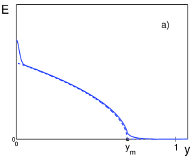
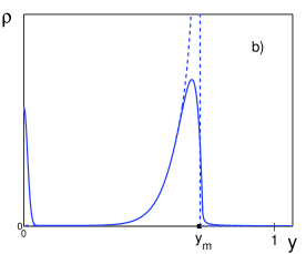
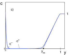
Figure 2: Schematic for limiting processes in a steady–state equilibrium: a) electric field $E{\,=\,}d\Phi/dy$; b) volume charge density $\rho{\,=\,c^{+}\,-\,}c^{-}$; c) ion concentrations $c{\,=\,}c^{+}$ and $c{\,=\,}c^{-}$. The dashed line is the outer solution in the small vicinities of $y{\,=\,}0$ (the double ion boundary layer) and $y{\,=\,}y_{m}$ (the boundary layer between the volume space charge region and the diffusion layer). The solid and dashed lines depict exact and asymptotic solutions for small $\varepsilon$.

The solution (2)–(4) describes extreme non–equilibrium over–limiting regimes, while (1) is valid for the under–limiting regimes. A unified asymptotic description of EDL valid from under–limiting to extreme non–equilibrium over–limiting regimes is developed by Zaltzman and Rubinstein [9].

Experimental evidence of the electro–convective instability. With further increase of the potential drop between the membranes, the over–limiting currents eventually arise, and steady–state equilibria lose their applicability (transition from the regime B to C in Fig. 1). In general, four physical mechanisms can be responsible for that phenomenon. Additional charge carriers due to electrolyte splitting and exaltation effects are assumed to be responsible for over–limiting currents in Belova et al. [24], Pismenskaya et al. [25]. Rayleigh–Benard convection (see review by Cross and Hohenberg  [26]) can be also due to the Ohmic heating, hence, it can provide another physical mechanism responsible for the over–limiting regimes. However, for a relatively small distance between membranes, the gravity–convection effect is absent, since the Rayleigh number $Ra$ is less than the critical value, $Ra_{cr}{\,=\,}1708$ (see experimental data in  [24], [25]). Finally, Rubinstein, Staude and Kedem [27] found experimentally that the transition to the overlimiting regime C (see Fig.  1) is accompanied by current oscillations which are regular at a small super–criticality and irregular at a large super–criticality (regimes  $C_{I}$ and  $C_{II}$ in Fig. 1). The above–mentioned facts indirectly indicate to a correlation between the instability and over–limiting currents. The correlation between the electro–convective instability and the over–limiting regimes is demonstrated in Maletzki et al. [28] and Rubinstein et al. [29], where the over–limiting regimes are eliminated when instability has been artificially suppressed. The first direct experimental proof of the electro–convective instability, which arises with increasing potential drop between the bulk ion–selective membranes, is reported by Rubinstein et al. [30], who manage to show the existence of small vortices near the membrane surface. Yossifon and Chang [11] also observe an array of electro–convective vortices arising under the effect of a slow AC electric field, while Kim et al. [31] observe non–equilibrium electroosmotic vortices.

Model of electroconvection as a stability lost of steady–state equilibria. As it was mentioned above, the over–limiting currents are accompanied by an instability of the membrane system. The following two modes of electroconvection in strong electrolytes are distinguished: i) bulk electroconvection due to the volume electric forces [32]–[39]; and ii) common electroosmosis, either of the classical “first” kind [40]–[45] or of the “second” kind [40]–[43]. In the first kind electroosmosis, a slip velocity results from the tangential electric field applied to the space charge of a quasi–equilibrium EDL [9], while in the second kind regimes, slip velocity results from the field applied to the ESC.

The stability theory of 1D quiescent steady–state EDL is developed by Rubinstein and Zaltzman [46],[47] for the extreme nonequilibrium conditions (2)–(4). First, the region $0{\,\leqslant\,y\,\leqslant\,}L$ is subdivided into the space charge, $0{\,\leqslant\,y\,<\,}y_{m}$, and electro–neutral, $y_{m}{\,<\,y\,\leqslant\,}L$, regions. The latter consists of the diffusion layer region, $y_{m}{\,<\,y\,<\,}1$, and the bulk neutral region, $1{\,<\,y\,\leqslant\,}L$. For the over–limiting regimes, the current inhomogeneity along the membrane leads to a convective motion of fluid with the tangential slip velocity, $U_{m}$, which is determined from the solution in the ESC region, $0<y\leqslant y_{m}$. Then the concentration, pressure and velocity are determined in the electro–neutral region, $y_{m}{\,<\,y\,\leqslant\,}L$, using the slip velocity found above as the boundary value at $y=y_{m}$. The 1D steady–state equilibrium solution is found to be stable for under–limiting regimes and unstable for over–limiting regimes. The corresponding marginal stability curve (in the plane of the potential drop, $\Delta\Phi$, and wave number, $\alpha$) has no upper branch, and the growth rate increases infinitely with the wave number. A regularized problem that takes into account the higher order terms in $\varepsilon$ and predicts the upper branch, is offered by Rubinstein and Zaltzman [48]. Linear stability results for various asymptotic formulations along with numerics are presented by Rubinstein, Zaltzman and Lerman [49]. Instability theory of 1D quiescent steady–state solution uniformly valid for both equilibrium and non–equilibrium conditions (not necessarily of the extreme type) is developed by Zaltzman and Rubinstein [9]. They obtain that non–equilibrium electroosmotic instability occurs at the transition from the quasi–equilibrium to the non–equilibrium EDL regime.

Note the numerical simulations of the nonlinear unsteady problem which demonstrate, in qualitative agreement with experimental data, the formation of the pair vortices and their development to chaotic motion in the electro–neutral region ([48, 50]).

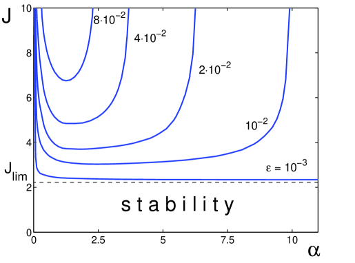
Figure 3: Marginal stability curves at different $\varepsilon$, numerics. The under–limiting regimes are stable (adopted from Demekhin et al. [10]).

New type of equilibria and their stability. Although the cells observed in Rayleigh–Benard convection and Benard–Marangoni thermo–convection look like the cells in the electro–convective motion, the latter instability is much more complicated from both physical and mathematical points of view. In particular, electro–hydrodynamics of electrolytes between membranes manifests new types of equilibria and their instabilities developed in micro– and nano–scales.

The present numerical calculations evaluate the settling time as about several minutes, while experiments demonstrate that the characteristic time for the instability to manifest itself is about several seconds (see [11], [24], [29] and the Subsection IIC). Thus, although the problem solution eventually reaches a steady–state equilibrium which becomes unstable, an unsteady solution can lose its stability long before the relaxation to the steady state. These two unperturbed solutions, steady–state and self–similar unsteady ones, are rather correspond to different, gradual and instantaneous loading of the potential drop to the membrane system, respectively.

The existence of this novel type of unsteady solutions has been recently predicted numerically for small $\varepsilon$ at intermediately long times [10] and observed experimentally [11]. In the present work, unsteady transient equilibria and their stability are investigated both asymptotically and numerically. The present asymptotic analysis is restricted by the limiting regimes and their transition to the over–limiting regimes. The results of the present asymptotic analysis are consistent with the exact numerical solution.

The paper is structured as follows. In the next Section, the governing relations are presented and typical characteristic values of the system parameters are evaluated. The 1D unsteady and 1D self–similar problems are developed for intermediately long times. Numerical justification of closeness of the exact solution of the initial–boundary problem to the solution of the self–similar problem is justified numerically for intermediately long times. In Section III, 1D explicit solutions of the self–similar problem are obtained for small Debye length and compared with the numeric solutions for intermediately long times. A two–parametric family of self–similar unsteady equilibrium solutions is found and their stability is investigated. The justification of self–similarity is done both numerically and asymptotically. In Section IV, the unsteady 2D problem is made dimensionless, and simplified equations are derived for small Debye length. Section V describes the linear stability of the 1D self–similar solutions slowly varying with time. The resulting marginal stability curves are compared with those obtained by direct numerical simulations. Some of cumbersome calculations for electrostatic solution in the space charge region and for slip velocity are in Appendixes A and B, respectively.

II. THE PHYSICAL MODEL AND
1D SELF–SIMILAR PROBLEM

A. Governing equations and typical values of parameters

Electro–convection in a binary electrolyte between semi–selective ion–exchange membranes is described by the equations for ion transport, the Poisson equation for the electric potential and the Stokes equation for a creeping flow (this model was first introduced in [9]):

$$\frac{\partial\tilde{c}^{\pm}}{\partial\tilde{t}}+\tilde{\textbf{U}}\cdot\tilde{\nabla}\tilde{c}^{\pm}=\tilde{D}\left\{\ \pm\frac{\tilde{F}}{\tilde{R}\tilde{T}}\tilde{\nabla}\cdot\left(\tilde{c}^{\pm}\tilde{\nabla}\tilde{\Phi}\right)+\tilde{\nabla}^{2}\tilde{c}^{\pm}\right\},$$ (5)

$$\tilde{\nabla}^{2}\tilde{\Phi}=\frac{\tilde{F}}{\tilde{\epsilon}}\left(\tilde{c}^{-}-\tilde{c}^{+}\right),$$ (6)

$$-\tilde{\nabla}\tilde{P}+\tilde{\mu}\tilde{\nabla}^{2}\tilde{\textbf{U}}+\tilde{F}\left(\tilde{c}^{-}-\tilde{c}^{+}\right)\tilde{\nabla}\tilde{\Phi}=0,\ \ \ \ \tilde{\nabla}\cdot\tilde{\textbf{U}}=0,$$ (7)

This system of dimensional equations is complemented by the proper initial and boundary conditions which are as follows

$$\tilde{c}^{+}=\tilde{p},\ \ \ \displaystyle-\frac{\tilde{F}\tilde{c}^{-}}{\tilde{R}\tilde{T}}\frac{\partial\tilde{\Phi}}{\partial\tilde{y}}+\frac{\partial\tilde{c}^{-}}{\partial\tilde{y}}=0,\ \ \ \tilde{\Phi}=0,\ \ \ \tilde{\textbf{U}}=0\ \ \ \mbox{for}\ \ \ \tilde{y}=0,$$ (8)

$$\tilde{c}^{+}=\tilde{p},\ \ \ \displaystyle-\frac{\tilde{F}\tilde{c}^{-}}{\tilde{R}\tilde{T}}\frac{\partial\tilde{\Phi}}{\partial\tilde{y}}+\frac{\partial\tilde{c}^{-}}{\partial\tilde{y}}=0,\ \ \ \tilde{\Phi}=\Delta\tilde{V},\ \ \ \tilde{\textbf{U}}=0\ \ \ \mbox{for}\ \ \ \tilde{y}=L,$$ (9)

$$\tilde{c}^{+}=\tilde{c}^{-}=\tilde{c}_{\infty}\ \ \ \mbox{for}\ \ \ \tilde{t}=0.$$ (10)

Here $\tilde{c}^{+},\ \tilde{c}^{-}$ are the molar concentrations of cations and anions; $\tilde{\textbf{U}}=\{\tilde{U},\>\tilde{V},\>\tilde{W}\}$ is the fluid velocity; $\{\tilde{x},\>\tilde{y},\>\tilde{z}\}$ are the coordinates, $\tilde{y}$ is normal to the membrane surface; $\tilde{\Phi}$ is the electrical potential; $\tilde{\epsilon}$ is the permittivity of the medium; $\tilde{P}$ is the pressure; $\tilde{c}_{\infty}$ is the initial ion concentration; $\tilde{F}$ is Faraday’s constant; $\tilde{R}$ is the universal gas constant; $\tilde{T}$ is an absolute temperature; $\tilde{\mu}$ is the dynamic viscosity of the fluid; $\tilde{D}$ is the cationic and anionic diffusivity; $\tilde{p}$ is the interface concentration.

It is convenient to use the characteristic electric current $\tilde{j}$ at $\tilde{y}=0$ which is related with the known total potential drop between membranes $\Delta\tilde{V}$

$$\tilde{j}=\frac{\tilde{D}\tilde{F^{2}}}{\tilde{R}\tilde{T}}\,\tilde{c}^{+}\frac{\partial\tilde{\Phi}}{\partial\tilde{y}}+\tilde{D}\tilde{F}\frac{\partial\tilde{c}^{+}}{\partial\tilde{y}},\ \ \ \ \ \ \tilde{y}=0.$$ (11)

Let us evaluate the parameters of the system. The bulk concentration of the aqueous electrolytes varies in the range $\tilde{c}_{\infty}{\,=\,1\,\div\,10^{3}\ }mol/m^{3}$; the potential drop is about $\Delta\tilde{V}{\,=\,0\,\div\,5\ }V$; the absolute temperature can be taken as $\tilde{T}{\,=\,300^{0}\ }K$; the diffusivity is about $\tilde{D}{\,=\,2\,\cdot 10^{-9}\ }m^{2}/s$; the distance between the electrodes $\tilde{L}$ is of the order of $0.5{\,\div\,}1.5$ $mm$; the concentration value $\tilde{p}$ on the membrane surface must be much higher than $\tilde{c}_{\infty}$, and it is usually taken within the range from $5\tilde{c}_{\infty}$ to $10\tilde{c}_{\infty}$ ( [3], [9], [51]). The dimensional Debye layer thickness $\tilde{\lambda}_{D}$ is varied in the range from $0.5$ to $15\ nm$ depending on the concentration $\tilde{c}_{\infty}$.

B. 1D unsteady problem at intermediately long times

Let us consider an 1D unsteady equilibrium state:

$$\tilde{\textbf{U}}=0,\qquad\frac{\partial}{\partial\tilde{x}}=\frac{\partial}{\partial\tilde{z}}=0.$$ (12)

Then the system (5)–(11) turns into

$$\frac{\partial\tilde{c}^{\pm}}{\partial\tilde{t}}=\tilde{D}\left\{\pm\frac{\tilde{F}}{\tilde{R}\tilde{T}}\frac{\partial}{\partial\tilde{y}}\left(\tilde{c}^{\pm}\frac{\partial\tilde{\Phi}}{\partial\tilde{y}}\right)+\frac{\partial^{2}\tilde{c}^{\pm}}{\partial\tilde{y}^{2}}\right\},$$ (13)

$$\frac{\partial^{2}\tilde{\Phi}}{\partial\tilde{y}^{2}}=\frac{\tilde{F}}{\tilde{\epsilon}}(\tilde{c}^{-}-\tilde{c}^{+}),$$ (14)

$$\tilde{c}^{+}=\tilde{p},\ \ \ \displaystyle-\frac{\tilde{F}\tilde{c}^{-}}{\tilde{R}\tilde{T}}\frac{\partial\tilde{\Phi}}{\partial\tilde{y}}+\frac{\partial\tilde{c}^{-}}{\partial\tilde{y}}=0,\ \ \ \ \ \tilde{\Phi}=0\ \ \ \mbox{for}\ \ \ \tilde{y}=0,$$ (15)

$$\tilde{c}^{+}=\tilde{p},\ \ \ \displaystyle-\frac{\tilde{F}\tilde{c}^{-}}{\tilde{R}\tilde{T}}\frac{\partial\tilde{\Phi}}{\partial\tilde{y}}+\frac{\partial\tilde{c}^{-}}{\partial\tilde{y}}=0,\ \ \ \ \ \tilde{\Phi}=\Delta\tilde{V}\ \ \ \mbox{for}\ \ \ \tilde{y}=\tilde{L},$$ (16)

$$\tilde{c}^{+}=\tilde{c}^{-}=\tilde{c}_{\infty}\ \ \ \mbox{for}\ \ \ \tilde{t}=0,$$ (17)

$$\tilde{j}=\frac{\tilde{D}\tilde{F^{2}}}{\tilde{R}\tilde{T}}\,\tilde{c}^{+}\frac{\partial\tilde{\Phi}}{\partial\tilde{y}}+\tilde{D}\tilde{F}\frac{\partial\tilde{c}^{+}}{\partial\tilde{y}},\ \ \ \tilde{y}=0.$$ (18)

According to (13)–(18), at $\Delta\tilde{V}=0$, a neutral steady–state solution with a uniform concentration of ions, $\tilde{c}^{+}{\,=\,\tilde{c}^{-}=\,}\tilde{c}_{\infty}$, instantaneously loses its equilibrium under the effect of the potential drop, $\Delta\tilde{V}$, applied at $\tilde{t}{\,=\,}0$ and kept constant at $\tilde{t}{\,>\,}0$. As a result, a concentration polarization of ions is formed in thin boundary layers near the membrane surfaces, which expand with time. After several milliseconds of evolution, the diffusion layer thickness, $\tilde{\delta}$, will be much larger than the Debye length, $\tilde{\lambda}_{D}{\,=\,}(\tilde{\epsilon}\tilde{R}\tilde{T}/\tilde{c}_{\infty})^{1/2}/\tilde{F}$, $\quad\tilde{\delta}(\tilde{t})\gg\tilde{\lambda}_{D}.$ On the other hand, there is a wide interval of time $\tilde{t}$ (from seconds to minutes), such that $\tilde{\delta}(\tilde{t})\ll\tilde{L}$:

$$\tilde{\lambda}_{D}\ll\tilde{\delta}(\tilde{t})\ll\tilde{L}.$$ (19)

We assume that the diffusion–layer thickness $\tilde{\delta}(\tilde{t})$ in the 1D unsteady solution varies in time as

$$\tilde{\delta}(\tilde{t})=2\sqrt{\tilde{D}\tilde{t}}.$$ (20)

Then (19) can be presented in the form

$$\frac{\tilde{\lambda}_{D}^{2}}{4\tilde{D}}\ll\tilde{t}\ll\frac{\tilde{L}^{2}}{4\tilde{D}}.$$ (21)

Let us study the problem for intermediately long times which belong to the interval (21). The spatial structure of the unsteady limiting regimes at any fixed time is qualitatively similar to that of the steady–state equilibria depicted in Fig. 2. The space between the membranes can be divided into the following regions of inhomogeneity: (I) a thin EDL near the membrane surface $\tilde{y}{\,=\,}0$; ESC region (II) separated from the diffusion layer (III) by a thin internal boundary layer (IV); a bulk neutral region (V).

For unsteady solutions, the influence of the upper membrane $\tilde{y}{\,=\,}\tilde{L}$ is neglegible within the interval (21), and the boundary conditions (16) should be revised. Subtracting the second equation (13) for $\tilde{c}^{-}$ from the first equation (13) for $\tilde{c}^{+}$, integrating the result from $0$ to some $\tilde{y}$ within the bulk neutral region, and neglecting the higher order terms with respect to small $\tilde{\delta}/\tilde{L}$, the known linear voltage distribution in the bulk neutral region is obtained

$$\tilde{\Phi}(\tilde{y})\sim const+\frac{\tilde{j}\tilde{R}\tilde{T}}{2\tilde{F}^{2}\tilde{D}\tilde{c}_{\infty}}\,\tilde{y},\ \ \ \tilde{y}\gg\tilde{\delta}.$$ (22)

Here the $constant$ and the electric current $\tilde{j}$ are functions of time. The relation (22) predicts unbounded linear behavior of the potential at a large distance from the bottom membrane. This infers the following effective boundary condition at large $y$

$$\lim_{\tilde{y}/\tilde{\delta}\rightarrow\infty}\left(\tilde{\Phi}-\frac{\tilde{j}\tilde{R}\tilde{T}}{2\tilde{F}^{2}\tilde{D}\tilde{c}_{\infty}}\,\tilde{y}\right)=\Delta\tilde{\Phi},$$ (23)

which, along with the following condition for the concentrations

$$\lim_{\tilde{y}/\tilde{\delta}\rightarrow\infty}\tilde{c}^{+}=\lim_{\tilde{y}/\tilde{\delta}\rightarrow\infty}\tilde{c}^{-}=\tilde{c}_{\infty}$$ (24)

substitute the BC’s (16) for the problem with the distance between the upper and bottom membranes that satisfies (19). Note that Ohmic current is taken into account due to a cumulative effect at a large distance from the membrane.

Introducing a similar effective voltage instead of the total voltage $\Delta V$ is useful also for the finite membrane problem both for the efficiency of calculations and comparison with the case of the distant upper membrane:

$$\Delta\tilde{\Phi}=\Delta\tilde{V}-\frac{\tilde{j}\tilde{R}\tilde{T}\tilde{L}}{2\tilde{F}^{2}\tilde{D}\tilde{c}_{\infty}}.$$ (25)

In fact, the effective voltage $\Delta\tilde{\Phi}$ in the EDL and ESC regions does not depend on the distance between the membranes.

The formulated problem does not contain a characteristic length, since neither the distance between the electrodes nor the double–ion length can give such a scale within the interval (21). This infers the solution self–similarity [52] with the diffusion layer thickness as the dynamic characteristic size ( justification of self–similarity in small $\varepsilon$ see in Section II.C). Let us transform the problem into a dimensionless form using the characteristic values of potential, $\displaystyle\tilde{\Phi}_{0}{\,=\,}\tilde{R}\tilde{T}/\tilde{F}$, concentration, $\tilde{c}_{\infty}$, and time, $\tilde{t}_{0}$, by introducing the following new independent variables:

$${\tau}={t},\ \ \ \ \eta=\frac{\tilde{y}}{\tilde{\delta}(\tilde{t})}.\,\,$$ (26)

This gives

$$\begin{array}[]{c}\displaystyle\frac{\partial c^{+}}{\partial\tau}=2\eta\frac{\partial c^{+}}{\partial\eta}+\frac{\partial}{\partial\eta}\left(c^{+}\frac{\partial\Phi}{\partial\eta}\right)+\frac{\partial^{2}c^{+}}{\partial\eta^{2}},\\[14.0pt] \displaystyle\frac{\partial c^{-}}{\partial\tau}=2\eta\frac{\partial c^{-}}{\partial\eta}-\frac{\partial}{\partial\eta}\left(c^{-}\frac{\partial\Phi}{\partial\eta}\right)+\frac{\partial^{2}c^{-}}{\partial\eta^{2}},\\[14.0pt] \displaystyle\varepsilon^{2}\frac{\partial^{2}\Phi}{\partial\eta^{2}}=c^{-}-c^{+},\\ \end{array}$$ (27)

where $\displaystyle\varepsilon{\,=\,}\tilde{\lambda}_{D}/\tilde{\delta}(\tilde{t})$.

Assume now that for intermediately long times the solution, indeed, becomes self–similar (see Section II.C), i. e.

$$\begin{array}[]{c}\displaystyle 2\eta\frac{dc^{+}}{d\eta}+\frac{d}{d\eta}\left(c^{+}E+\frac{dc^{+}}{d\eta}\right)=0,\\[14.0pt] \displaystyle 2\eta\frac{dc^{-}}{d\eta}+\frac{d}{d\eta}\left(-c^{-}E+\frac{dc^{-}}{d\eta}\right)=0,\\[14.0pt] \displaystyle\varepsilon^{2}\frac{dE}{d\eta}=c^{-}-c^{+},\end{array}$$ (28)

with the BC’s

$$\begin{array}[]{cc}&\ \ \ c^{+}=p,\ \ \ \displaystyle c^{-}E-\frac{dc^{-}}{d\eta}=0,\ \ \ \Phi=0\ \ \ \mbox{for}\ \ \ \eta=0,\end{array}$$ (29)

$$\begin{array}[]{cc}&\ \ \ \displaystyle c^{-}\to 1,\ \ \ c^{+}\to 1,\ \ \ \displaystyle\Phi-\frac{J\eta}{2}\to\Delta\Phi\ \ \ \mbox{at}\ \ \ \eta\to\infty.\end{array}$$ (30)

Here $\displaystyle E{=\,}\frac{d\Phi}{d\eta}$, $\Delta\Phi{\,=\,}\Delta\tilde{\Phi}/\tilde{\Phi}_{0}$, the dimensionless electric current at $\eta=0$ is determined by

$$J=c^{+}E+\frac{dc^{+}}{d\eta},\ \ \ \eta=0.$$ (31)

Solutions of the self–similar boundary problem (28)–(31) are presented in Fig. 4 for the charge distribution $\rho(\eta){\,=\,c^{+}(\eta)\,-\,}c^{-}(\eta)$ and positive ions concentration $c^{+}(\eta)$ for different values of the parameters. Voltage–current characteristics $J$ versus $\Delta\Phi$ for different $\varepsilon$ are shown in Fig. 5 for both the exact numeric and asymptotic self–similar solutions.

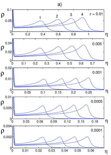
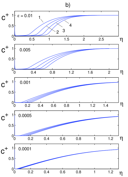
Figure 4: Self–similar charge $\rho=c^{+}-c^{-}$ (a) and concentration $c^{+}$ distribution (b) for different $\varepsilon$. Curves correspond to the following values of electric potential drop: 1. $\Delta\Phi=50$; 2. $\Delta\Phi=100$; 3. $\Delta\Phi=150$; 4. $\Delta\Phi=200$.

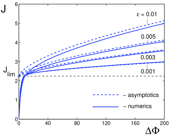
Figure 5: VC curves. Comparison of the self–similar asymptotics (dashed lines) and the exact numerics (solid lines) for several $\varepsilon$.

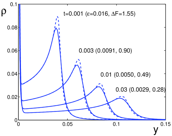
Figure 6: Distribution of the charge density $\rho$ in space for several moments of time, $\Delta V=100$ and $\nu{\,=\,}\tilde{\lambda}_{D}/\tilde{L}=0.001$. Solid line corresponds to the numerical solution of the unsteady problem (32)–(36). Two–parametric self–similar solution of (28)–(31) with $\varepsilon$ and $\Delta\Phi$ parametrically changing with time is depicted by dashed lines.

C. Numerical justification of the self–similar problem

To justify self–similarity of the solution of (28)–(31) for intermediately long times, we compare it with the exact numerical solution of the initially–boundary problem (13)–(18). In this numeric simulations, the time $\tilde{t}$ and the coordinate $\tilde{y}$ are referred to $\tilde{L}^{2}/\tilde{D}$ and $\tilde{L}$. The concentrations $\tilde{c}^{\pm}$ and the potential $\tilde{\Phi}$ are referred to $\tilde{c}_{\infty}$ and $\tilde{\Phi}_{0}$, respectively, as it was done for the self–similar solution. The system (13)–(18) turns into

$$\frac{\partial c^{\pm}}{\partial t}=\pm\frac{\partial}{\partial y}\left(c^{\pm}\frac{\partial\Phi}{\partial y}\right)+\frac{\partial^{2}c^{\pm}}{\partial y^{2}},$$ (32)

$$\nu^{2}\frac{\partial^{2}\Phi}{\partial y^{2}}=c^{-}-c^{+},$$ (33)

$$c^{+}=p,\ \ \ \displaystyle-c^{-}\frac{\partial\Phi}{\partial y}+\frac{\partial c^{-}}{\partial y}=0,\ \ \ \Phi=0\ \ \ \mbox{for}\ \ \ y=0,$$ (34)

$$c^{+}=p,\ \ \ \displaystyle-c^{-}\frac{\partial\Phi}{\partial y}+\frac{\partial c^{-}}{\partial y}=0,\ \ \ \Phi=\Delta V\ \ \ \mbox{for}\ \ \ y=1,$$ (35)

$$c^{+}=c^{-}=1,\ \ \ \displaystyle\mbox{for}\ \ \ t=0,$$ (36)

$$j=\,c^{+}\frac{\partial\Phi}{\partial y}+\frac{\partial c^{+}}{\partial y},\ \ \ y=0,$$ (37)

where $\nu{\,=\,}\tilde{\lambda}_{D}/\tilde{L}$, $\Delta V{\,=\,}\Delta\tilde{V}/\tilde{\Phi}_{0}$, $j{\,=\,}\tilde{j}\tilde{L}/(\tilde{D}\tilde{F}\tilde{c}_{\infty})$.

The system (32)–(37) is integrated numerically using Gear’s method in time along with Galerkin’s $\tau$–method digitization with respect to the space variable. The problem is described by two parameters, the voltage between membranes, $\Delta V$, and analog of $\varepsilon$ in a finite size system, $\nu\ll 1$. The calculations are fulfilled for the limiting regimes, $\nu$ and $\Delta V$ are varied in the ranges $\nu{\,=\,}0.00001\div 0.01$ and $\Delta V{\,=\,}50\div 200$. It is found numerically that the solution reaches the steady–state equilibrium at $t_{s}{\,=\,0.1\,\div\,}0.2$. Taking characteristic values $\tilde{D}{\,=\,2\,\cdot 10^{-9}\ }m^{2}/s$ and $\tilde{L}=$ $0.5{\,\div\,}1.5$ $mm$, this time is evaluated in a dimensional form as $\tilde{t}_{s}=$ $0.25{\,\div\,}4$ $min$, supporting the assumption in Subsection AI. Below, we restrict ourselves by the regimes satisfying the inequality (21) which can be generalized now as

$$\frac{\nu^{2}}{4}\ll t\ll t_{s}.$$ (38)

The two–parametric family of self–similar solutions of the problem (28)–(31) is calculated for a wide range of the parameters $\Delta\Phi$ and $\varepsilon$ and accumulated for further comparison with the exact numerical solution for the finite–length membrane geometry. For the comparison of the self–similar solution with the exact numerical solution for the finite–length membrane geometry, the parameters $\Delta\Phi$ and $\varepsilon$ varying with time are calculated using relations

$$\varepsilon(t)=\frac{\nu}{2\sqrt{t}},\quad J(t)=2j(t)\sqrt{t},\quad\Delta\Phi(t)=\Delta V-\frac{j(t)}{2}.$$ (39)

Here the Ohmic voltage, $j(t)/2$, is excluded from the total voltage $\Delta V$. These values are substituted into the accumulated family of self–similar solutions (28)–(31) obtained previously for a wide range of the two values $\Delta\Phi$ and $\varepsilon$.

The charge density $\rho{\,=\,c^{+}\,-\,}c^{-}$ is presented in Fig. 6 for both exact and approximate self–similar solutions. The unsteady solution is “adiabatically” sliding along the two–parametric self–similar solution, $\Delta\Phi(t)$ and $\varepsilon(t)$. One can see a rather good correspondence between these two solutions for intermediately long times.

This expands the applicability of the approach up to quite realistic values of the potential drop. Thus, the present asymptotic model is applied to the dimensionless potential drop $0<\Delta\Phi<200$ (which corresponds to dimensional values $0\div 5V$). The asymptotic model describes the limiting regimes with the error value depending on $\varepsilon$. For $\varepsilon=0.01$ and $\Delta\Phi=40$ the error is about $20\%$, while for $\Delta\Phi=200$ and the same $\varepsilon=0.01$ it is about $3\%$. For $\varepsilon=0.001$ the error is much smaller, for example for $\Delta\Phi=20$ it is about $1\%$ and for $\Delta\Phi=200$ less than $0.2\%$.

For the self–similar solution the diffusion layer thickness should be inversely proportional to the electric current, $\delta(t)\sim 1/j(t)\sim\sqrt{t}$. Typical evolution of $1/j(t)$ presented in Fig. 7 exhibits three characteristic time intervals. In the interval $II$, for the intermediately long times (38), $1/j(t)$ is proportional to $\sqrt{t}$ and the assumption (20) is satisfied, while for short times, in the time interval $I$, as well as for long times, in the interval $III$, the self–similarity is violated.

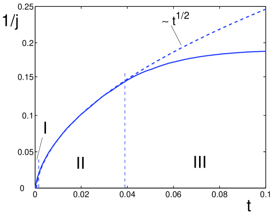
Figure 7: Typical evolution of $1/j(t)$. I is the short–time region of influence of the initial data; II is the intermediately–long–time region of self–similarity, and III is the region of influence of the upper membrane $y{\,=\,}1$, ($\Delta V{\,=\,}100$ and $\nu{\,=\,}\tilde{\lambda}_{D}/\tilde{L}{\,=\,}0.001$).

III. 1D SELF–SIMILAR SOLUTIONS FOR
SMALL DIMENSIONLESS DEBYE LENGTH

A. 1D explicit solutions

To find 1D self–similar equilibrium solutions explicitly, we apply to (28)–(31) the asymptotic decomposition method widely used for 1D steady–state equilibria at small $\varepsilon$, [14]–[21]. The reduced problem allows a relatively simple solution for the electric field, which consists of two branches on the left and right of the boundary of the space–charge region $\eta{\,=\,}\eta_{m}$. The value $\eta_{m}$ is determined by the solution of the problem. The resulting outer solution is weakly singular at $\eta{\,=\,}\eta_{m}$, where the electric field gradient has a discontinuity. This procedure ignores the EDL near the membrane surface $\eta{\,=\,}0$ (the first boundary condition $c^{+}=p$ in (29) is rejected), but predicts the existence and location of the internal boundary layer in the vicinity of $\eta{\,=\,}\eta_{m}$. The influence of these boundary layers on the limiting regimes is negligibly small for vanishing $\varepsilon$. In particular, the potential drop within these boundary layers is much less by the order in $\varepsilon$ than that within the ESC region. As in the steady–state case, the matching conditions of the outer solution with the inner ones within the boundary layers are substituted by the patching conditions. Such a description, in spite of its simplicity, well describes solutions of both equilibrium and stability problems as demonstrated below by their comparison with numerics. Within the adopted asymptotic approach, the interface elevation $\eta{\,=\,}\eta_{m}$ is a new natural variable inherent to the problem. It first arises explicitly in the equilibrium solution as the boundary between the extended space charge region and the region of the diffusion layer, in which the equilibrium states are described separately by the outer solution. Then the stability study employs perturbation of the interface elevation $\eta_{m}$ along with the perturbations of all conventional variables such as concentrations, velocity etc. Hence, the system development is accompanied by the interface instability, which reflects the physical nature of the system.

Following the decomposition method to leading order in $\varepsilon$, the new scaled variables $F$ and $\Gamma$ are introduced for the equilibrium problem:

$$F=\varepsilon\left(\Phi-\frac{J\eta}{2}\right),\ \ \ \Gamma=c^{+}+c^{-}-\frac{1}{2}H^{2},\ \ \ \Delta F=\varepsilon\Delta\Phi,\ \ \ H=\frac{dF}{d\eta}.$$ (40)

Substituting (40) into (28)–(31) yields after some algebra:

$$\frac{d^{2}\Gamma}{d\eta^{2}}=-2\eta\frac{d}{d\eta}\left(\Gamma+\frac{1}{2}H^{2}\right),$$ (41)

$$\frac{d}{d\eta}\left[\left(\Gamma+\frac{1}{2}H^{2}\right)H\right]=0,$$ (42)

$$\left(\Gamma+\frac{1}{2}H^{2}\right)H=0,\ \ \ F=0\ \ \ \mbox{for}\ \ \ \eta=0,$$ (43)

$$\Gamma+\frac{1}{2}H^{2}\to 2,\ \ \ F\to\Delta F\ \ \ \mbox{at}\ \ \ \eta\to\infty,$$ (44)

and the auxiliary condition for the electric current $J$ related to $\Gamma$

$$J=\frac{d\Gamma}{d\eta},\ \ \ \eta=0.$$ (45)

To completely determine the outer solution in variables $F$, $H$ and $\Gamma$, first the patching condition of the outer solutions is applied to the function $(\Gamma+H^{2})H$ at $\eta{\,=\,}\eta_{m}$, ignoring the input of the internal boundary layer at $\eta{\,=\,}\eta_{m}$. Note also that the method of decomposition ignores the input of the boundary layer in $\eta=0$ into the outer region, and the boundary condition (29) for $c^{+}$ at $\eta=0$ is rejected. Then equations (42) and the first of equations (43) yield

$$\left(\Gamma+\frac{1}{2}H^{2}\right)H=0.$$ (46)

Equation (46) yields the outer solution separately in the space–charge, $0\leqslant\eta\leqslant\eta_{m}$, and electro–neutral, $\eta\geqslant\eta_{m}$, regions:

$$\Gamma+\frac{1}{2}H^{2}=0\ \ \ \mbox{for}\ \ \ 0\leqslant\eta<\eta_{m},$$ (47)

$$H=0\ \ \ \mbox{for}\ \ \ \eta>\eta_{m}.$$ (48)

Then, using equations (47)–(48), conditions of continuity for $F$, $H$, $\Gamma$ and $d\Gamma/d\eta$ and the rest of equations (41)–(45) lead to the following relations in the space–charge, and electro–neutral regions:

$$\Gamma=J\left(\eta-\eta_{m}\right),\ \ \ F=\Delta F\left[1-\left(1-\frac{\eta}{\eta_{m}}\right)^{3/2}\right]\ \ \ \mbox{for}\ \ \ 0\leqslant\eta<\eta_{m},$$ (49)

$$\Gamma=2-2\frac{\mbox{erfc}(\eta)}{\mbox{erfc}(\eta_{m})},\ \ \ F=\Delta F\equiv const\ \ \ \mbox{for}\ \ \ \eta>\eta_{m}.$$ (50)

Returning to the old variables, $c^{+}$, $c^{-}$, $H$ and $\rho$, we obtain

$$c^{+}=c^{-}=0,\ \ \ H=\sqrt{2J\left(\eta_{m}-\eta\right)},\ \ \ \rho=\varepsilon\sqrt{\frac{J}{2(\eta_{m}-\eta)}}\ \ \ \mbox{for}\ \ \ 0\leqslant\eta<\eta_{m},$$

$$c^{+}=c^{-}=1-\frac{\mbox{erfc}(\eta)}{\mbox{erfc}(\eta_{m})},\ \ \ H=0,\ \ \ \rho\equiv 0\ \ \ \mbox{for}\ \ \ \eta>\eta_{m}.$$

Here, to the leading order in $\varepsilon$, the volume charge in space–charge region has a singularity at $\eta{\,=\,}\eta_{m}$. To overcome this inhomogeneity of the outer solution (49)–(50) in the vicinity of $\eta{\,=\,}\eta_{m}$, the inner solution should be developed.

According to this solution the potential drop in space–charge region is approximately equal to the total voltage between the membranes:

$$\Delta F=\varepsilon\Delta\Phi\approx\varepsilon\Delta V.$$ (51)

The values $\Delta F$ and $J$ are interrelated:

$$\Delta F=\sqrt{\frac{8}{9}J}\,\eta_{m}^{3/2},$$ (52)

with the relation between $\eta_{m}$ and current $J$

$$J=\frac{4}{\sqrt{\pi}}\frac{\exp{(-\eta_{m}^{2})}}{\mbox{erfc}\left(\eta_{m}\right)}.$$ (53)

Relations (52) and (53) determine implicitly the V–C curve and the boundary of the ESP region $\eta_{m}$ versus potential drop $\Delta F$

$$J\,\mbox{erfc}\left[\left(\frac{9\Delta F^{2}}{8J}\right)^{1/3}\right]=J_{lim}\exp\left[-\left(\frac{9\Delta F^{2}}{8J}\right)^{2/3}\right],\ \ \ J_{lim}=\frac{4}{\sqrt{\pi}}.$$ (54)

$$\frac{9\sqrt{\pi}}{32}\Delta F^{2}=\frac{\eta_{m}^{3}\exp\left(-\eta_{m}^{2}\right)}{\mbox{erfc}\left(\eta_{m}\right)},$$ (55)

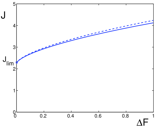
Figure 8: VC curves. Solid line relates to (54), while dashed line – to the simplified version (58).

In the subsequent stability study of the self–similar regimes, the scaled value of the potential drop is assumed to be small:

$$\Delta F\equiv\varepsilon\Delta\Phi\approx\varepsilon\Delta V\ll 1.$$ (56)

In that limit relations (54)–(55) are reduced as follows:

$$J\approx J_{lim}\left(1+\frac{2\eta_{m}}{\sqrt{\pi}}\right),\ \ \ \eta_{m}\approx\frac{\pi}{8}\left(J-J_{lim}\right),$$ (57)

$$(\Delta F)^{2}=\frac{\pi^{3}}{576}\left(J-J_{lim}\right)^{3}J.\ \ \ \$$ (58)

Evidently, (57)–(58) correspond to near–critical currents. On the other hand the analysis of the inner solution at $\eta=\eta_{m}$, and of the next order in $\varepsilon$ terms in the outer solution at $\eta>\eta_{m}$ yields that the approximate solution (49)–(50) homogeneously satisfies the condition (51) of the potential drop domination in space–charge region if

$$\varepsilon\ln\varepsilon^{-1}\ll\Delta F\ll 1.$$ (59)

Then relations (56)–(59) gives for a small potential drop:

$$\varepsilon\ln\varepsilon^{-1}\ll\eta_{m}^{3/2}\sim(J-J_{lim})^{3/2}\sim\Delta F\ll 1,\,\,\,\,J_{lim}=O((\Delta F)^{0}).$$ (60)

For a small potential drop, relations (49) and (50) yield within space–charge region:

$$c^{+}=c^{-}=0,\ \ \ F\sim\Delta F\ \ \ \Gamma\sim(\Delta F)^{2/3},\ \ \ H\sim(\Delta F)^{1/3},\ \ \ \rho\sim(\Delta F)^{-1/3},$$ (61)

and electro–neutral region:

$$c^{+}\sim c^{-}\sim(\Delta F)^{0},\ \ \ F\sim\Delta F,\ \ \ \Gamma\sim(\Delta F)^{0},\ \ \ H=0,\ \ \ \rho=0.$$ (62)

while according to equation (60), the boundary between these two regions is given by

$$(\varepsilon\ln\varepsilon^{-1})^{2/3}\ll\eta_{m}\sim(\Delta F)^{2/3}\ll 1.$$ (63)

B. Comparison of 1D explicit asymptotic and numeric solutions

In Fig. 5 the asymptotic solution for V–C curves (54) is presented as a dependence $J$ versus $\Delta\Phi$ (dashed lines) and compared with those (solid lines) obtained numerically in Subsection II.C. The comparison demonstrates a fair correspondence between the self–similar asymptotics and exact numerical solution except the region of under–limiting currents. The difference tends to zero as $\varepsilon\to 0$ e.g. at $\varepsilon=0.001$ the exact solution and asymptotics coincide with graphic accuracy. This justifies the neglect of the EDL inputs into the limiting solutions accepted in the present study.

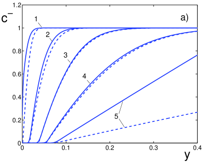
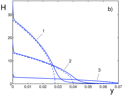
Figure 9: Negative ion concentration (a), $c^{-}$, and electric field (b), $H$, vs $y$ for several moments of time. Comparison of numerics (13)–(18) (solid lines) with self–similar asymptotics (49)–(50) (dashed lines) for (a) $\Delta V{\,=\,}50$, $\nu{\,=\,}0.001$: 1. $t{\,=\,}0.0001$; 2. $t{\,=\,}0.001$; 3. $t{\,=\,}0.004$; 4. $t{\,=\,}0.015$; 5. $t{\,=\,}0.5$; and (b) $\Delta V{\,=\,}100$, $\nu{\,=\,}0.0005$: 1. $t{\,=\,}0.001$; 2. $t{\,=\,}0.003$; 3. $t{\,=\,}0.03$.

In Fig. 8 the universal voltage–current characteristic described by (54) is plotted by solid lines, while simplified version of the VC curve (58) is plotted by dashed lines. It is seen that the difference between these two curves is extremely small for low values of $\Delta F$ and does not exceed $4\%$ at $\Delta F=1$.

In Fig. 9 the distributions of the negative ion concentration $c^{-}$ and electric field $H=\varepsilon E$ obtained from the numerical solution of (32)–(36) are shown for several $t$. In turn, in Fig. 9b self–similar distributions described by (49)–(50) are given. Except for short and long times, a rather good correspondence is observed of the both approaches at intermediately long times. In accordance to (63), the value of $\eta_{m}$, indeed, is a small value for parameters adopted in Fig. 9, where $\eta_{m}$ is determined by the condition that $\eta>\eta_{m}$ correspond to positive values of $c^{-}$.

Figure 10: Comparison of the V–C characteristics for self–similar solution and numerics, $\Delta V=50,\nu=0.00005$. Numerics (13)–(18) is shown by squares and the universal self–similar VC curve (54) – by solid line. The region of the solution self–similarity $t_{1}{\,<\,t\,<\,}t_{2}$, $t_{1}\gg\nu^{2}/4$, $t_{2}\ll t_{s}=\tilde{L}^{2}/(4\tilde{D})$. Arrows depict the time growth along the voltage–current curve.

The self–similar character of the solution for intermediately long times is illustrated in Fig. 10. In this calculation $\Delta V{\,=\,}50,\nu{\,=\,}0.00005$ are kept constant during numerical integration of the system (32)–(36). Also, the potential drop between the membrane is kept constant, its fraction $\Delta\Phi{\,=\,}\Delta V-j(t)/2$ is changing in time as well as $J$. It is clearly seen that the numerical solution follows the self–similar equilibrium. This fitting persists up to the moment $t{\,=\,}t_{2}$, when the influence of the upper membrane becomes significant.

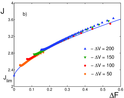
Figure 11: Numerical points for several values of the potential drop between the membranes, $\Delta V$, shrink into the universal VC curve $J(\Delta F)$ given by (54); a) $\nu{\,=\,}0.001$, b) $\nu{\,=\,}0.0005$.

The data for several $\Delta V$ are gathered in Fig. 11a) and 11b) for $\nu=0.001$ and $\nu{\,=\,}0.0005$. The data for short times $t{\,<\,}t_{1}$ and for long times $t{\,>\,}t_{2}$ are discarded from the consideration and only data for intermediately long times are kept. The numerical points for all $\Delta V$ and $\nu$ shrink into the universal VC curve, $J(\Delta F)$, described by (54). It is seen that the fitting is better for smaller $\nu$ and $\Delta V$.

IV. 2D UNSTEADY PROBLEM FOR SMALL DIMENSIONLESS DEBYE LENGTH

A. Governing relations. Dimensionless variables

Aiming at a stability study of the 1D equilibrium self–similar solutions, the 2D unsteady problem is rewritten using self–similar variables. First, the characteristic length scales, $\tilde{l}_{0}$ and $\tilde{\delta}$, tangential and normal to the membrane surface are introduced together with the characteristic scales for stream function, velocity components, pressure and electric potential as follows:

$$\tilde{l}_{0}=\frac{1}{\tilde{\alpha}},\ \ \ \tilde{\delta}=2\sqrt{\tilde{D}\tilde{t}},\ \ \ \tilde{\Psi}_{0}=\frac{\tilde{D}\tilde{\delta}}{\tilde{l}_{0}},\ \ \ \tilde{U}_{0}=\frac{\tilde{D}}{\tilde{l}_{0}},\ \ \ \tilde{V}_{0}=\frac{\tilde{D}\tilde{\delta}}{\tilde{l}_{0}^{2}},\ \ \ \tilde{P}_{0}=\frac{\tilde{\mu}\tilde{D}}{\tilde{\delta}^{2}},\ \ \ \tilde{\Phi}_{0}=\frac{\tilde{R}\tilde{T}}{\tilde{F}}.$$ (64)

The characteristic time scale, $\tilde{t}_{0}$, is also introduced as an arbitrary moderately long time at which the equilibrium solution is already settled on the self–similar regime and yet does not leave it; $\tilde{\delta}(\tilde{t})$ is the diffusion layer thickness, while $\tilde{\alpha}$ is the characteristic wave number. Preserving the same notations for dimensionless stream function, velocities and pressure as for their dimensional values, the following independent self–similar variables are introduced for the 2D problem:

$$\tau=\frac{\tilde{t}}{\tilde{t}_{0}},\ \ \ x=\frac{\tilde{x}}{\tilde{l}_{0}},\ \ \eta=\frac{\tilde{y}}{\tilde{\delta}(\tilde{t})}.\ \ \ \$$ (65)

Then the time–dependent wave number and Debye length are introduced for further convenience

$$\alpha(\tau)=\tilde{\delta}(\tilde{t})\tilde{\alpha},\ \ \ \varepsilon(\tau)=\frac{\tilde{\lambda}_{D}}{\tilde{\delta}(\tilde{t})}.$$ (66)

Functions $\alpha(\tau)$, $\varepsilon(\tau)$, characterizing the time variation of the equilibrium solution, are assumed to be slowly varied in the fast–time scale of perturbations.

Nonlinear 2D problem may be written in the following form:

$$\frac{DK}{D\tau}=\nabla\cdot(\rho\nabla\Phi)+\nabla^{2}K,$$ (67)

$$\frac{D\rho}{D\tau}=\nabla\cdot(K\nabla\Phi)+\nabla^{2}\rho,$$ (68)

$$\varepsilon^{2}\nabla^{2}\Phi=-\rho,$$ (69)

$$\nabla^{4}\Psi=-\frac{\varkappa}{\varepsilon^{2}}\nabla^{\prime}\times(\rho\nabla^{\prime}\Phi),$$ (70)

Here

$$\nabla=\left(\alpha\frac{\partial}{\partial x},\ \frac{\partial}{\partial\eta}\right),\ \ \ \nabla^{\prime}=\left(\frac{\partial}{\partial x},\ \frac{\partial}{\partial\eta}\right),\ \ \ \frac{D}{D\tau}=4\tau\frac{\partial}{\partial\tau}-2\eta\frac{\partial}{\partial\eta}+\alpha^{2}\left(U\frac{\partial}{\partial x}+V\frac{\partial}{\partial\eta}\right),$$

$K=c^{+}+c^{-}$, $\rho=c^{+}-c^{-}$ as previously in 1D problem, $\varkappa=\tilde{\epsilon}\tilde{\Phi}_{0}^{2}/(\tilde{\mu}\tilde{D})$ describes physical properties of the liquid and electrolyte; $\Psi$ is the stream function:

$$U=\frac{\partial\Psi}{\partial\eta},\ \ \ V=-\frac{\partial\Psi}{\partial x}.$$ (71)

Assuming the problem self–similarity, the following boundary conditions are accepted:

$$\Phi=0,\displaystyle\ \ \ (K-\rho)\frac{\partial\Phi}{\partial\eta}-\frac{\partial K}{\partial\eta}+\frac{\partial\rho}{\partial\eta}=0,\ \ \ K+\rho=2p,\ \ \ \Psi=\frac{\partial\Psi}{\partial\eta}=0\ \ \ \mbox{for}\ \ \eta=0,$$ (72)

$$\Phi-\frac{J\eta}{2}\to\Delta\Phi,\displaystyle\ \ \ \rho\to 0,\ \ \ K\to 2,\ \ \ \Psi\to 0,\ \ \ \frac{\partial\Psi}{\partial\eta}\to 0\ \ \ \mbox{at}\ \ \ \eta\to\infty,$$ (73)

where $J$ is the electric current (31).

B. Decomposition method for 2D problem. Ad–hoc model

Extending the decomposition method for the limiting and over–limiting regimes from 1D case to 2D case, the following auxiliary variables scaled in $\varepsilon$ are introduced:

$$F=\varepsilon\left(\Phi-\frac{J\eta}{2}\right),\ \ \ H=\frac{\partial F}{\partial\eta},\ \ \ \Gamma=K-\frac{1}{2}H^{2},\ \ \ \rho=-\varepsilon\left(\frac{\partial H}{\partial\eta}+\alpha^{2}\frac{\partial^{2}F}{\partial x^{2}}\right).$$ (74)

First the system (67)–(70) is rewritten in the variables (74) substituting $\rho=-\varepsilon\nabla^{2}F$:

$$\frac{DK}{D\tau}=-\nabla\cdot[(\nabla^{2}F)\nabla F]+\nabla^{2}K,$$ (75)

$$\varepsilon^{2}\frac{D(\nabla^{2}F)}{D\tau}=-\nabla\cdot(K\nabla F)+\varepsilon^{2}\nabla^{4}F,$$ (76)

$$\nabla^{4}\Psi=\frac{\varkappa}{\varepsilon^{2}}\nabla^{\prime}\times[(\nabla^{2}F)\nabla^{\prime}F],$$ (77)

and then substituting $K=\Gamma+\frac{1}{2}H^{2}$

$$\frac{D(\Gamma+\frac{1}{2}H^{2})}{D\tau}=-\nabla\cdot[(\nabla^{2}F)\nabla F]+\nabla^{2}\left(\Gamma+\frac{1}{2}H^{2}\right),$$ (78)

$$\varepsilon^{2}\frac{D(\nabla^{2}F)}{D\tau}=-\nabla\cdot\left[\left(\Gamma+\frac{1}{2}H^{2}\right)\nabla F\right]+\varepsilon^{2}\nabla^{4}F.$$ (79)

The following ad–hoc model is adopted for the space–charge and electro–neutral regions, respectively:

$$K=\Gamma+\frac{1}{2}H^{2}\equiv 0\ \ \ \mbox{for}\ \ \ 0\leqslant\eta<\eta_{m},$$ (80)

$$F=\Delta F\equiv const\ \ \ (H\equiv 0,\ \ \ \rho\equiv 0)\ \ \ \mbox{for}\ \ \ \eta_{m}>\eta.$$ (81)

Substituting (80) and (81) into (75)–(77) and (78)–(79), respectively, for the space–charge and electro–neutral regions yield taking into account the boundary conditions (72)–(73):

$$\Gamma+\frac{1}{2}H^{2}=0,\ \ \ \nabla\cdot[(\nabla^{2}F)\nabla F]=0,\ \ \ \nabla^{4}\Psi=\frac{\varkappa}{\varepsilon^{2}}\nabla^{\prime}\times[(\nabla^{2}F)\nabla^{\prime}F],\ \ \ \mbox{for}\ \ \ 0\leqslant\eta<\eta_{m},$$ (82)

$$F=\Delta F\equiv const,\ \ \ \frac{D\Gamma}{D\tau}=\nabla^{2}\Gamma,\ \ \ \nabla^{4}\Psi=0\ \ \ \mbox{for}\ \ \ \eta_{m}>\eta.$$ (83)

The systems (82) and (83) should satisfy the boundary conditions adopted from (72)–(73):

$$F=0,\ \ \ \Psi=\frac{\partial\Psi}{\partial\eta}=0\ \ \ \mbox{for}\ \ \ \eta=0,$$ (84)

$$\Gamma\to 2,\ \ \ \Psi\to 0,\ \ \ \frac{\partial\Psi}{\partial\eta}\to 0\ \ \ \mbox{at}\ \ \ \eta\to\infty.$$ (85)

As in 1D model, the method of decomposition ignores the input of the boundary layer in the near–bottom region into the outer region, and rejects the boundary conditions for $c^{+}=(K+\rho)/2$ at $\eta=0$ in (72). Additionally, the problems (82) and (83) should be complemented by the proper patching conditions which provide continuity of the solutions of the systems (82) and (83) at the patching point $\eta=\eta_{m}$:

$$\ \ \Gamma_{-}=\Gamma_{+}=0,\ \ F_{-}=F_{+}=\Delta F,\ \ \nabla_{n}F_{-}=0,\ \ \nabla_{n}\Gamma_{-}=\nabla_{n}\Gamma_{+},\ \ \nabla^{k}_{n}\Psi_{-}=\nabla^{k}_{n}\Psi_{+},$$ (86)

where $\nabla_{n}$ is the gradient projection to the direction normal to the interface $\eta=\eta_{m}$; $\Delta F\equiv const$; $k=0,1,2,3$ due to the fourth order in $\eta$ of the differential equations for $\Psi$; subscripts $-$ and $+$ denote the values of the corresponding variables on the left and right of $\eta=\eta_{m}$, respectively (for details see  [22]).

The resulting non–linear model consists of a small parameter $\varepsilon$, but the linearized problem is further simplified by an additional rescaling in the electroneutral region that excludes $\varepsilon$ from the linear problem. In the next section the stability problem obtained by linearization about the self–similar 1D solution is considered. As is clear from the above analysis of the 1D self–similar problem, the resulting unsteady problem depends on two small dimensionless parameters: Debye length and total potential drop, and further modeling is restricted by small values of the potential drop. Finally, the results for the asymptotic model are compared with direct numerical simulations for the exact problem.

V. STABILITY OF SELF–SIMILAR SOLUTIONS

The developed 1D solution can lose stability, and a new electro–convective regime bifurcates at some values of parameters. Let us restrict ourselves with the marginal stability problem,

$$\frac{\partial}{\partial\tau}=0.$$

and impose infinitesimal perturbations on the self–similar 1D solution. Using the fact that the coefficients of equations (82)–(83) are slowly changing at long times:

$$R=\bar{R}(\eta)+\hat{R}(\eta)\exp{(ix)},$$ (87)

where $R$ stands for any physical variables, e.g. for $\Gamma$, $H$, $F$, $\eta_{m}$, $J$ or $\Psi$. Bars and hats denote the unperturbed and perturbed variables, respectively (below bars for the unperturbed variables are dropped wherever possible with no confusion).

A. Space charge region, $0\leqslant\eta<\eta_{m}$.

Electrostatic problem. Substituting the relations (49) and (87) into (82) and linearizing with respect to small perturbations $\hat{\Gamma},\ \hat{H},\ \hat{F},\ \hat{\eta}_{m},\ \hat{J}$, yields the following system in the space charge region, $0\leqslant\eta<\eta_{m}$:

$$\hat{\Gamma}+H\frac{d\hat{F}}{d\eta}=0,$$ (88)

$$\frac{d^{2}\hat{\Gamma}}{d\eta^{2}}+\alpha^{2}\left(H\frac{d\hat{F}}{d\eta}+2\frac{dH}{d\eta}\hat{F}\right)=0.$$ (89)

Linearizing the BC’s (84), (86) and shifting them to the undisturbed boundary $\eta=\eta_{m}$, yields the boundary conditions for $\hat{F}$ and $\hat{\Gamma}$:

$$\begin{array}[]{c}\displaystyle\hat{F}=0,\ \ \frac{d\hat{\Gamma}}{d\eta}=\hat{J}\ \ \ \mbox{for}\ \ \ \eta=0,\\[12.0pt] \displaystyle\displaystyle\hat{F}=0,\ \ \ \hat{\Gamma}+J\hat{\eta}_{m}=0\ \ \ \mbox{for}\ \ \ \eta=\eta_{m}.\end{array}$$ (90)

Four conditions (90) serve the boundary conditions for the third order system (88)–(89) and determine the disturbed electric current $\hat{J}$. After eliminating $\hat{\Gamma}$, our system (88)–(90) turns into the boundary problem for $\hat{F}$:

$$\frac{d^{2}}{d\eta^{2}}\left(H\frac{d\hat{F}}{d\eta}\right)-\alpha^{2}\left(H\frac{d\hat{F}}{d\eta}+2\frac{dH}{d\eta}\hat{F}\right)=0,$$ (91)

$$\begin{array}[]{c}\hat{F}=0,\ \ \ \displaystyle\frac{d}{d\eta}\left(H\frac{d\hat{F}}{d\eta}\right)=-\hat{J}\ \ \ \mbox{for}\ \ \ \eta=0,\\[10.0pt] \hat{F}=0,\ \ \ \displaystyle H\frac{d\hat{F}}{d\eta}=J\hat{\eta}_{m}\ \ \ \mbox{for}\ \ \ \eta=\eta_{m}.\end{array}$$ (92)

Our knowledge of the solution is complemented by the following expression for the charge density perturbation, $\hat{\rho}$:

$$\hat{\rho}=-\varepsilon\left(\frac{d^{2}\hat{F}}{d\eta^{2}}-\alpha^{2}\hat{F}\right).$$ (93)

Hydrodynamic problem. The linearized hydrodynamic problem in the region $0\leqslant\eta<\eta_{m}$, subjected to the boundary conditions (86) at $\eta=\eta_{m}$ and at $\eta=0$, is as follows:

$$\frac{d^{4}\hat{\Psi}}{d\eta^{4}}-2\alpha^{2}\frac{d^{2}\hat{\Psi}}{d\eta^{2}}+\alpha^{4}\hat{\Psi}=\frac{i\varkappa}{\varepsilon^{2}}\left(H\frac{d^{2}\hat{F}}{d\eta^{2}}-\frac{d^{2}H}{d\eta^{2}}\hat{F}-\alpha^{2}H\hat{F}\right),$$ (94)

$$\hat{\Psi}=\frac{d\hat{\Psi}}{d\eta}=0\ \ \ \mbox{for}\ \ \ \eta=0,$$ (95)

$$\frac{d^{2}\hat{\Psi}}{d\eta^{2}}+2\alpha\frac{d\hat{\Psi}}{d\eta}+\alpha^{2}\hat{\Psi}=0,\ \ \ \frac{d^{3}\hat{\Psi}}{d\eta^{3}}-3\alpha^{2}\frac{d\hat{\Psi}}{d\eta}-2\alpha^{3}\hat{\Psi}=0\ \ \ \mbox{for}\ \ \ \eta=\eta_{m}.$$ (96)

Solution of the problem (94)–(96) determines the perturbations of the slip velocity

$$\hat{U}_{m}=\frac{d\hat{\Psi}}{d\eta},\ \ \ \hat{V}_{m}=-i\hat{\Psi}\ \ \ \mbox{for}\ \ \ \eta=\eta_{m}.$$ (97)

Solutions of the electrostatic and hydrodynamic problems in the space charge region are presented in Appendixes A and B. In particular, the scaled slip velocities, $u$ and $v$ are depicted in Fig. 12

$$\hat{U}_{m}=-i\alpha\hat{C}u\left(r\right),\ \ \ \hat{V}_{m}=\hat{C}v\left(r\right).$$ (98)

where $\hat{C}$ is a constant factor (see Appendix B). For small $r$ tangential component of velocity coincides with obtained in [47]. The values of the components of the scaled slip velocities at $\eta=\eta_{m}$ will be used as boundary conditions for the hydrodynamic problem in the electro–neutral region $\eta>\eta_{m}$.

Figure 12: Components of scaled slip velocities $u$ and $v$.

B. Electro–neutral region, $\eta>\eta_{m}$.

Linearizing the problem (83), (85), (86) about the 1D self–similar solution (50) yields the eigenvalue stability problem in the electro–neutral region $\eta>\eta_{m}$.

Electrostatic problem.

$$\frac{d^{2}\hat{\Gamma}}{d\eta^{2}}+2\eta\frac{d\hat{\Gamma}}{d\eta}-\alpha^{2}\hat{\Gamma}=-i\alpha^{2}J\hat{\Psi}\left(\eta\right)e^{\eta_{m}^{2}-\eta^{2}},$$ (99)

$$\frac{d^{4}\hat{\Psi}}{d\eta^{4}}-2\alpha^{2}\frac{d^{2}\hat{\Psi}}{d\eta^{2}}+\alpha^{4}\hat{\Psi}=0,$$ (100)

The problem is completed by the following boundary conditions:

$$\hat{\Gamma}+J\hat{\eta}_{m}=0,\ \ \ \frac{d\hat{\Gamma}}{d\eta}=\left.\frac{d\hat{\Gamma}}{d\eta}\right|_{\eta=\eta_{m}-0}+2J\eta_{m}\hat{\eta}_{m},\ \ \ \hat{\Psi}=i\hat{V}_{m},\ \ \ \frac{d\hat{\Psi}}{d\eta}=\hat{U}_{m}\ \ \ \mbox{for}\ \ \ \eta=\eta_{m},\\$$ (101)

$$\hat{\Gamma}\to 0,\ \ \ \hat{\Psi}\to 0\ \ \ \mbox{at}\ \ \ \eta\to\infty,$$ (102)

where the slip velocity $\hat{U}_{m}$, $\hat{V}_{m}$ is taken from the solution of the problem in the region $0\leqslant\eta<\eta_{m}$ at $\eta=\eta_{m}$.

Hydrodynamic problem. Notice that the hydrodynamical part of the problem can be solved separately and independently from the rest part of the problem. Solution in the space–charge region is presented in Appendix B, Eqs. (132), (135)–(138) (for details see also [22]). The velocity distribution at $\eta_{m}{\,<\,\eta\,<\,}\infty$ can be found by solving (100) with the boundary conditions (101) and (102). Solution is found using (97) and (98),

$$\begin{array}[]{c}\hat{\Psi}=i\hat{C}\psi,\\[10.0pt] \psi=\left\{\begin{array}[]{ll}\displaystyle\left[v+(u-v)\xi\right]e^{\xi}+\psi_{p}(\xi)\,,&\ \ \ 0<\eta\leqslant\eta_{m},\\[12.0pt] \displaystyle\left[v+(u-v)\xi\right]e^{\xi},&\ \ \ \eta>\eta_{m},\end{array}\right.\end{array}$$ (103)

where $\xi{\,=\alpha(\eta_{m}-}\eta)$, the values $\hat{C}$, $u$, $v$, $\psi_{p}$ are calculating according to Eqs. (132), (139)–(141).

Eventually, the stream–lines determined as the level curves of the imaginary part of the perturbed stream function can be built up

$$\Psi=\hat{\Psi}(\eta)\exp(ix),\ \ \ \hat{\Psi}=i\hat{C}\psi,$$ (104)

$$\mathcal{R}e\left(\Psi\right)=-2\hat{C}\psi(\eta)\sin(x)=c(\tau).$$ (105)

Note that the stream–function lags behind the charge density by $\pi/2$, while the charge density $\hat{\rho}$ is in a counter phase with the interface elevation $\hat{\eta}_{m}$. Since the function $\hat{\Psi}$ has a single extremum point and vanishes at $0$ and infinity, the stream–lines have closed trajectories corresponding to 2D electro–convective rolls. The calculation results for $\Delta\Phi{\,=\,}100,\ \varepsilon{\,=\,}0.001$ are presented in Fig. 13 a)–f). For increasing $\alpha$, the centers of the rolls arriving from the infinity are crossing the boundary of the space charge region, and then, at $\alpha\rightarrow\infty$, are approaching the boundary $\eta=\eta_{m}$ from below.

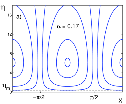
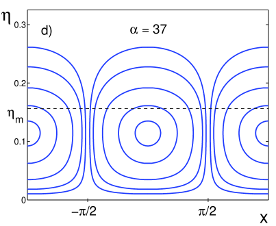
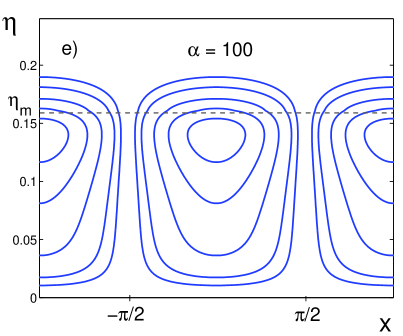
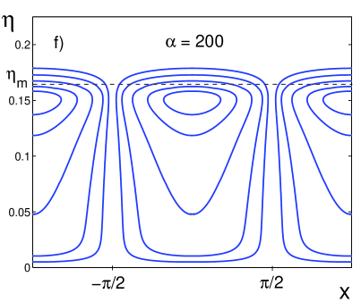
Figure 13: Stream–lines for $\Delta\Phi{\,=\,}100,\ \varepsilon{\,=\,}0.001$ and different values of $\alpha$.

C. Results for the linear stability analysis.

The final step of our analysis is to find $\hat{\Gamma}$ in the electro–neutral region, $\eta>\eta_{m}$, and solve the stability problem. Boundary conditions for $\Gamma$ at $\eta=\eta_{m}$ are

$$\hat{\Gamma}=\frac{G(r)}{\alpha}\hat{J},\ \ \ \frac{d\hat{\Gamma}}{d\eta}=-\left(3\alpha a\left(r\right)+2\eta_{m}\right)\frac{G(r)}{\alpha}\hat{J}\ \ \ \mbox{for}\ \ \ \eta=\eta_{m}.$$

Further it will be suitable to normalize $\hat{\Gamma}$ to $G\hat{J}/\alpha$,

$$\frac{d^{2}\hat{\Gamma}}{d\eta^{2}}+2\eta\frac{d\hat{\Gamma}}{d\eta}-\alpha^{2}\hat{\Gamma}=\frac{2\varkappa J}{\alpha\varepsilon^{2}}\>e^{\alpha\eta_{m}+\eta_{m}^{2}}\left(v+\alpha\left(u-v\right)(\eta_{m}-\eta)\right)e^{-\alpha\eta-\eta^{2}},$$ (106)

$$\ \ \displaystyle\hat{\Gamma}=1,\ \ \ \frac{d\hat{\Gamma}}{d\eta}=-3\alpha a-2\eta_{m}\ \ \ \mbox{for}\ \ \ \eta=\eta_{m}\\ ,$$ (107)

$$\hat{\Gamma}\to 0\ \ \ \mbox{at}\ \ \ \eta\to\infty.$$ (108)

The present asymptotic analysis in small $\varepsilon$ for the limiting regimes has no restrictions for the value of $\alpha$. The system (106)–(107) is solved numerically by the shooting method, and the calculated marginal stability curves are presented in Fig. 14. In this picture results of the numerical analysis without any restriction on $\alpha$ and $\varepsilon$ are presented [10]. The error of the present asymptotics can be significant near the nose of the marginal stability curves, but small far from it. This occurs since the nose of the marginal curve is located near the transition region from the under–limiting to limiting regime (see Fig. 3), where our asymptotics is not accurate.

Since the dimensionless Debye thickness and wave number are slow functions of time at moderately long times, we obtain, using for clearness the dimensional variables (denoted by tilde):

$$\varepsilon=\frac{\tilde{\lambda}_{D}}{\sqrt{4\tilde{D}\tilde{t}}},\ \ \ \ \alpha=\tilde{\alpha}\sqrt{4\tilde{D}\tilde{t}}.$$

Note that the coefficients of the eigenvalue problem (106)–(107) are slowly varied with time. Note also that in spite of their slow changing, the parametric dependence of $\alpha$ and $\varepsilon$ on time significantly changes the interpretation of the marginal stability curves. Taking this into account and following Shtemler (1981) [53], we present our neutral curves in coordinates $1/\varepsilon$ and $\alpha$, taking $\Delta\Phi$ as a constant parameter. The instantaneous values of $1/\varepsilon$ and $\alpha$ depend on time implicitly, $\alpha\sim\sqrt{4\tilde{D}\tilde{t}}$ and $1/\varepsilon\sim\sqrt{4\tilde{D}\tilde{t}}$ with the constant ratio

$$k=\frac{\alpha}{1/\varepsilon}=\frac{\tilde{\alpha}}{1/\tilde{\varepsilon}}=\tilde{\alpha}\tilde{\lambda}_{D}$$

Hence, any straight line which starts in the origin of the plane $(1/\varepsilon,\ \alpha)$ with inclination $k$

$$\alpha=k\frac{1}{\varepsilon}$$ (109)

characterizes wave number $\tilde{\alpha}$ constant with respect to time. If time is increasing, the instantaneous values of $1/\varepsilon$ and $\alpha$ lying on this line are increasing as $\sqrt{4\tilde{D}\tilde{t}}$. For large enough $k$, the whole straight line is in the stable region. Then, if we decrease the tangent $k$, at some $k=k_{0}$ the line (109) will be tangential to the neutral curve (see Fig. 15, upper left corner). The dependences of $k_{0}$, $\alpha_{0}=\alpha(k_{0})$ and $1/\varepsilon_{0}=1/\varepsilon(k_{0})$ as functions of $\Delta\Phi$ are given in Table 1.

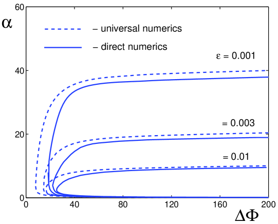
Figure 14: Marginal stability curves for self–similar asymptotic in $\varepsilon$ solution (106)–(107) (dashed lines) and exact numerical solution (solid lines) [10].

Figure 15: Marginal stability curves in $1/\varepsilon$ and $\alpha$ coordinates.

With further decrease of $k<k_{0}$, the straight line crosses the neutral curve in two points, $1$ and $1^{\prime}$, and the region along the line can be divided into three regions: I – the region between the origin and point $1$; II – the region within the neutral curve, between points $1$ and $1^{\prime}$; III – the region lying above the upper branch of the neutral curve.

$\Delta\Phi$	$k_{0}$	$\alpha_{0}$	$1/\varepsilon_{0}$	$Q(\Delta\Phi)$	$R(\Delta\Phi)$
$15$	$0.02$	$4.38$	$218.8$	$0.14$	$1.83$
$20$	$0.06$	$3.36$	$57.9$	$0.24$	$0.96$
$30$	$0.104$	$2.69$	$25.85$	$0.33$	$0.526$
$45$	$0.14$	$2.43$	$17.62$	$0.4$	$0.321$
$70$	$0.15$	$2.43$	$14.17$	$0.43$	$0.194$
$100$	$0.17$	$2.43$	$16.08$	$0.45$	$0.134$

Table 1: Critical parameters which separate stable and unstable regions (tangent $k_{0}$, wave number $\alpha_{0}$ and $1/\varepsilon_{0}$); and $Q$ and $R$ are functions of $\Delta\Phi$.

The initial point $(1/\varepsilon,\alpha)$ belonging to region I corresponds to decaying perturbations, but with increasing time the instantaneous values of $(1/\varepsilon,\alpha)$ intersect the lower branch of the neutral curve in point $1$ and enter the instability region. For $(1/\varepsilon,\alpha)$ in region II, the perturbations are increasing until the instantaneous values $(1/\varepsilon,\alpha)$ intersect the upper branch of the neutral curve; after this instant moment they begin to decay. For $(1/\varepsilon,\alpha)$ in region III, the perturbations decrease monotonically at all times.

It is possible to show that for $k<k_{0}$ the straight lines always leave the instability region. Indeed, from (52), (53) in combination with (57), (58) the asymptotics for the V–C curve as $\varepsilon\to 0$ can be obtained

$$\eta_{m}^{3}\sim\frac{9\sqrt{\pi}}{32}(\varepsilon\Delta\Phi)^{2}$$

just from this relation

$$r=\alpha\eta_{m}\sim\left(\frac{9\sqrt{\pi}\Delta\Phi^{2}}{32}\right)^{1/3}\alpha\varepsilon^{2/3}.$$ (110)

Now the upper branch of the marginal stability curves in short–wave approximation, $\alpha\to\infty$, can be readily obtained. In particular, we can claim that

$$\alpha\sim Q(\Delta\Phi)\left(\frac{1}{\varepsilon}\right)^{2/3},$$ (111)

where the function $Q(\Delta\Phi)$ is calculated numerically and presented in Table 1.

In order to evaluate the lower marginal stability branch, it is supposed that

$$\alpha\sim R(\Delta\Phi).$$ (112)

At $\varepsilon\to 0$ the relation becomes exact. The dependence $R(\Delta\Phi)$ is tabulated in Table 1.

The relations (111) and (112) allow, in particular, to estimate the time gap $\Delta\tilde{t}$ in which the perturbation with $k<k_{0}$ belongs to the instability region, between points $1$ and $1^{\prime}$, in Fig. 15,

$$\Delta\tilde{t}=\tilde{t}^{\prime}-\tilde{t}\sim\frac{k^{4}Q^{6}-R^{2}}{4\tilde{\alpha}^{2}\tilde{D}}.$$

This relation becomes exact at $k=\tilde{\alpha}\tilde{\lambda}_{D}\to 0$.

VI. CONCLUSIONS AND DISCUSSION

Electro–convective processes in an electrolyte solution between a semi–selective ion–exchange membranes have been investigated numerically and asymptotically in the limit of small Debye length $\varepsilon$. First, a simplified system of equations has been derived from the full system of equations that describes the ion transport and contains the Poisson and Stokes equations. Asymptotic expansions in small dimensionless Debye length are applied to both equilibrium and stability problems for the limiting regimes. Only the outer solution has been considered, ignoring the input of the surface and internal boundary layers. A novel class of the 1D unsteady self–similar solutions is found. A linear stability of these solutions and transition to electro–convection is considered. The marginal stability curves are constructed both numerically and asymptotically.

The results of stability modelling in small $\varepsilon$ are in fair agreement with those obtained by direct numerical simulations of the entire problem everywhere except for the vicinity of the critical point of the marginal stability curves. The possible reason of that deviation is that the critical point of the marginal curves is located near the transition region from the under–limiting to limiting regimes, while our asymptotics is valid only for the limiting regimes.

ACKNOWLEDGMENTS

E.A.D. is grateful to I.Rubinstein for his stimulating questions and remarks and to V. V. Nikonenko for numerous discussions and significant help in understanding the physical pattern the process.

Figure Captions

• Schematic V–C curve for ion–exchange membranes. A, B and C represent under–limiting, limiting and over–limiting regimes, respectively; * depicts the threshold of the over–limiting regimes; $C_{I}$ and $C_{II}$ are the regions of regular and irregular current oscillations; $j$ and $j_{lim}$ are the current density at the bottom membrane and its limiting value; $\Delta V$ is the potential drop.

• Schematic for limiting processes in a steady–state equilibrium: a) electric field $E{\,=\,}d\Phi/dy$; b) volume charge density $\rho{\,=\,c^{+}\,-\,}c^{-}$; c) ion concentrations $c{\,=\,}c^{+}$ and $c{\,=\,}c^{-}$. The dashed line is the outer solution in the small vicinities of $y{\,=\,}0$ (the double ion boundary layer) and $y{\,=\,}y_{m}$ (the boundary layer between the volume space charge region and the diffusion layer). The solid and dashed lines depict exact and asymptotic solutions for small $\varepsilon$.

• Marginal stability curves at different $\varepsilon$, numerics. The under–limiting regimes are stable (adopted from Demekhin et al. [10]).

• Self–similar charge $\rho=c^{+}-c^{-}$ (a) and concentration $c^{+}$ distribution (b) for different $\varepsilon$. Curves correspond to the following values of electric potential drop: 1. $\Delta\Phi=50$; 2. $\Delta\Phi=100$; 3. $\Delta\Phi=150$; 4. $\Delta\Phi=200$.

• VC curves. Comparison of the self–similar asymptotics (dashed lines) and the exact numerics (solid lines) for several $\varepsilon$.

• Distribution of the charge density $\rho$ in space for several moments of time, $\Delta V=100$ and $\nu{\,=\,}\tilde{\lambda}_{D}/\tilde{L}=0.001$. Solid line corresponds to the numerical solution of the unsteady problem (32)–(36). Two–parametric self–similar solution of (28)–(31) with $\varepsilon$ and $\Delta\Phi$ parametrically changing with time is depicted by dashed lines.

• Typical evolution of $1/j(t)$. I is the short–time region of influence of the initial data; II is the intermediately–long–time region of self–similarity, and III is the region of influence of the upper membrane $y{\,=\,}1$, ($\Delta V{\,=\,}100$ and $\nu{\,=\,}\tilde{\lambda}_{D}/\tilde{L}{\,=\,}0.001$).

• VC curves. Solid line relates to (54), while dashed line – to the simplified version (58).

• Negative ion concentration (a), $c^{-}$, and electric field (b), $H$, vs $y$ for several moments of time. Comparison of numerics (13)–(18) (solid lines) with self–similar asymptotics (49)–(50) (dashed lines) for (a) $\Delta V{\,=\,}50$, $\nu{\,=\,}0.001$: 1. $t{\,=\,}0.0001$; 2. $t{\,=\,}0.001$; 3. $t{\,=\,}0.004$; 4. $t{\,=\,}0.015$; 5. $t{\,=\,}0.5$; and (b) $\Delta V{\,=\,}100$, $\nu{\,=\,}0.0005$: 1. $t{\,=\,}0.001$; 2. $t{\,=\,}0.003$; 3. $t{\,=\,}0.03$.

• Comparison of the V–C characteristics for self–similar solution and numerics, $\Delta V=50,\nu=0.00005$. Numerics (13)–(18) is shown by squares and the universal self–similar VC curve (54) – by solid line. The region of the solution self–similarity $t_{1}{\,<\,t\,<\,}t_{2}$, $t_{1}\gg\nu^{2}/4$, $t_{2}\ll t_{s}=\tilde{L}^{2}/(4\tilde{D})$. Arrows depict the time growth along the voltage–current curve.

• Numerical points for several values of the potential drop between the membranes, $\Delta V$, shrink into the universal VC curve $J(\Delta F)$ given by (54); a) $\nu{\,=\,}0.001$, b) $\nu{\,=\,}0.0005$.

• Components of scaled slip velocities $u$ and $v$.

• Stream–lines for $\Delta\Phi{\,=\,}100,\ \varepsilon{\,=\,}0.001$ and different values of $\alpha$.

• Marginal stability curves for self–similar asymptotic in $\varepsilon$ solution (106)–(107) (dashed lines) and exact numerical solution (solid lines) [10].

• Marginal stability curves in $1/\varepsilon$ and $\alpha$ coordinates.

• The universal functions a) $G{\,=\,}G(r)$, b) $a{\,=\,}a(r)$.

Table Caption

• Critical parameters which separate stable and unstable regions (tangent $k_{0}$, wave number $\alpha_{0}$ and $1/\varepsilon_{0}$); and $Q$ and $R$ are functions of $\Delta\Phi$.

A. Electrostatic solution in the space charge region

Substituting a new independent variable $\displaystyle\xi=\alpha\left(\eta_{m}-\eta\right)$ into (91)–(92) results in:

$$\xi^{\frac{1}{2}}\frac{d^{2}}{d\xi^{2}}\left(\xi^{\frac{1}{2}}\frac{d\hat{F}}{d\xi}\right)-\xi\frac{d\hat{F}}{d\xi}-\hat{F}=0$$ (113)

$$\ \ \hat{F}=0\ \ \mbox{for}\ \ \ \xi=0$$ (114)

$$\ \ \hat{F}=0\ \ \mbox{for}\ \ \ \xi=r.$$ (115)

where $r=\alpha\eta_{m}$. The additional conditions which originate from (92) are:

$$\sqrt{\frac{2\alpha}{J}}\xi^{\frac{1}{2}}\frac{d\hat{F}}{d\xi}\to-\hat{\eta}_{m}\ \ \ \mbox{at}\ \ \ \xi\to 0,$$ (116)

$$\alpha\sqrt{\frac{J}{2\eta_{m}}}\left(2r\frac{d^{2}\hat{F}}{d\xi^{2}}+\frac{d\hat{F}}{d\xi}\right)=-\hat{J}\ \ \ \mbox{for}\ \ \ \xi=r.$$ (117)

We present the solution of (113)–(115) as

$$\hat{F}=B\sqrt{\xi}f(\xi)$$ (118)

where $B$ is constant. The equation (113) turns into

$$\xi f^{\prime\prime\prime}+\frac{5}{2}f^{\prime\prime}-\xi f^{\prime}-\frac{3}{2}f=0.$$

The general regular solution of this equation, up to a constant factor, has the form $\hat{F}=B\sqrt{\xi}\left(f_{1}\left(\xi\right)+af_{2}\left(\xi\right)\right)$, where $f_{1}$ and $f_{2}$ are two linearly independent solutions of the equation, $a$ is determined below. Solutions $f_{1}$, $f_{2}$, can be easily found numerically. Instead, for comparison convenience with long–wave asymptotics, the solution is presented as power expansions

$$f_{1}\left(\xi\right)=\sum_{n=0}^{\infty}{a_{2n}\xi^{2n}},\ \ \ \displaystyle f_{2}\left(\xi\right)=\sum_{n=0}^{\infty}{a_{2n+1}\xi^{2n+1}},$$ (119)

where $\displaystyle a_{k}\sim 1/k!$, and the series have infinite radius of convergence

$$\begin{array}[]{c}a_{2n}=\displaystyle\frac{1}{(2n)!}\prod_{k=1}^{n}\frac{4k-1}{4k+1},\ \ \ a_{0}=1,\\[12.0pt] a_{2n+1}=\displaystyle\frac{1}{(2n+1)!}\prod_{k=1}^{n}\frac{4k+1}{4k+3},\ \ \ \ a_{1}=1.\end{array}$$ (120)

Note that the long wave limit is described by a finite term expansion (119).

Assuming

$$f=f_{1}+af_{2}=0$$

at some $\alpha\eta_{m}=r\left(a\right)$, the second BC (115) for $\hat{F}$ is satisfied. Let us invert the function $r=r(a)$,

$$a(r)=-\frac{f_{1}(r)}{f_{2}(r)},\ \ \ r=\alpha\eta_{m}.$$ (121)

Thus we obtain, taking into account (118), that the function $\hat{F}$ satisfies the first two boundary conditions (114)–(115). The constant $B$ is obtained by substitution of (118) into (117),

$$\hat{\eta}_{m}=-\frac{G\left(r\right)}{\alpha}\frac{\hat{J}}{J},\ \ \ G(r)=-\frac{1}{2rf^{\prime\prime}(r)+3f^{\prime}(r)}.$$ (122)

where $f^{\prime},\ f^{\prime\prime}$ are taken at $\xi=r$ and are functions of $r$, $G=G\left(r\right)$ is the universal function shown along with $a(r)$ in Fig. 16.

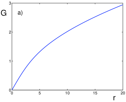
Figure 16: The universal functions a) $G{\,=\,}G(r)$, b) $a{\,=\,}a(r)$.

Then we get the unknown function $\hat{F}$,

$$\hat{F}=-\sqrt{\frac{2J}{\alpha}}\>\hat{\eta}_{m}\sqrt{\xi}f(\xi),\ \ \ \xi=\alpha\left(\eta_{m}-\eta\right).$$ (123)

Substituting (123) into (93), we obtain the relation for the outer expansion of the charge density $\hat{\rho}$,

$$\hat{\rho}=\varepsilon\sqrt{2J\alpha^{3}}\>\hat{\eta}_{m}\left[\sqrt{\xi}f\>^{\prime\prime}+\frac{1}{\xi}f\>^{\prime}-\left(\frac{1}{4\xi\sqrt{\xi}}+\sqrt{\xi}\right)f\right].$$ (124)

which has a singularity at $\eta=\eta_{m}$.

Furthermore, from (119)–(121), the asymptotic expansions for $a(r)$ and $G(r)$ as $r\rightarrow 0$ can be found

$$a(r)=-\frac{\sum_{n=0}^{\infty}{a_{2n}r^{2n}}}{\sum_{n=0}^{\infty}{a_{2n+1}r^{2n+1}}}.$$ (125)

For small $r$, which corresponds to the long–wave approximation ($\alpha\rightarrow 0$),we obtain,

$$a\left(r\right)=-\frac{1}{r}-\frac{19}{105}r+\frac{169}{24255}r^{3}+\cdots\sim-\frac{1}{r},\ \ r\rightarrow 0.$$ (126)

From (122), in the first approximation with respect to $r$,

$$G\left(r\right)=\frac{1}{3}\,r-\frac{1}{210}\,r^{3}+\frac{59}{415800}\,r^{5}+\cdots\sim\frac{1}{3}\,r,\ \ r\rightarrow 0.$$ (127)

and

$$\hat{\eta}_{m}=\eta_{m}\frac{{\hat{J}}}{J}\left(-\frac{1}{3}+\frac{1}{210}(\alpha\eta_{m})^{2}-\frac{59}{415800}(\alpha\eta_{m})^{4}+\cdots\right)\sim-\frac{\eta_{m}}{3}\frac{{\hat{J}}}{J}.$$ (128)

Approximation (127)–(128) is valid at $r<1.5\div 2$.

The asymptotics of $f_{1}$ and $f_{2}$ at $\xi\rightarrow\infty$ are useful in the short–wave approximation $\alpha\to\infty$ of the stability problem. They can be readily found by asymptotic expansions of the equation (113):

$$f_{1}\sim\frac{const_{1}}{\sqrt{\xi}}\>e^{\xi},\ \ \ \ f_{2}\sim\frac{const_{2}}{\sqrt{\xi}}\>e^{\xi},\ \ \ \ \xi\rightarrow\infty.$$

At $r\rightarrow\infty$

$$a(r)\sim a_{*},\ \ \ G\left(r\right)\sim c_{*}\sqrt{r},$$ (129)

where

$$a_{*}\approx-0.72948,\qquad c_{*}\approx 0.66468.$$

B. Components of the slip velocity

Now the obtained function $\hat{F}$ can be used to solve the hydrodynamic problem (94), (95), (96) and find the stream function perturbation $\hat{\Psi}$. The slip velocity components $\hat{\Psi}\left(\eta_{m}\right)=i\hat{V}_{m}$ and $\hat{\Psi}\>\left(\eta_{m}\right)=\hat{U}_{m}$ specify the boundary conditions for the problem in the electro–neutral region $\eta_{m}<\eta<\infty$.

Taking the variable $\xi=\alpha(\eta_{m}-\eta)$ with $r=\alpha\eta_{m}$, and utilizing relations (122), (123), the problem (94)–(96) can be reformulated as

$$\frac{d^{4}\psi}{d\xi^{4}}-2\frac{d^{2}\psi}{d\xi^{2}}+\psi=\xi\left(\frac{d^{2}f}{d\xi^{2}}-f\right)+\frac{df}{d\xi},$$ (130)

$$\begin{array}[]{c}\displaystyle\frac{d^{2}\psi}{d\xi^{2}}-2\frac{d\psi}{d\xi}+\psi=0,\ \ \ \frac{d^{3}\psi}{d\xi^{3}}-3\frac{d\psi}{d\xi}+2\psi=0\ \ \ \mbox{for}\ \ \ \xi=0,\\ \displaystyle\psi=\frac{d\psi}{d\xi}=0\ \ \ \mbox{for}\ \ \ \xi=r,\end{array}$$ (131)

where

$$\psi\left(\xi,r\right)=\frac{1}{i\hat{C}}\hat{\Psi},\ \ \ C=\frac{2\varkappa}{\varepsilon^{2}\alpha^{4}}\>G\left(r\right)\hat{J}.$$ (132)

$\hat{V}_{m}$ and $\hat{U}_{m}$ are used as the boundary condition for the hydrodynamic problem in the electro–neutral region $\eta>\eta_{m}$,

$$\hat{V}_{m}=\hat{C}v\left(r\right)\equiv\hat{C}\psi\left(0,r\right),\ \ \ \hat{U}_{m}=-i\alpha\hat{C}u\left(r\right)\equiv-i\alpha\hat{C}\frac{\partial\psi}{\partial\xi}\left(0,r\right).$$ (133)

The function $f$ in the right hand side of (130) is

$$\xi\left(\frac{d^{2}f}{d\xi^{2}}-f\right)+\frac{df}{d\xi}\stackrel{{\scriptstyle def}}{{=}}g=g_{1}+ag_{2},$$

where

$$\begin{array}[]{c}\displaystyle g_{1}=\sum_{n=0}^{\infty}b_{2n+1}\xi^{2n+1},\ \ \ \ b_{2n+1}=\frac{a_{2n}}{\left(2n+1\right)\left(4n+5\right)},\\ \displaystyle\displaystyle g_{2}=\sum_{n=0}^{\infty}b_{2n}\xi^{2n},\ \ \ \ b_{2n}=\frac{a_{2n-1}}{2n\left(4n+3\right)},\ \ b_{0}=1.\end{array}$$ (134)

Then the solution of (130)–(131) can be presented in the form

$$\psi=(A+B\xi)e^{\xi}+\psi_{p}\>,\ \ \ \psi_{p}=\psi_{1}+a\psi_{2}\>,$$ (135)

where $e^{\xi}$ and $\xi e^{\xi}$ – are two linearly independent solutions which satisfy the first two conditions (131) at $\xi{\,=\,}0$, $A$, $B$ – some constants, $\psi_{p}$ is a particular solution of (130) which satisfies zero conditions

$$\psi_{p}=\frac{d\psi_{p}}{d\xi}=\frac{d^{2}\psi_{p}}{d\xi^{2}}=\frac{d^{3}\psi_{p}}{d\xi^{3}}=0,\ \ \ \xi=0.$$ (136)

Functions $\psi_{1}$ and $\psi_{2}$ – are the odd and even components of $\psi_{p}$, which can be found from solutiion (130) with right–hand side $g_{1}$ and $g_{2}$ correspondingly and boundary conditions (136). They can be presented as expansions

$$\begin{array}[]{ll}\displaystyle\psi_{1}=\sum_{n=2}^{\infty}c_{2n+1}\xi^{2n+1},&\displaystyle\ \ \ c_{2n+1}=\sum_{k=0}^{n-2}\frac{\left(n-k-1\right)\left(2k+1\right)!}{\left(2n+1\right)!}\,b_{2k+1},\\[12.0pt] \displaystyle\psi_{2}=\sum_{n=2}^{\infty}c_{2n}\xi^{2n},&\displaystyle\ \ \ c_{2n}=\sum_{k=0}^{n-2}\frac{\left(n-k-1\right)\left(2k\right)!}{\left(2n\right)!}\,b_{2k}\end{array}$$ (137)

The constants $A,B$ are found from the BC’s at $\xi=r$,

$$A=\left(r\frac{d\psi_{p}(r)}{d\xi}-(1+r)\psi_{p}(r)\right)e^{-r},\ \ \ \ B=\left(\psi_{p}(r)-\frac{d\psi_{p}(r)}{d\xi}\right)e^{-r}.$$ (138)

Taking into account (133) yields

$$v=A=\left(r\frac{d\psi_{p}(r)}{d\xi}-(1+r)\psi_{p}(r)\right)e^{-r},$$ (139)

$$u=A+B=\left((r-1)\frac{d\psi_{p}(r)}{d\xi}-r\psi_{p}(r)\right)e^{-r},$$ (140)

The obtained relations provide a complete description for the slip velocity components $\hat{U}_{m}$ and $\hat{V}_{m}$ according to (133).

Finally, let us present the Taylor series near $r=0$ for the slip velocity in the long–wave approximation. Using (126), (135) and (137), we can write the following relation,

$$\psi_{p}\left(r\right)=\sum_{k=1}^{\infty}c_{2k+3}r^{2k+3}-\frac{\sum_{k=0}^{\infty}a_{2k}r^{2k}}{\sum_{k=0}^{\infty}a_{2k+1}r^{2k+1}}\sum_{k=1}^{\infty}c_{2k+2}r^{2k+2},$$ (141)

where the series coefficients are calculated according to (120) and (134), (135). Expanding the exponents in (139), (140) in series in the vicinity of $r=0$, re–expanding them and differentiating the above relation with respect to $r$, the functions $u(r)$ and $v(r)$ are obtained,

$$\begin{array}[]{l}\displaystyle v(r)=-\frac{1}{8}r^{3}+\frac{1}{6}r^{4}-\frac{27}{200}r^{5}+\cdots,\\[7.0pt] \displaystyle u(r)=\frac{1}{6}r^{2}-\frac{1}{3}r^{3}+\frac{167}{504}r^{4}+\cdots.\end{array}$$ (142)

All the series in (141) converge at any $r$, while the series (142) have finite convergence radius because of above mentioned hidden singularity of the universal function $a=a(r)$ in the complex plane.

We find the limiting values of $u$ and $v$,

$$v\rightarrow v_{\infty}\approx-0.27245,\ \ \ \ u\rightarrow u_{\infty}\approx-0.12437\ \ \ \ \mbox{as}\ \ r\rightarrow\infty.$$ (143)

Moreover, $u$ changes sign at $r=\alpha\eta_{m}\approx 1.59523$. The dependence of $u$ and $v$ on $r$ is shown in Fig. 12. At $r\to 0$ results can be obtained in a closed form; they coincide with obtained in [47].

References

- [1] W. H. Smyrl and J. Newman, “Double layer structure at the limiting current,” Trans. Faraday Soc. 63, 207 (1967).
- [2] R. P. Buck, “Steady state space charge effects in symmetric cells with concentration polarized electrodes,” J. Electroanal. Chem. Interf. Electrochem. 46, 1 (1973).
- [3] I. Rubinstein and L. Shtilman, “Voltage against current curves of cation exchange membranes,” J. Chem. Soc. Faraday Trans. II 75, 231 (1979).
- [4] V. V. Nikonenko, V. I. Zabolotsky and N. P. Gnusin, “Electric transport of ions through diffusion layers with impaired electroneutrality,” Sov. Elektrochem. 25, 301 (1989).
- [5] A. V. Listovnichy, “Passage of currents higher than the limiting one through the electrode–electolyte solution system”, Sov. Electrochem. 51, 1651 (1989).
- [6] J. A. Manzanares, W. D. Murphy, S. Mafe and H. Reiss, “Numerical simulation of the nonequilibrium diffuse double layer in ion–exchange membranes”, J. Phys. Chem. 97, 8524 (1993).
- [7] V. A. Babeshko, V. I. Zabolotsky, N. M. Korzhenko, R. R. Seidov, and M. A.–Kh. Urtenov, “The theory of steady–state transport of binary electrolyte in a one–dimensional case”, [in Russian] Dokl. Akad. Nauk 361, 41 (1998).
- [8] K. T. Chu and M. Z. Bazant, “Electrochemical thin films at and above the classical limiting current,” SIAM J. Appl. Math. 65, 1485 (2005).
- [9] B. Zaltzman and I. Rubinstein, “Electroosmotic slip and electroconvective instability”, J. Fluid Mech. 579, 173 (2007).
- [10] E. A. Demekhin, E. M. Shapar, and V.V. Lapchenko, “Initiation of electroconvection in semipermeable electric membranes”, Doklady Physics 53, 450 (2008).
- [11] G. Yossifon and H.–C. Chang, “Selection of nonequilibrium overlimiting currents: universal depletion layer formation dynamics and vortex instability”, Phys. Rev. Lett. 101, 254501 (2008).
- [12] L. G. Levich. Physicochemical Hydodynamics, Prentice–Hall, New York, 1962.
- [13] B. M. Grafov and A. A. Chernenko, “Theory of passage of a constant current through a solution of a binary electrolyte”, [in Russian] Dokl. Akad. Nauk SSSR, 146, 135 (1962).
- [14] M. A.–Kh. Urtenov, E. V. Kirillova, N. M. Seidova, and V.V. Nikonenko, “Decoupling of the Nernst–Plank and Poisson equations. Applications to a membrane system at overlimiting currents”, J. Phys. Chem. B 111, 14208 (2007).
- [15] V. A. Babeshko, V. I. Zabolotsky, E. V. Kirillova, and M. A.–Kh. Urtenov, “Decomposition of Nernst–Planck–Poisson equations,” [in Russian] Dokl. Akad. Nauk 344, 485 (1995).
- [16] V. A. Babeshko, V. I. Zabolotsky, N. M. Korzhenko, R. R. Seidov, and M. A.–Kh. Urtenov, “Theory of stationary transport of a binary electrolite in one–dimensional case”, [in Russian] Rus. J. Electrochem. 8, 863 (1997).
- [17] V. A. Babeshko, V. I. Zabolotsky, N. M. Korzhenko, R. R. Seidov, and M. A.–Kh. Urtenov, “Theory of stationary transport of a binary electrolite in one–dimensional case. Numerical analysis,” [in Russian] Dokl. Akad. Nauk 355, 488 (1997).
- [18] V. A. Babeshko, V. I. Zabolotsky, R. R. Seidov, and M. A.–Kh. Urtenov, “ Decomposition equations for the stationary transport of electrolite in one–dimensional case”, [in Russian], Rus. J. Electrochem. 33, 855 (1997).
- [19] M. A.–Kh. Urtenov and R. R. Seidov. Mathematical models for the electrical membranes for water purification, [in Russian] KubSU, Krasnodar, 2000.
- [20] M. A.–Kh. Urtenov, “Mathematical models for the electrical membranes for water purification”, [in Russian] Doctor Thesis, KubSU, Krasnodar, 2001.
- [21] M. A.–Kh. Urtenov. Boundary problems for the electrical membranes for water purification, [in Russian] KubSU, Krasnodar, 1998.
- [22] S. V. Polyanskikh, ‘Electrohydrodynamic stability of some microflows with concentration polarization‘”, [in Russian] Ph. D. Thesis, Moscow State University, Moscow, 2010.
- [23] M. Van Dyke. Perturbation Methods in Fluid Mechanics, Academic Press, New York, 1964.
- [24] E.I. Belova, G.Yu. Lopatkova, N.D. Pismenskaya, V. V. Nikonenko, C. Larchet, and G. Pourcelly, “Effect of anion–exchange membrane surface properties on mechanisms of overlimiting mass transfer”, J. Phys. Chem. B 110, 13458 (2006).
- [25] N.D. Pismenskaya, V. V. Nikonenko, E. I. Belova, G. Yu. Lopatkova, Ph. Sistat, G. Pourcelly, and K. Larshe, “Coupled convection of solution near the surface of ion–exchange membranes in intensive current regimes”, Rus. J. Electrochem. 43, 307 (2007).
- [26] M.C. Cross and P. G. Hohenberg, “Pattern fomation outside of equilibrium”, Rev. Modern Physics 65, 3, 851 (1993).
- [27] I. Rubinstein, E. Staude, and O. Kedem, “Role of the membrane surface in concentration polarization at ion–exchange membrane”, Desalination 69, 101 (1988).
- [28] F. Maletzki, H.W. Rossler, and E. Staude, “Ion transfer across electrodialysis membranes in the overlimiting current range: stationary voltage–current characteristics and current nouse power spectra under different condition of free convection”, J. Membr. Sci. 71, 105 (1992).
- [29] I. Rubinstein, B. Zaltzman, J. Pretz, and C. Linder, “Experimental verification of the electroosmotic mechanism of overlimiting conductance through a cation exchange electrodialysis membrane”, Rus. J. Electrochem. 38, 853 (2004).
- [30] S. M. Rubinstein, G. Manukyan, A. Staicu, I. Rubinsten, B. Zaltzman, R. G. H. Lammertink, F. Mugele and M. Wessling, “Direct observation of nonequilibrium electroosmotic instability”, Phys. Rev. Lett. 101, 236101 (2008).
- [31] S. J. Kim, Y.–C. Wang, J. H. Lee, H. Jang and J. Han, “Concentration polarization and nonlinear electrokinetic flow near a nanofluidic channel”, Phys. Rev. Lett. 99, 044501.1 (2007).
- [32] A. P. Grigin, “The convective coulombic instability of binary electrolytes in cells with plane–parallel electrodes”, Sov. Electrochem. 21, 48 (1985).
- [33] A. P. Grigin, “Coulomb convection in electrochemical systems”, Sov. Electrochem. 28, 247 (1992).
- [34] I. Rubinstein, T. Zaltzman, and B. Zaltzman, “Electroconvection in a layer and in a loop”, Phys. Fluids 7, 1467 (1995).
- [35] R. Bruinsma and S. Alexander, “Theory of electrohydrodynamic instabilities in electrolytic cells”, J. Chem. Phys. 92, 3074 (1990).
- [36] R. S. Alexandrov, A. P. Grigin, and A. P. Davydov, “Numerical study of electroconvective instability of binary electrolyte in a cell with plane parallel electrodes”, Russian J. Electrochem. 38, 1097 (2004).
- [37] J. C. Baygents and F. Baldessari, “Electrohydrodynamic instability in a thin fluid layer with an electrical conductivity gradient”, Phys. Fluids 10, 301 (1998).
- [38] M. E. Buchanan and D. A. Saville, “Electrohydrodynamic stability in electrochemical systems”, in Proceedings of APS 53rd Annual Meeting, Nov. 19–21, Washington, DC (2000).
- [39] I. Lerman, I. Rubinstein and B. Zaltzman, “Absence of bulk electroconvective instability in concentration polarization”, Phys. Rev. E., 71, 011506 (2005).
- [40] S. S. Dukhin, “Electrokinetic phenomena of the second kind and their applications”, Adv. Coll. Interf. Sci. 35, 173 (1991).
- [41] S. S. Dukhin and N. A. Mishchuk, “Disappearance of limiting current phenomenon in the case of a granule of an ion–exchanger”, [in Russian] Kolloidn. Zh., 51, 570 (1990).
- [42] S. S. Dukhin, N. A. Mishchuk, and P. B. Takhistov, “Electroosmosis of the second kind and unrestricted current increase in the mixed monolayer of an ion–exchanger”, [in Russian] Kolloidn. Zh., 51, 540 (1989).
- [43] S. S. Dukhin and B. V. Derjaguin. Electrophoresis, 2nd edn. [in Russian] Nauka, Moscow, 1976.
- [44] E. K. Zholkovskii, M. A. Vorotynsev and E. Staude, “Electrokinetic instability of solution in a plane–parallel electrochemical cell”, J. Membrane. Sci. 181, 28 (1996).
- [45] M. Z. Bazant and T. M. Squires, “Induced–charge electro–kinetic phenomena: Theory and microfluidic applications”, Phys. Rev. Lett. 92, 066101 (2004).
- [46] I. Rubinstein and B. Zaltzman, “Electro–osmotically induced convection at a permselective membrane, ” Phys. Rev. E 62, 2238 (2000).
- [47] I. Rubinstein and B. Zaltzman, “Electro–osmotic slip of the second kind and instability in concentration polarization at electrodialysis membranes, ” Math. Mod. Meth.Appl. Sci., 11, 263 (2001).
- [48] I. Rubinstein and B. Zaltzman, “Wave number selection in a nonequilibrium electroosmotic instability”, Phys. Rev. E 68, 032501 (2003).
- [49] I. Rubinstein, B. Zaltzman, and I. Lerman, “Electroconvective instability in concentration polarization and nonequilibrium electro–osmotic slip”, Phys. Rev. 72, 011505 (2005).
- [50] T. Pundik, I. Rubinstein and B. Zaltzman, “Bulk electroconvection in electrolyte”, Phys. Rev. E., 72, 061502 (2005).
- [51] V. I. Zabolotsky and V. V. Nikonenko. Ion transport in membranes, [in Russian] Nauka, Moscow, 1996.
- [52] L. I. Sedov. Similarity and dimensional metods in mechanics, 4–th edn. Academic Press, New York, 1977.
- [53] Yu. M. Shtemler, “Stability of unsteady viscous flows”, [in Russian] Izv. A. N. USSR. Mech. Zhidk. i Gaza. 4, 138 (1981).
- [54] C. C. Lin. The theory of hydrodynamic instability, Cambridge University Press, Cambrige, 1967.