The Importance of XUV Radiation as a Solution to the P v Mass Loss Rate Discrepancy in O-Stars

Abstract

A controversy has developed regarding the stellar wind mass loss rates in O-stars. The current consensus is that these winds may be clumped which implies that all previously derived mass loss rates using density-squared diagnostics are overestimated by a factor of $\approx$ 2. However, arguments based on FUSE observations of the P v resonance line doublet suggest that these rates should be smaller by another order of magnitude, provided that P v is the dominant phosphorous ion among these stars. Although a large mass loss rate reduction would have a range of undesirable consequences, it does provide a straightforward explanation of the unexpected symmetric and un-shifted X-ray emission line profiles observed in high energy resolution spectra. But acceptance of such a large reduction then leads to a contradiction with an important observed X-ray property: the correlation between He-like ion source radii and their equivalent X-ray continuum optical depth unity radii. Here we examine the phosphorous ionization balance since the P v fractional abundance, $q$ (P v), is fundamental to understanding the magnitude of this mass loss reduction. We find that strong “XUV” emission lines in the He ii Lyman continuum can significantly reduce $q$ (P v). Furthermore, owing to the unique energy distribution of these XUV lines, there is a negligible impact on the S v fractional abundance (a key component in the FUSE mass loss argument). We conclude that large reductions in O-star mass loss rates are not required, and the X-ray optical depth unity relation remains valid.

1 Introduction

Over the past several years, questions concerning the validity of what we refer to as the “traditional” O-star mass loss rates, $\dot{M}$, have arisen owing to the predictions of clumped wind models (see recent Potsdam Workshop, Hamann et al. 2008, and references therein). Abbott et al. (1981) showed that inhomogeneous winds lead to an enhancement in density- squared emission processes such as H$\alpha$, infrared and radio free-free, which means that the inferred $\dot{M}$ would be overestimated (see also Puls et al. 2006). Although a clear picture of these clumpy structures is still being developed, the so-called “clumping factor” ($f_{cl}$) is believed to be $\approx$ 4 to 5, and the reduction in $\dot{M}$ scales with $\sqrt{f}_{cl}$ (see General Discussion in Hamann et al. 2008).

The derived $\dot{M}$ from diagnostics that are linearly dependent on density (e.g., analyses of unsaturated UV resonance line profiles) are expected to be independent of clumping effects (Puls et al. 2006) and supposedly should provide more reliable $\dot{M}$ values. In fact, analyses of the P v resonance line doublet ($\lambda\lambda$ 1118, 1128 Å) obtained from FUSE observations led to the conclusion that traditional $\dot{M}$ are overestimated by a factor of 10 or more (Massa et al. 2003, hereafter M03; Fullerton et al. 2006; hereafter F06). Such reductions have far-reaching consequences. For example, Hirschi (2008) concluded that the well known evolutionary tracks of massive stars could survive $\dot{M}$ reductions by a factor of 2, but not by a factor of 10 or more.

Resolution of this $\dot{M}$ problem is also of particular importance with regards to the observed X-ray emission line properties obtained from $Chandra$ and $XMM-Newton$ observations. Waldron & Cassinelli (2007) analyzed the Chandra HETGS X-ray line properties for a large number of OB stars, and two of their conclusions are directly relevant to this $\dot{M}$ issue. 1) All of the resolved X-ray emission lines are very broad (i.e., HWHM range of 300 to 1000 $km~{}s^{-1}$), symmetric, and the majority have minimal line-shifts. Although Waldron & Cassinelli (2001) were the first to demonstrate that these X-ray line profiles could in fact be easily explained by a significant reduction in $\dot{M}$, this was inconsistent with the then accepted observed $\dot{M}$, and they suggested a clumpy or non-symmetric wind structure as a possible explanation. 2) The radial locations of the He-like $fir$ (forbidden, intercombination, resonance) line sources, as derived from their $f/i$ line ratios, typically range from 1.2 to 10 $R_{*}$, and these distances are well correlated with their respective stellar wind X-ray continuum optical depth unity radii which we shall refer to as the “X-ray continuum optical depth unity relation” (hereafter abbreviated as XODUR). This relation implies that the traditional $\dot{M}$ (like those of Vink et al. 2000) must be correct (i.e., within a factor of 2 or so). Nevertheless, large $\dot{M}$ reductions have become a widely used explanation of the X-ray line profile symmetry problem (e.g., Kramer et al. 2003; Cohen et al. 2006) because the emission from both the near and far side of a star would be observable in an optically thin wind. The subject is not yet resolved since Oskinova et al. (2004, 2006) finds that the symmetry can also be explained by accounting for the porosity of clumped (or fragmented) winds without the need for a reduction in $\dot{M}$, but Owocki & Cohen (2006) present arguments against the porosity influence.

The primary goal of this paper is to examine the effects of an excess of hard radiation within the He ii Lyman continuum on the ionization equilibrium of phosphorus by utilizing only outer shell photoionization processes. This is important since the proposed large reduction in $\dot{M}$ is based entirely on the assumed P v fractional ionization abundance. In addition, we also consider the sulfur ionization balance because of two arguments used by M03 and F06: 1) since phosphorous and sulfur have overlapping ranges in ionization energy, the dominant stages of sulfur can be used as surrogates for the corresponding ones of phosphorous, and; 2) both P v and S v are likely to be the dominant ionization stages throughout the O-star spectral range.

We propose that the primary source of this excess hard radiation is produced by the “XUV” spectral energy band which has long been known to have the capability to produce anomalously higher wind ionization stages (e.g., Waldron 1984; MacFarlane et al. 1994; Pauldrach et al. 1994, 2001). Based on solar physics studies, the XUV lower energy bound seems to be rather loosely defined, but the upper limit appears to be fixed at 124 eV (100 Å) where the XUV upper limit represents the start of the X-ray energy band. For our purposes, we adopt an XUV radiation energy band defined as 54.4 eV (He ii edge) to 124 eV, since below the He ii edge, the radiation is dominated by photospheric emission. Although XUV radiation is un-detectable in O-stars, its effects can be manifested by studying other spectral bands. In particular, with regards to the two key arguments used by M03 and F06, we show that XUV radiation produces dissimilar changes in the phosphorous and sulfur ionization equilibria.

2 Importance of XUV Radiation

In this section we use graphical arguments to illustrate the importance of XUV radiation with respect to the total radiation cooling curve and the ionization equilibria of phosphorous and sulfur. To emphasize the importance of XUV + X-ray radiation, we provide comparisons with the case when only X-ray radiation is considered. Although unobservable, we believe an observational signature of XUV radiation has already been detected by M03. In their FUSE study of LMC stars, they explicitly state that “…C v is the dominant species for O stars”. This can only mean that there must be excess XUV emission since the C iv photoionization edge lies within the XUV energy range (see Fig. 2).

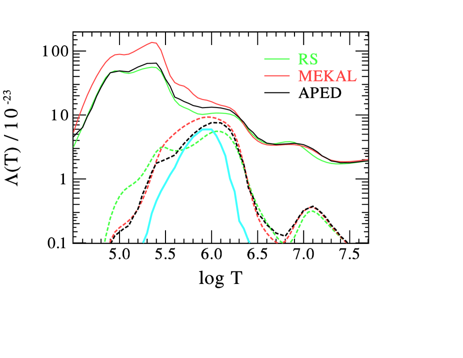
Figure 1: Comparison of radiative cooling curves determined from the RS, MEKAL, and APED emissivites. The dashed-line curves represent the contribution of the XUV radiation (54.4 - 124 eV) to the total cooling curve. The solid blue line represents the contribution from the important collection of XUV emission lines between 65 and 73 eV (See §2 and Fig. 2).

We first discuss the expected contribution of XUV radiation to the radiative cooling curve (e.g., Cox & Tucker 1969), $\Lambda(T)=P(T)/(n_{e}~{}n_{H}$) ( erg cm³ s^-1) where $P(T)$ is the power per unit volume and $n_{e}$ and $n_{H}$ are the electron and hydrogen number densities respectively. Although cooling curves have undergone alterations over the years (e.g., atomic data updates and added emission lines), the basic shape of the cooling curve has remained intact as shown in Figure 1. This shows $\Lambda(T)$ obtained from Raymond & Smith (1977; RS), Mewe et al. (1985; MEKAL), and Smith et al. (2001; APED) data. It also shows that the XUV contribution to $\Lambda(T)$ is clearly important for temperatures between 0.5 and 2.0 MK.

Since the photoionization edge for P v $\rightarrow$ P vi is at 65.03 eV, and that for S v $\rightarrow$ S vi is nearby at 72.68 eV, it seems plausible that their ionization balances should be quite similar. This similarity led to the F06 argument that S v can be used as a surrogate for P v. However, as shown in Figure 2, just beyond the P v photoionization edge there exists a large collection of intense XUV emission lines (their specific contribution is shown in Fig. 1) that are located just below the S v ionization energy. Whereas, at energies higher than this edge, the XUV emission at this temperature is essentially devoid of emission lines, i.e., all lines between the S v edge and 124 eV are at least a factor of 100 times smaller than the strongest line just below the S v edge. Consequently, this unique energy distribution of XUV lines relative to the energy locations of these photoionization edges indicates that the XUV emission should produce different effects on the phosphorous and sulfur ionization equilibria. This is illustrated in Figure 3 which shows that the P v photoionization rate is $\approx$ 10 times larger than the S v rate at the temperature of maximum XUV emission (see Fig. 1). Figure 3 includes the C iv rate for comparison, and also shows the expected photoionization rates using only the X-ray energy band ($\geq$ 124 eV). As evident from the displacement of these curves, the neglect of XUV radiation leads to underestimates of these rates which are substantial at temperatures $<$ 2 MK. This implies that alone, the radiation from the X-ray energy band is not expected to have a significant impact on the ionization equilibrium of phosphorous, as was recently demonstrated by Krticka & Kubat (2009) in their study of the Auger effect on the fractional abundance of P v.

Our graphical arguments illustrate that the XUV line emission for temperatures between 0.5 to 2 MK is expected to have a major impact on the ionization structure of phosphorous but a relatively minor effect on sulfur. This implies that the sulfur surrogate argument needs to be re-examined (see §3). In fact, since the C iv photoionization edge is almost identical to the P v edge (see Fig. 2), C iv is a more appropriate surrogate for P v. The main difference is that the C iv photoionization rate is larger than the P v rate (see Fig. 3) due to the differences in their cross sections.

3 Ionization Equilibrium Calculations and Required XUV Radiation

The stellar wind ionization equilibria of phosphorous and sulfur are calculated in a straightforward way to determine the level of XUV+X-ray radiation required to affect the fractional ionization abundances, i.e., $q$ (P v) and $q$ (S v). We consider a stellar effective temperature ($T_{eff}$) range from 27500 to 45000 K which covers the O and early B spectral range where P v has been used to study $\dot{M}$. The ionization equilibrium is determined by adopting an ionization/recombination rate balance approach similar to the one used in FASTWIND (Puls et al. 2005). The main differences are: 1) we use the photoionization cross sections of Verner & Yakovlev (1995); 2) a wind diffuse field as prescribed by Drew (1989), and; 3) we assume a radial power law dependent wind temperature ($T_{W}$) which is adjusted to produce a phosphorous wind ionization structure similar to that of Puls et al. (2008) (i.e., no XUV+X-ray radiation) for all $T_{eff}$ considered. This adjustment leads to a $T_{W}/\hbox{$T_{eff}$}=1.15(\hbox{$R_{*}$}/r)^{0.5}$ with a minimum value of $0.6\hbox{$T_{eff}$}$. We calculate $q$ (P v) and $q$ (S v) for wind conditions at a location where the wind velocity is $1/2$ the terminal velocity, $v_{\infty}$. For each $T_{eff}$, a consistent set of stellar parameters (log $g$, $L_{Bol}$, $R_{*}$) is found by using the fitting-formulae given by Martins et al. (2005). We use the electron scattering Eddington factor as described by Lamers (1981) to determine the effective escape velocity, $V_{esc}$. For the wind parameters, we use $\hbox{$v_{\infty}$}=2.6~{}\hbox{$V_{esc}$}$ and $\dot{M}$ predicted by the Vink et al. (2000) formula. The radially dependent wind density is determined from the mass conservation equation using a $\beta$-velocity law $V(r)=\hbox{$v_{\infty}$}(1-R_{*}/r)^{\beta}$ assuming a $\beta=0.8$ (Pauldrach et al. 1986; Müller & Vink 2008). The wind electron density is derived assuming hydrogen and helium are fully ionized.

The energy dependent mean intensity (erg cm^-2 s^-1 eV^-1 str^-1) used to calculate the photoionization rates has two dominant contributions: 1) the photospheric radiation field for a given $T_{eff}$ and appropriate log $g$ (using the TLUSTY grid of models from OSTAR2002, Lanz & Hubeny 2003), along with the standard geometric dilution factor, and; 2) the XUV+X-ray radiation field, $J_{\rm X}$. This $J_{\rm X}$ is specified by two parameters, the hot plasma temperature, $T_{\rm X}$, and the column emission measure, $\Delta EM_{C}$ (cm^-5) such that $\hbox{$J_{\rm X}$}(E,\hbox{$T_{\rm X}$})=\hbox{$\Delta EM_{C}$}~{}\epsilon(E,\hbox{$T_{\rm X}$})$ where $\epsilon$ is the energy-dependent emissivity (erg cm³ s^-1 eV^-1 str^-1) taken from the APED data. The basic assumption is that $J_{\rm X}$ represents an “effective” XUV+X-ray mean intensity at each given radial location, i.e., the wind contains a finite but small level of XUV+X-ray radiation distributed throughout the wind which seems to be supported by observations as discussed in §2. All calculations presented in this section use a $\hbox{$T_{\rm X}$}=1$ MK so we can examine the maximal effects of XUV radiation on $q$ (P v) and $q$ (S v). The total input mean intensity is determined for an energy grid from 8 eV to 2 keV.

Since we are concerned with studying ionization effects for all luminosity classes over a large range in $T_{eff}$ for which there is P v data, it is advantageous to define a new parameter that is dependent on both X-ray and stellar parameters. By defining $F_{\rm X}$ as the energy integral of $4\pi\hbox{$J_{\rm X}$}(E,\hbox{$T_{\rm X}$})$ above the He ii edge (erg cm^-2 s^-1), then our fundamental adjustable parameter used in this study is defined as $F_{X}/F_{*}$ where $F_{*}$ is the total stellar photospheric flux ($\mbox{$L_{Bol}$}/4\pi\hbox{$R_{*}$}^{2}$). Hence, for a given $F_{*}$, $F_{X}/F_{*}$, and $T_{\rm X}$, $\Delta EM_{C}$ can be extracted directly from

$$\hbox{$\Delta EM_{C}$}={\left(\frac{\hbox{$F_{\rm X}$}}{F_{*}}\right)}~{}\frac{F_{*}}{\Lambda(\hbox{$T_{\rm X}$})},$$ (1)

where $\Lambda(\hbox{$T_{\rm X}$})$ (erg cm³ s^-1) is the total energy integral of $4\pi\epsilon(E,\hbox{$T_{\rm X}$})$ above the He ii edge. Note that $F_{X}/F_{*}$ is not the same as the well known observed X-ray to bolometric luminosity ratio, $L_{\rm X}/L_{\rm{Bol}}$, because $L_{\rm X}$ in this ratio is an “observed” quantity, i.e., a measure of only those X-rays capable of escaping the stellar wind, and our $F_{\rm X}$ is defined as an intrinsic total mean intensity (in flux units) where the majority of this emission (i.e., XUV) resides in an observational window that is inaccessible due to wind and ISM attenuation.

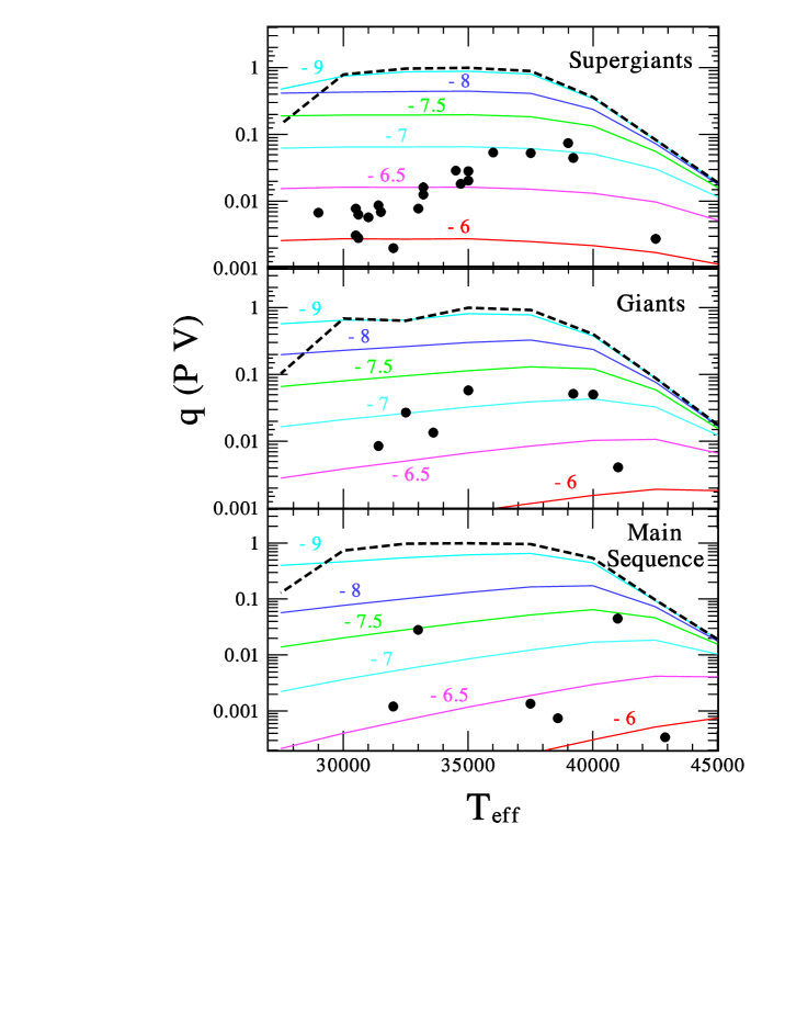
Figure 4: The effects of XUV radiation on $q$ (P v) as a function of $T_{eff}$ for different values of log ($F_{X}/F_{*}$) for the three luminosity classes. The black dashed-line represents the $\hbox{$F_{\rm X}$}=0$ case. The filled circles are the observationally determined $q$ (P v) assuming traditional $\dot{M}$ from F06 (see §3).

The predicted $q$ (P v) dependence on $F_{X}/F_{*}$ for supergiants, giants, and main sequence stars is shown in Figure 4. Also shown in this Figure are the data points from F06 that correspond to the required $q$ (P v) values if all stars have their traditional $\dot{M}$ which we will use to determine the constraints on $F_{X}/F_{*}$. This deficit in $q$ (P v) relative to unity led F06 to conclude that $\dot{M}$ needs to be reduced. Figure 4 shows a strong dependence of $q$ (P v) on $F_{X}/F_{*}$, and indicates that a range in $F_{X}/F_{*}$ between $(0.3~{}-~{}10)\times 10^{-7}$ can explain the observed $q$ (P v) for all luminosity classes. For example, from Figure 4, the observed $q$ (P v) of the four supergiants at $\hbox{$T_{eff}$}=35000$ indicate a $\hbox{$F_{X}/F_{*}$}\approx 2.5\times 10^{-7}$. This implies a XUV+X-ray flux $\approx 2\times 10^{7}$ erg cm^-2 s^-1 and a $\Delta EM_{C}$ $\approx 2.5\times 10^{29}$ cm^-5 (using Eq. 1). From X-ray analyses of OB stars we cannot directly determine $\Delta EM_{C}$ since only the volume emission measure $EM_{V}$ (cm^-3) can be deduced from observations. If we assume that the XUV+X-ray radiation arises from a spherically shell at the assumed radius ($r=1.7\hbox{$R_{*}$}$ where $\hbox{$R_{*}$}=20.5\hbox{$R_{\odot}$}$), then the “intrinsic” $EM_{V}$ is $\approx 1.8\times 10^{55}$ (using $4\pi r^{2}~{}\hbox{$\Delta EM_{C}$}$) which is comparable to the lowest energy line “observed” $EM_{V}$ ($\approx 5\times 10^{55}$ for N vii) derived from Chandra HETGS observations (e.g., Wojdowski & Schulz 2005). Since the intrinsic $EM_{V}$ is expected to be $>$ the observed $EM_{V}$ (optical depth effects), the XUV+X-ray flux required to reduce $q$ (P v) is well within the observational limits.

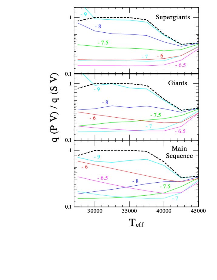
Figure 5: The ratio of $\hbox{$q$ (P {\sc v})}/\hbox{$q$ (S {\sc v})}$ as a function of $T_{eff}$ for different values of log ($F_{X}/F_{*}$) for the three luminosity classes. The black dashed-line represents the $\hbox{$F_{\rm X}$}=0$ case and this ratio is $\approx 1$ for $\hbox{$T_{eff}$}<39000$ K. See discussion in Section 3.

Now we examine the effects of XUV+X-ray radiation on S v by considering the ratio $\hbox{$q$ (P {\sc v})}/\hbox{$q$ (S {\sc v})}$. As shown in Figure 5, for the case when $\hbox{$F_{\rm X}$}=0$, this ratio is $\approx 1$ for a large range in $T_{eff}$ which supports the F06 S v surrogate argument. However, as $F_{X}/F_{*}$ increases, $\hbox{$q$ (P {\sc v})}/\hbox{$q$ (S {\sc v})}$ decreases which means that $q$ (S v) is significantly less sensitive to the XUV+X-ray radiation as compared to the dependence of $q$ (P v). This is a direct consequence of the difference in the P v and S v photoionization rates shown in Figure 3 (see §2), and invalidates the sulfur surrogate argument. In general, for all luminosity classes, $\hbox{$q$ (P {\sc v})}/\hbox{$q$ (S {\sc v})}$ reaches a minimum value of $\approx 0.14$ over most of the O-star spectral range. The required $F_{X}/F_{*}$ to produce this minimum value is dependent on luminosity class as shown in Figure 5. These results imply that the $\dot{M}$ derived from FUSE observations could be underestimated by almost an order of magnitude.

4 Discussion

We have demonstrated that the presence of XUV radiation embedded throughout a stellar wind in sufficient amounts (well within the observational constraints) can lead to a significant depletion of $q$ (P v) by using only outer shell photoionization processes. Therefore, the discrepancy between P v derived $\dot{M}$ with those obtained from density-squared diagnostics is far less severe than suggested by F06. Hence, these stars can have $\dot{M}$ that are again back within a factor of 2 range of the traditional $\dot{M}$ (consistent with clumped wind predictions). This also means that the XODUR does not require an alternative explanation.

Gudel & Naze (2009) mentioned that there may be a problem with XODUR since the wind opacities used by Waldron & Cassinelli (2007) were determined from a more highly ionized wind. Although it is true that the opacity at low energies can be sensitive to the assumed wind ionization structure, the key point is that the XODUR is based entirely on emission lines at energies $\geq$ 0.56 keV where the opacity is almost identical to the “cold” ISM opacity above this energy (e.g., see Fig. 2 of Waldron et al. 1998), and the ISM opacity represents the unsurpassable upper limit to any wind opacity. Therefore, regardless of the wind ionization state, the XODUR is certainly valid for those radii derived from the He-like $fir$ lines of Ne ix, Mg xi, Si xiii, and S xv, and radii derived from O vii may be marginally dependent on the wind ionization state.

We have shown that the inclusion of XUV radiation can resolve the $\dot{M}$ discrepancy, and there is observational support that this XUV radiation must be distributed throughout these winds based on the conclusion of M03 regarding C v. But, what is the source of this emission? Since these winds are clumped, this emission is likely to originate from bow shocks forming around clumps. The Cassinelli et al. (2008) wind bow shock model predicts that the temperature dependence of the emission measure scales as $(T/T_{max})^{-4/3}$, where $T_{max}$ is the temperature at the apex of the bow shock. Hence, there should be a considerable amount of XUV radiation, even for rather strong shocks, located at any radius. Although this XUV radiation is unobservable since essentially all of this radiation will be absorbed by the stellar wind and ISM, the strength of this emission can be determined indirectly from analyses of lower energy spectral bands as demonstrated in this paper.

Future studies now need to focus on alternate explanations as to why the X-ray lines are symmetric and nearly un-shifted. Several possibilities have been proposed: wind porosity effects (Oskinova et al. 2004, 2006); asymmetric mass outflows (Mullan & Waldron 2006), and; bow shocks forming around wind clumps (Cassinelli et al. 2008) and stellar ejected plasmoids (Waldron & Cassinelli 2009). In addition, Oskinova et al. (2007) claim that the X-ray line symmetry and P v problems can both be resolved, with no need to reduce $\dot{M}$, using their planar shock model, porosity effects, and macro-clumping. However, we argue that bow shocks will undoubtedly form around these macro-clumps and the impact of the resultant excess XUV radiation on $q$ (P v) needs to be examined. Regardless as to which explanation is applicable, our work has re-emphasized the importance of including the full XUV+X-ray energy spectrum when exploring the effects of radiation on stellar wind ionization structures.

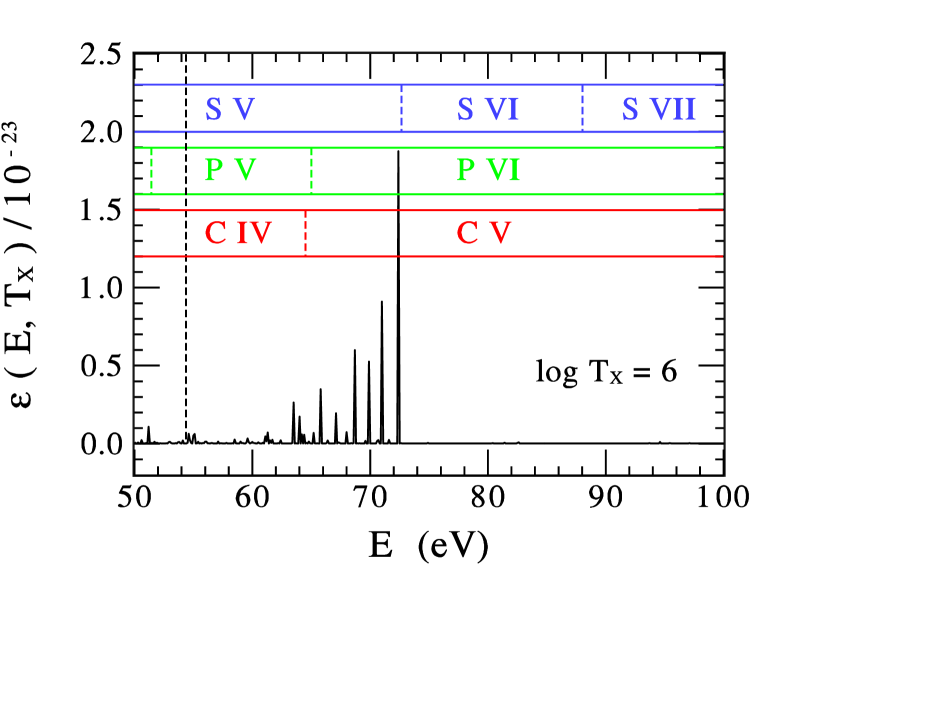
Figure 2: Comparison of the energy dependent X-ray emissivity ($\hbox{$T_{\rm X}$}=1$ MK) with the photoionization energy ranges of the relevant ions of carbon, phosphorous, and sulfur. This shows the strong collection of XUV emission lines just below the S v threshold energy at 72.68 eV, and above this energy, the XUV radiation is essentially devoid of emission lines (see §2). The four dominant XUV lines are Fe IX (72.47 eV), Fe X (71.04, 69.95 eV), and Fe XI (68.72 eV). The vertical dashed line is the He ii edge (54.4 eV).

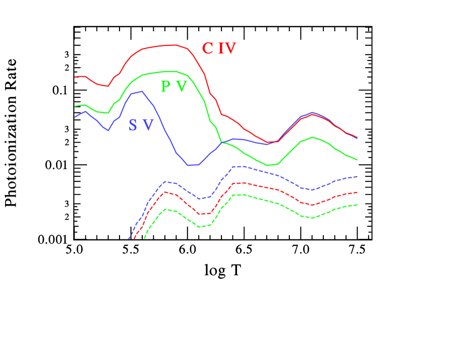
Figure 3: The XUV+X-ray photoionization rates for C iv, P v, and S v as a function of temperature assuming that $4\pi$ times the total energy integrated XUV+X-ray mean intensity above 54.4 eV is fixed at $10^{8}$ erg cm^-2 s^-1 for each temperature. The dashed-line curves show these rates as determined by using only the X-ray energy band ($\geq$ 124 eV).

References

- (1) Abbott, D. C., Bieging, J. H., & Churchwell, E. B. 1981, ApJ, 250, 645
- (2) Cassinelli, J. P., Ignace, R., Waldron, W. L., Cho, J., Murphy, N. A., & Lazarian, A.2008, ApJ, 683, 1052
- (3) Cohen, D. H., Leutenegger, M. A., Grizzard, K. T., Reed, C. L., Kramer, R. H., & Owocki, S. P. 2006, MNRAS, 368, 1905
- (4) Cox, D. P., & Tucker, W. H. 1969, ApJ, 157, 1157
- (5) Drew, J. E. 1989, ApJS, 71, 267
- (6) Fullerton, A. W., Massa, D. L., & Prinja, R. K. 2006, ApJ, 637, 1025 (FMP)
- (7) Gudel, M., & Naze, Y. 2009, A&A Rev., 17, 309
- (8) Hamann, W. -R., Feldmeier, A., & Oskinova, L. M. 2008, Clumping in Hot Star Winds, eds., W. -R. Hamann, A. Feldmeier, & L. M. Oskinova (Potsdam: Univ.-Verl.)
- (9) Hirschi, R. 2008, Clumping in Hot Star Winds, eds., W. -R. Hamann, A. Feldmeier, & L. M. Oskinova (Potsdam: Univ.-Verl.), 9
- (10) Kramer, R. H., Cohen, D. H., & Owocki, S. P. 2003, ApJ, 592, 532
- (11) Krticka, J., & Kubat, J. 2009, MNRAS, 394, 2065
- (12) Lamers, H. J. G. L. M. 1981, ApJ, 245, 593
- (13) Lanz, T., & Hubeny, I. 2003, ApJS, 146, 417
- (14) MacFarlane, J. J., Cohen, D. H., & Wang, P. 1994, ApJ, 437, 351
- (15) Martins, F., Schaerer, D., & Hillier, D. J. 2005, A&A, 436, 1049
- (16) Massa, D., Fullerton, A. W., Sonneborn, G., & Hutchings, J. B. 2003, ApJ, 586, 996 (M03)
- (17) Mewe, R., Gronenschild, E. H. B. M., & van den Oord, G. H. J. 1985, A&AS, 62, 197
- (18) Mullan, D. J., & Waldron, W. L. 2006, ApJ, 637, 506
- (19) Müller, P. E., & Vink, J. S. 2008, A&A, 492, 493
- (20) Oskinova, J., Feldmeier, A., & Hamann, W.-R. 2004, A&A, 422, 675
- (21) Oskinova, J., Feldmeier, A., & Hamann, W.-R. 2006, MNRAS, 372, 313
- (22) Oskinova, J., Hamann, W.-R., & Feldmeier, A. 2007, A&A, 476, 1331
- (23) Owocki, S. P., & Cohen, D. H. 2006, ApJ, 648, 565
- (24) Pauldrach, A. W. A., Kudritzki, R. P., Puls, J., Butler, K., & Hunsinger, J. 1994, A&A, 283, 525
- (25) Pauldrach, A. W. A., Puls, J., & Kudritzki, R. P. 1986, A&A, 164, 86
- (26) Pauldrach, A. W. A., Hoffmann, T. L., & Lennon, M. 2001, A&A, 375, 161
- (27) Puls, J., Markova, N., & Scuderi, S. 2008, ASP Conf. Ser., Mass Loss from Stars and the Evolution of Stellar Cluster, eds., A. de Koter, L. Smith, & L. Waters (San Francisco: ASP), 288, 101
- (28) Puls, J., Markova, N., Scuderi, S., Stanghellini, C., Taranova, O. G., Burnley, A. W., & Howarth, I. D. 2006, A&A, 454, 625
- (29) Puls, J., Urbaneja, M. A., Venero, R., et al. 2005, A&A, 435, 669
- (30) Smith, R. K., Brickhouse, N. S., Liedahl, D. A., & Raymond, J. C. 2001, ApJ, 556, L91
- (31) Raymond, J. C., & Smith, B. W. 1977, ApJS, 35, 419
- (32) Verner, D. A., & Yakovlev, D. G. 1995, A&AS, 109, 125
- (33) Vink, J. S., de Koter, A., & Lamers, H. J. G. L. M. 2000, A&A, 362, 295
- (34) Waldron, W. L. 1984 ApJ, 282, 256
- (35) Waldron, W. L., & Cassinelli, J. P. 2009 ApJ, 692, L76
- (36) Waldron, W. L., & Cassinelli, J. P. 2007 ApJ, 668, 456; err., 2008, ApJ, 680, 1595
- (37) Waldron, W. L., & Cassinelli, J. P. 2001 ApJ, 548, L45
- (38) Waldron, W. L., Corcoran, M. F., Drake, S. A., & Smale, A. P. 1998, ApJS, 118, 217
- (39) Withbroe, G. L., & Raymond, J. C. 1984, ApJ, 285, 347, 217
- (40) Wojdowski, P. S., & Schulz, N. S. 2005, ApJ, 627, 953