Abstract

A quantum universe with the global shape of a (Euclidean) de Sitter spacetime appears as dynamically generated background geometry in the causal dynamical triangulation (CDT) regularization of quantum gravity. We investigate the micro- and macro-geometry of this universe, using geodesic shell decompositions of spacetime. More specifically, we focus on evidence of fractality and global anisotropy, and on how they depend on the bare coupling constants of the theory.

1 Introduction

The attempt to quantize gravity using conventional quantum field theory has been gaining considerable momentum due to the progress in using renormalization group techniques [1], the understanding that one may consider an enlarged class of theories like the “Lifshitz gravity” suggested by P. Hořava [2], and by the success of nonperturbative lattice gravity theory in terms of Causal Dynamical Triangulations (CDT) in reproducing some of the infrared features of our universe from first principles [3, 4, 5, 6, 7] (see also [8] for recent reviews and [9] for a non-technical account).

The lattice approach has the potential to provide a foundation for all other, continuum-based approaches, in the same way as lattice field theory serves as an underlying non-perturbative definition of continuum quantum field theories, as emphasized by K. Wilson. The lattice formulation is based on piecewise linear geometries, which require no coordinate systems: all geometric information is contained in tables listing elements in the immediate neighbourhood of a given (sub-)simplex and length/volume assignments for specific (sub-)simplices. This provides an explicit realization of the relational nature of aspects of pure spacetime geometry, familiar from the classical theory of General Relativity.

While getting rid of coordinates and the redundancy associated with the arbitrariness of a coordinate choice is highly attractive from a conceptual point of view, it comes with a unique set of challenges when one tries to extract information about the quantum geometry. The well-known problem of identifying invariantly defined gravitational observables is aggravated in the quantum theory, where in addition one has to consider expectation values, that is, averages over all geometries. If instead one wanted to work with individual path integral configurations, which do have a definite geometry, great care has to be taken in interpreting them since they are not physical, in the same way as an individual path in the path integral of the particle is not an observable. Moreover, the typical configurations in a quantum field theory which is not topological are dominated by ultraviolet fluctuations, making it rather subtle to extract physical information from them.

In this letter we will define and measure a number of “quantum observables” to quantify further the geometric properties of the quantum de Sitter universe to emerge from nonperturbative lattice simulations of quantum gravity in terms of causal dynamical triangulations. Building on previous results presented in [4, 6, 7], the quantities we will consider characterize the fractality of the spacetime as a whole and of certain hypersurfaces inside it, as well as potential global anisotropies between the time and space directions of the quantum universe.

2 The macroscopic $S^{4}$-universe

In practice, the nonperturbative and background-independent quantization of gravity in CDT proceeds via Monte Carlo simulations, which generate a sequence of piecewise flat spacetime geometries from the following input: (i) a choice of global spacetime topology, usually $S^{3}\times S^{1}$, (ii) the Einstein-Hilbert action, which has a natural implementation on piecewise linear geometries, (iii) a specific form of the piecewise linear, Minkowskian building blocks, the four-simplices to be glued together, (iv) a global proper-time foliation for each path integral history, and, finally, (v) a rotation to Euclidean time of each path integral configuration (see [4] for technical descriptions of all of the above). On the output side, we observe the emergence of a background geometry, with well-defined quantum fluctuations around it, whose large-scale shape has been matched with great accuracy to that of a “round $S^{4}$”, a (Euclidean) de Sitter universe, see [7] for details.

This is a result which is (a) non-trivial, and (b) not universally true. It is non-trivial because the four-sphere is only a saddle point solution to the Euclidean equations and there is no obvious reason why it should dominate the path integral, in particular, since the action is unbounded from below. This means that the appearance of $S^{4}$ is due to a subtle interplay between the entropy of configurations (the path integral measure) and the bare action. This is also the reason why the result is not universally true: only in a certain range of bare coupling constants will the $S^{4}$-like background dominate. It is the geometries in this so-called “phase C” [4] whose properties we will investigate presently. For other values of the bare coupling constants one finds other phases (called $A$ and $B$ in [4]), and phase transitions between them. We not in passing that the phase diagram of CDT quantum gravity bears an intriguing resemblance to that of Lifshitz gravity, as discussed in some detail in [10], and is the subject of ongoing research.

The Euclidean Einstein action and its implementation on piecewise linear geometries are given by

$$S_{E} = \frac{1}{16\pi^{2}G}\int\sqrt{g}(-R+2\Lambda)$$ (1)

$$\to -(\kappa_{0}+6\Delta)N_{0}+\kappa_{4}(N_{4}^{(4,1)}+N_{4}^{(3,2)})+\Delta(2N_{4}^{(4,1)}+N_{4}^{(3,2)}),$$

where $N_{0}$ is the number of vertices, $N_{4}^{(4,1)}$ the number of four-simplices with four vertices in one spatial slice and one vertex in one of the adjacent spatial slices, and $N_{4}^{(3,2)}$ the number of four-simplices with three vertices in one spatial slice and two vertices in a neighbouring slice. The coupling $\kappa_{0}$ is proportional to the inverse bare gravitational coupling constant, while $\kappa_{4}$ is linearly related to the bare cosmological coupling constant. Finally, $\Delta$ is an asymmetry parameter related to the fact that we allow for a finite relative scaling between the length of space- and time-like links. The reason why the simplicial form of the action is so simple is that all building blocks of type (4,1) and all building blocks of type (3,2) are identical.

Since for simulation-technical reasons it is preferable to keep the total four-volume fixed during the Monte Carlo simulation, $\kappa_{4}$ effectively does not appear as a coupling constant. Instead, one can perform simulations for different four-volumes. This leaves us with two bare coupling constants, $\kappa_{0}$ and $\Delta$. We start out with $(\kappa_{0},\Delta)=(2.2,0.6)$, a value firmly placed in phase $C$, at which most of our previous computer simulations were performed. For this “generic” value we have shown that by a suitable global rescaling of the continuum proper time, the extended quantum universe can be viewed as a standard round four-sphere with superimposed quantum fluctuations [6, 7]. We also reported in [7] that the overall shape of the background universe can change as a function of the bare coupling constants. In other words, to map the dynamically generated quantum universe at generic points in phase $C$ to a $S^{4}$ requires a coupling constant-dependent rescaling of “time” with respect to “space”.

In this article we are mainly interested in the changes that occur when one decreases $\Delta$. The reason is that in this manner one approaches the phase transition between phases C and B, which is a potential candidate for a second-order transition line. To give a first indication of what happens, we have measured the change in shape, by which we shall mean the average volume profile $\langle V_{4}(t)\rangle$ as a function of the lattice proper time $t$, where $V_{4}(t)$ denotes the (discrete) four-volume ($=$number of four-simplices) located in the spacetime slab between times $t$ and $t+1$. Fig. 1 illustrates how the universe’s extension in the time direction, measured in units of discrete lattice steps, becomes shorter when we decreas $\Delta$ from 0.6 to 0.1. Our main aim in the present work is to describe the geometry of CDT’s quantum universe in greater quantitative detail, both at the generic point and when changing $\Delta$.

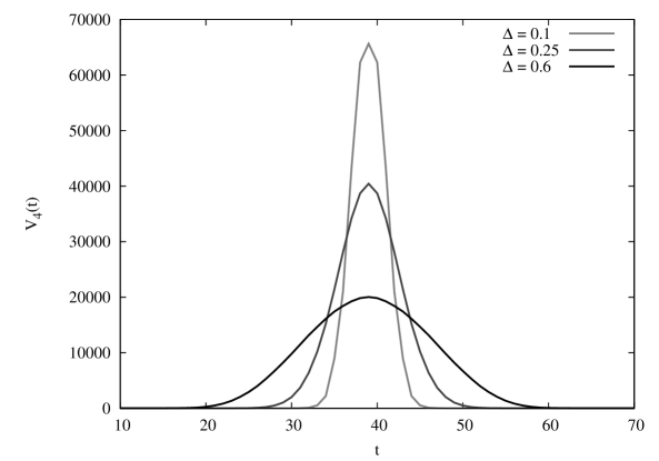
Figure 1: The volume profile $\langle V_{4}(t)\rangle$ for decreasing values of the asymmetry $\Delta$ = 0.6, 0.25 and 0.1, with total four-volume kept constant. The profile narrows as $\Delta$ decreases.

3 Exploring the universe by shell decomposition

To study the invariant properties of geometry we move along geodesics, which in the Euclideanized, piecewise linear context we define as the shortest piecewise straight paths between any two centres of four-simplices, where each path consists of a sequence of straight segments connecting the centres of neighbouring four-simplices. The length of a path is simply taken as the number of “hops” between adjacent four-simplices. We could in principle work with a finer-grained definition, for example, by using some notion of geodesic on the piecewise linear geometry, which is defined between any pair of points. However, there is no reason for the details of a piecewise linear geometry of an individual triangulation to be of interest at the very shortest distances, where they are clearly an artifact of the specific choice of building blocks made. We expect that our simple definition of a geodesic will in the continuum limit (that is, on scales sufficiently large compared to the cut-off scale) lead to the same geometric results as other “reasonable” definitions. Note that our way of implementing geodesics does not distinguish between segments in space and time direction; we will return in later sections to the issue of relative scaling between spatial and time distances.

The way we will make use of geodesics in the present article is by propagating either from a point or a given hypersurface in discrete geodesic steps of unit length to consecutive geodesic shells, foliating part or all of the universe. We collect certain data associated with such shell decompositions, from which we reconstruct the following geometric information about the quantum universe: (i) its fractal structure, (ii) its average volume distribution as function of time and spatial distance, and (iii) an estimate of its global shape. While (ii) and (iii) refer to genuine averages over many configurations, measurements relating to (i) will make use of individual configurations in the way described below.

Let us describe some key elements of our measurement process. For any fixed, given universe configuration generated by the Monte Carlo simulation, we first locate its (non-unique) “centre”, defined as any four-simplex lying in the spacetime slab with maximal volume $V_{4}(t)$, whose time label we will denote by $t_{0}$. Picking an arbitrary four-simplex in this maximal slab, we move outwards from this centre in spherical shells (in a four-dimensional sense), advancing in geodesic steps of length 1. We record various pieces of information on the way, most prominently, the four-volume $V_{4}(t,r)$ in the shell of four-simplices located a distance of $r$ steps away from the centre and at the same time located in time slab $t$. Thus $V_{4}(t,r)$ constitutes a fraction of both $V_{4}(t)$ and of $\tilde{V}_{4}(r)$, which by definition is the four-volume of the entire shell (i.e. the number of four-simplices contained in it) at distance $r$. Summarizing the situation, we have the relations

$$V_{4}(t)=\sum_{r}V_{4}(t,r)$$ (2)

and

$$\tilde{V}_{4}(r)=\sum_{t}V_{4}(t,r),$$ (3)

as well as

$$V_{4}=\sum_{t}V_{4}(t)\equiv\sum_{r}\tilde{V}_{4}(r)$$ (4)

for the total four-volume $V_{4}$. In order to be able to average over many configurations we redefine our time labeling such that $t_{0}$ always corresponds to time zero. For investigating the fractal nature of an individual spacetime configuration (its “branchedness” and possible associated self-similarity), we also record the connectivity of the shell at distance $r$, where two simplices in the shell at distance $r$ are called connected if one can find a path connecting them using simplices only from shells with some larger distance $r^{\prime}\geq r$.

4 The results

4.1 The fractal structure

We have measured the fractal structure of individual path-integral histories for a number of different values of $\Delta$, starting at $\Delta=0.6$ and ending at $\Delta=0.06$ (with $\kappa_{0}=2.2$ understood), with Fig. 2 giving a representative sample of data.

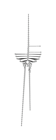
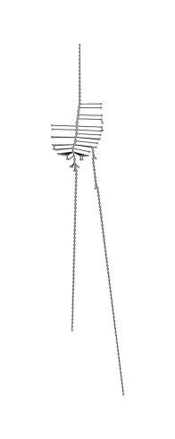
Figure 2: Tree graphs illustrating the connectedness of radial shells, starting from a central four-simplex of a spacetime configuration (top node of graph) and moving outward in discrete, concentric spherical shells (corresponding to going down or sideways in the tree graph). From left to right, measurements taken at $\Delta$= 0.06, 0.25 and 0.6.

The figures should be read as follows: the top node of each of the three tree graphs represents the chosen “centre of the universe”, and distance from the centre increases as one moves down or sideways in the graph. Each node represents a connected component of a shell. A line connecting two nodes indicates that there is a four-simplex in one of the connected components which is a direct neighbour of a four-simplex in a connected component in a neighbouring shell. By construction, such a graph will be a tree graph. One might call it a diffusion tree, since one essentially follows the front of the simplest diffusion process one can study on a given configuration. The size of a node is a measure of the number of four-simplices in the associated connected component of the shell. To optimize the graphical presentation, the radius $\rho$ of the node has been chosen as $\rho\propto V_{4}^{1/10}$, and only shells (and sub-shells) with more than 40 simplices have been included.

The qualitative features of the graphs shown in Fig. 2 are generic and there is little sign of any nontrivial branching structure. One typically finds one sequence of connected shells which dominates (some small disconnected components are created but end almost immediately), which at some point bifurcates into two. The figure also illustrates that this bifurcation becomes more pronounced for larger $\Delta$. The interpretation of this phenomenon in terms of the overall shape of the quantum universe should be clear: for large $\Delta$ we have a four-sphere which has been stretched along the time direction. The analogue in two dimensions lower would be that of a round two-sphere stretched along one of its directions to create a prolate spheroid (the surface of revolution obtained by rotating an ellipse about its major axis). Starting a diffusion process from any point along the equator along the nonstretched direction, the diffusion front will propagate in concentric circles until it meets itself at the antipode of the starting point, where it will then bifurcate and move in opposite directions toward the pointed ends of the spheroid. Returning to the case of four dimensions, the spheroid becomes more spherical with decreasing $\Delta$, and consequently the bifurcation becomes less pronounced (and even disappears for the lowest value of $\Delta$), as we have been observing. Although our discussion of fractal behaviour above is of a qualitative nature, it is reasonably straightforward to construct related quantum observables whose expectation value on the ensemble of all spacetimes is well defined and can be measured quantitatively. An example of this is the “sphericity” of the universe, which will be introduced in Sec. 4.3 below.

4.2 The volume of shells

The picture of a diffusion process on a spheroid is corroborated by measurements of $V_{4}(t,r)$ for various values of $\Delta$. Unlike in the previous section, the data collected do not refer to a single configuration, but to a combined average over configurations and initial points (where for each given spacetime configuration, we selected 100 different starting points in the maximal time slab and repeated the diffusion process).

In Fig. 3 we show contour plots of the distribution $V_{4}(t,r)$ for various $\Delta$, which for large $\Delta$ assume a characteristic “V”-shape in the $t$-$r$-plane. They indicate that the diffusion front splits into two after a certain distance $r_{bif}$, called the bifurcation distance, which should be identified with half the length of the equator of the (unstretched, round) three-sphere at time $t_{0}$.

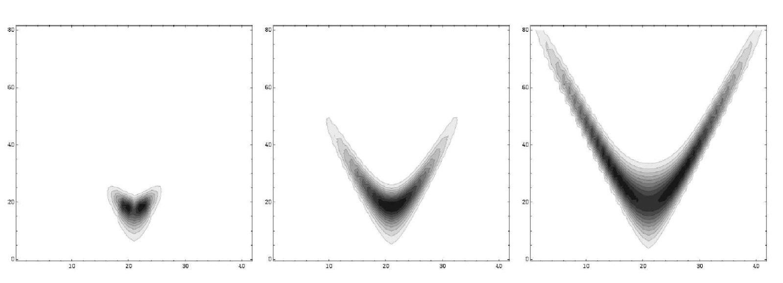
Figure 3: Contour plots of the distribution $V_{4}(t,r)$, as function of the spacetime slab $t$ (horizontal axes) and the distance $r$ travelled by the diffusion front (vertical axes) from its initial point. The processes are centred in slice $t_{0}=20$, and the plots are taken at $\Delta$ = 0.06, 0.25 and 0.6 (left to right).

As $\Delta$ decreases the V-shape diminishes, with the obvious interpretation that the shape of the spheroid becomes more and more spherical, with approximately equal extension in spatial and time directions.

Additional evidence for this geometric interpretation comes from starting the diffusion instead at one of the tips of the spheroid. In this case one never observes any V-shape, and the front of diffusion is not very different from the proper-time slicing which was used to define the original global time in the computer simulations.

A related study has recently been performed in three-dimensional CDT, using the full diffusion equation [14] and comparing it with the diffusion on an elongated sphere. The conclusion was that from the point of view of long-distance diffusion one can indeed view the quantum geometry in the three-dimensional case as that of a stretched sphere with small superimposed quantum fluctuations. In the four-dimensional case we have one more coupling constant at our disposal, the asymmetry factor $\Delta$, which seemingly allows us to monitor the shape of the universe when described in terms of lattice spacings. However, the conclusion that the real quantum universe changes shape under a change in $\Delta$ may be premature: as we will explain further in Sec. 6, when discussing the situation in terms of actual physical distances (instead of just lattice units), the shape of the universe may actually change very little or even not at all.

4.3 The function $\tilde{V}_{4}(r)$ and sphericity

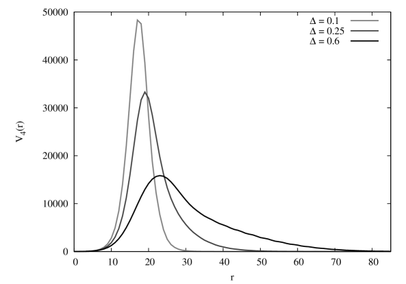
Figure 4: Average radial volume distribution $\tilde{V}_{4}(r)$ as function of the distance $r$ from a “centre of the universe”.

Next we turn to the distribution of the number $\tilde{V}_{4}(r)$ of four-simplices in a shell at distance $r$ from a given centre of the universe, as defined in Sec. 3 above. Fig. 4 shows $\tilde{V}_{4}(r)$ for various values of $\Delta$. For the smallest values of $\Delta$ the peak is nicely symmetric and well approximated by $A\sin^{3}(r/B)$, in agreement with earlier studies of the curve $V_{4}(t)$. The hypersurfaces of constant radius $r$ are of course completely different from those of constant $t$, but nevertheless it turns out that $\tilde{V}_{4}(r)$ agrees with $V_{4}(t)$ up to a rescaling of the constants. For larger values of $\Delta$ the situation is different in that $\tilde{V}_{4}(r)$ has a large-$r$ tail, which cannot be fitted to $A\sin^{3}(r/B)$. This behaviour is again consistent with universes of the form of prolate spheroids: for a genuinely spherical configuration, $\tilde{V}_{4}(r)$ would vanish for radii $r$ larger than the distance between antipodal points. By contrast, for elongated configurations the diffusion front bifurcates when the antipodal point is reached, and continues further towards the tips of the spheroid.

Let us try to quantify how spherical our averaged configuration is by defining the sphericity $s$ by

$$s:=\frac{\sum_{r=0}^{r_{bif}}\tilde{V}_{4}(r)}{\sum_{r=0}^{r_{max}}\tilde{V}_{4}(r)}.$$ (5)

In agreement with our earlier characterization, $r_{bif}$ is defined operationally as the largest radius $r$ for which $V_{4}(t_{0},r)$ is larger than some cut-off, here taken to be 4 (recall that $t_{0}$ marks the spacetime slice of maximal four-volume). Similarly, $r_{max}$ is the largest distance $r$ for which $\tilde{V}_{4}(r)$ is larger than the cut-off. This implies that the denominator of the quotient (5) is an overall normalization, given by the total four-volume minus the volume of the “stalk” (where the spatial universe only persists because we do not allow it to shrink to zero volume). Fig. 5 shows how $s$, averaged over both configurations and initial points, depends on $\Delta$. From comparing with the diffusion trees one would expect $s$ to be close to 1 for the smallest values of $\Delta$ considered here. This is indeed what we find confirmed here. Of course, $s=1$ is exactly the value which we would also obtain for a round sphere in the continuum.

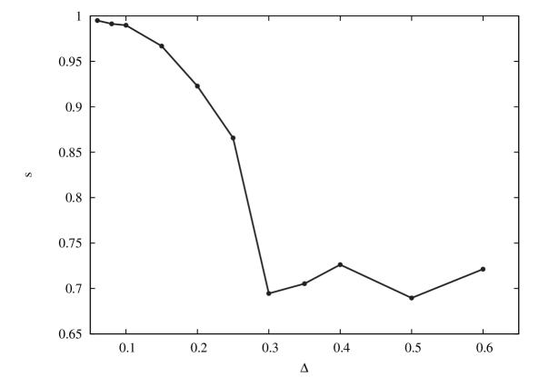
Figure 5: Sphericity $s$ of the quantum universe for different values of the asymmetry parameter $\Delta$.

5 The fractal structure of spatial slices

When studying the connected components of a shell at distance $r$ above, the connectivity was defined in a four-dimensional sense, in that the connecting paths were allowed to lie not only in the shell $r$, but also in shells with $r^{\prime}>r$. The resulting tree structure did not exhibit any fractality. This picture changes drastically when we confine ourselves to a shell at fixed $r$ and define connectivity with respect to paths that lie entirely within that shell. What we have found is that the structure of the shells at fixed radius $r$ is quantitatively similar to both that of the four-dimensional time slabs labeled by time $t$, as well as that of the three-dimensional hypersurfaces at constant time $t$, made exclusively from spatial tetrahedra. Since the spatial hypersurfaces at fixed time $t$ are the easiest to handle numerically, we have used them to collect our data set. What we would like to emphasize is that the structure reported below is equally valid for any of the hypersurfaces or slabs appearing above, and presumably reflects the properties of generic (reasonably chosen) hypersurfaces.

A hypersurface of this kind is a three-dimensional triangulation, more precisely, a piecewise linear manifold of topology $S^{3}$. The mismatch between the measured values of its spectral dimension, $d_{S}\approx 1.5$, and its Hausdorff dimension, $d_{H}\approx 3$, is an indicator of the nonclassical, fractal nature of these slices (for definitions and results, see [4]). We will now quantify their fractality in a more direct way, with the tree structure defined in terms of so-called “minimal necks” [15, 16]. Such a minimal neck consists of four neighbouring triangles which are glued together in such a way as to form a minimal representation of a topological two-sphere, or, equivalently, the surface of a solid tetrahedron, but without the interior of the tetrahedron forming part of the three-dimensional triangulation.

Cutting a triangulation along a minimal neck will separate it into two disconnected parts which can both be made into triangulations of $S^{3}$ by closing off the two boundaries, each given by a copy of the minimal neck, with two tetrahedral building blocks. Cutting along each minimal neck in the triangulation and repeating the process leaves us with a number of $S^{3}$-components. Each of these we represent by a graph vertex, which is then reconnected by a graph edge to each vertex representing a $S^{3}$-component that was originally connected to the first one by a minimal neck. By this “minimal-neck surgery” we can associate a unique tree graph to any three-dimensional triangulation. Fig. 6 illustrates a typical tree structure associated with a given triangulated hypersurface.

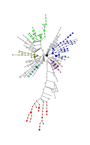
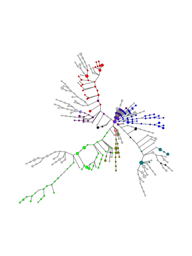
Figure 6: The fractal structure of two neighbouring hypersurfaces at times $t$ and $t+1$, using the tree structure induced by minimal necks. Matching colours signify neighbouring vertices in the adjacent hypersurfaces, as explained in the text.

The resulting tree structure reflects a rough three-dimensional distance hierarchy, but does this persist in a four-dimensional sense once we re-allow for paths which can leave the hypersurface, and may lead to short-cuts between points on it? To some extent it does, at least in a statistical sense. Namely, we have checked that typical distances between pairs of points are not drastically altered when considering the full, four-dimensional embedding. The observed fractal structure is therefore not entirely an artifact of defining a hypersurface in a generic spacetime configuration appearing in the path integral, which of course is subject to wild ultraviolet fluctuations.

There is another type of measurement we have made to corroborate the persistence of the fractal structure when going from one hypersurface to the next. In order to compare the tree structures at times $t$ and $t+1$, we define a neighbourhood relation as follows. For a given tetrahedron belonging to a vertex in the constant-time slice at $t$, its “neighbours” in time slice $t+1$ are the tetrahedra which are at a (four-dimensional) distance 4 away from it. Two $S^{3}$-components represented by vertices $v$ and $v^{\prime}$ at times $t$ and $t+1$ are neighbours if the minimal distance between pairs of tetrahedra $(\tau,\tau^{\prime})$, $\tau\in v$, $\tau^{\prime}\in v^{\prime}$, is 4. One can now study whether this nearest-neighbour association between components (vertices) has any relation with the tree structure defined a priori at time $t+1$. For purposes of illustration we have marked all vertices of a given tree branch at time $t$ in a chosen colour. For each vertex we then find its neighbouring vertices in time slice $t+1$, and mark them with the same colour, allowing also for mixing of colours.

An example of the coloured connectivity trees of two adjacent slices is given in Fig. 6, where one should keep in mind that the only relevant feature conveyed is the connectivity along the edges of the graph, and not the location of the vertices in the two-dimensional plane. The resemblance of the two coloured graphs shows clearly that the associated fractal structures of the hypersurfaces are correlated, and not totally independent of each other. In principle one can try to establish similar relations between slices that are two or more steps apart, by using “neighbours of neighbours”, but this notion of neighbourhood soon becomes rather weak. – As usual in discussions of local correlations of this type in the context of nonperturbative, “background-free” quantum gravity, it is a challenge to define suitable observables to convert statements like the above to more quantitative ones, a line of enquiry we shall take up elsewhere.

6 Discussion

The CDT prescription for constructing a theory of quantum gravity is extremely simple, namely, as the path integral over causal spacetime geometries with a global time foliation. In order to perform this summation explicitly, one introduces a grid of piecewise linear geometries, in much the same way as when defining the path integral in quantum mechanics. The action used is the Einstein-Hilbert action in the form of the Regge action for piecewise linear geometries. Next, one rotates each of the Lorentzian geometries to Euclidean signature, and performs the path integral with the help of Monte Carlo simulations, thus restricting one to stay in the Euclidean sector. The key outcome is that in a certain range of bare coupling constants (“phase C”) one observes a quantum universe which can be described as an emergent four-dimensional cosmological “background” geometry with superimposed quantum fluctuations, and a highly nonclassical short-distance behaviour, as reflected in an anomalous spectral dimension, $d_{s}\approx 2$, and some evidence of fractality.

What is somewhat unusual compared to the standard lattice scenario is that the nontrivial infrared behaviour is observed for a whole range of coupling constants. The purpose of this article was to have a closer look at the geometric properties of the quantum universe in this phase C, using various geodesic shell decompositions. We were specifically interested in gathering further evidence for the presence or otherwise of fractal features and in how these and some global shape variables are influenced by a change in the asymmetry parameter $\Delta$, which together with the bare Newton’s constant parametrizes the phase space of the underlying statistical model. In previous work we have shown that for a specific choice of bare coupling constants in phase C (generic in the sense of not being close to any phase transitions) one can by a finite, global rescaling of the continuum cosmological proper time map the expectation value of the volume profile of the quantum universe to that of a round four-sphere, that is, Euclidean de Sitter space. Does this picture change when we change the values of the bare coupling constants?

In this paper, we have left the bare inverse gravitational constant unchanged and varied the coupling constant $\Delta$ between the generic value $\Delta=0.6$ used previously and (almost) zero. We cannot go all the way to zero because there is a phase transition just before we reach zero, and close to it our current Monte Carlo sampling becomes ineffective. On the face of it, most of our results show a clear $\Delta$-dependence, as illustrated by Figs. 1–5. Only for small $\Delta$, corresponding to $\alpha\approx 1$ are our results compatible with a truly spherical universe. Is this in contradiction with earlier claims that we observe a de Sitter universe throughout phase C? Not necessarily: as we have already alluded to in Sec. 4.2, it may be that continuum physics is invariant under a variation in $\Delta$, at least as long as we stay away from the phase transition.

Let us present some evidence that our current data is not in disagreement with such a hypothesis. The key point is that $\Delta$, which appears linearly in the action (1) can be viewed as a choice of asymmetry between space and time [4]. A more direct measure of this asymmetry is given by the parameter $\alpha$, introduced originally in [17, 13] as the proportionality factor between the (squared) length of time- and spacelike edges, $a_{t}$ and $a_{s}$, according to $a_{t}^{2}=\alpha a_{s}^{2}$. Now, considering the relation between $\alpha$ and $\Delta$, plotted in Fig. 7, one observes that a decrease in $\Delta$ is associated with an increase in $\alpha$. In other words, a lattice unit in time direction corresponds to an ever larger physical distance as $\Delta\rightarrow 0$. When taking this effect into account – as one should – when considering the shape of the universe or the distribution $V_{4}(t,r)$, say, one sees that it could potentially compensate for the differences for different $\Delta$ which we observed when expressing our results in terms of fixed lattice units. This would imply that the “true” physics is unchanged under variation of either $\alpha$ or $\Delta$ throughout phase C. The region where true sphericity is realized appears to be for $\alpha\approx 1$. This also happens to be the region where the spatial diameter and the time extent, when measured in terms of discrete lattice units, are approximately equal.

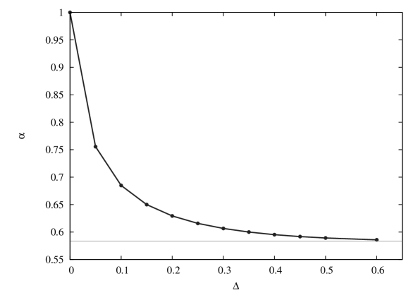
Figure 7: The asymmetry factor $\alpha$, plotted as a function of $\Delta$, for $\kappa_{0}=2.2$. The horizontal line is $\alpha=7/12$, the lowest kinematically allowed value of $\alpha$, where the (3,2)-simplices degenerate because of a saturation of a triangle inequality [13].

It is difficult to convert this argument into a more quantitative statement about the shape of the spheroid, say, because we do not at this stage have an independent way (other than fitting the quantum universe to the round four-sphere) of establishing the relative scaling between time and spatial distances in the continuum theory. The regularized theory is ambiguous when it comes to defining something like the “timelike distance between spatial slices”, not least because of the singular nature of the piecewise flat geometries. The easiest definition is to take it to be unity in terms of discrete lattice units, as is usually done. Alternatively, one could again take the local, piecewise flat geometry literally and work out the true geodesic distance of a point $x$ in the spatial slice at time $t+1$ to the previous slice at time $t$ (which would lead one to conclude that as a result of the specific geometry of the simplices and how they are glued together, this distance can vary between $c_{1}a_{s}$ and $c_{2}a_{s}$, where $c_{1},c_{2}$ are constants which themselves depend on $\alpha$). Of course, this distance would also on average decrease when decreasing $\alpha$, but would be distinct from the “step distance” at the cut-off scale. Nevertheless, one’s expectation would be that different definitions of discrete distance will give rise to equivalent notions of “continuum distance”, which differ at most by a global rescaling. However, it was exactly this relative global scale we were trying to determine above.

In summary, our hypothesis that continuum physics and geometry do not change as the asymmetry parameter is changed continuously is not contradicted by present measurements, but further corroboration will have to await the study of finer-grained observables, which can distinguish spheroids from true spheres. This also points to a potential flaw in the way we have defined some of our “observables”, like those depicted in Figs. 1–5. In their definition, we simply treated time and space directions on an equal footing (for example, when advancing shells in unit steps from a given point). This can create a spurious $\Delta$-dependence. For example, if our hypothesis is correct and the universe is a round four-sphere, no matter where we are in phase C, one would say that graphs like those for $\Delta=0.25$ and $\Delta=0.6$ in Fig. 2 cannot be counted as evidence for the presence of global anisotropy.

Once we cross the phase transition line and enter phase B, the situation changes dramatically and there remains only a single time slice which has a spatial three-volume different from the minimal cut-off value – four-dimensional spacetime has completely disappeared! Presently it is unclear whether this happens abruptly (corresponding to a first-order transition) or merely fast but smoothly (corresponding to a second-order transition). If the latter was the case, it would probably be inconsistent to maintain that the physical shape remained unchanged all the way to the transition line. On the other hand, other scenarios may then suggest themselves, involving perhaps an asymmetric scaling of space and time along the lines envisaged in Hořava-Lifshitz gravity, see also [10].

Lastly, to return to the other one of our main themes, that of fractality, our more detailed investigation finds little or no evidence of fractality when looking at a shell decomposition of spacetime. By contrast, when performing a shell decomposition within a given hypersurface (a shell or slice of constant $r$ or $t$), we have confirmed earlier findings of a fractal structure [4] for hypersurfaces of constant proper time and have verified that they are also present for more general types of shells. We have gone one step further and found (at least qualitative) evidence that the fractal structure of the hypersurface is propagated to a neighbouring one, which means that it is not entirely an artifact confined to a single, isolated shell. We do not yet understand the ramifications of this result for the short-scale physics of the quantum universe. Most likely it is related to the anomalous spectral dimension observed in [18] and obtained in both the asymptotic safety scenario [19] and Hořava-Lifshitz gravity [20]. It would be interesting if this could be understood in more detail.

Acknowledgements. JA and RL are grateful to the Perimeter Institute for hospitality. JJ acknowledges partial support through grant 182/N-QGG/2008/0 “Quantum geometry and quantum gravity”, financed by the Polish Ministry of Science. AG has been supported by the Polish Ministry of Science grants N N202 034236 (2009-2010) and N N202 229137 (2009-2012). RL acknowledges support by the Netherlands Organisation for Scientific Research (NWO) under their VICI program.

References

-
[1]
A. Codello, R. Percacci and C. Rahmede:
Investigating the ultraviolet properties of gravity with a Wilsonian
renormalization group equation,
Annals Phys. 324 (2009) 414-469
[arXiv:0805.2909, hep-th];
M. Reuter and F. Saueressig: Functional renormalization group equations, asymptotic safety, and Quantum Einstein Gravity, Lectures given at First Quantum Geometry and Quantum Gravity School, Zakopane, Poland, 23 Mar - 3 Apr 2007, 57 pages [arXiv:0708.1317, hep-th];
M. Niedermaier and M. Reuter: The asymptotic safety scenario in quantum gravity, Living Rev. Rel. 9 (2006) 5, 173 pages;
H.W. Hamber and R.M. Williams: Nonlocal effective gravitational field equations and the running of Newton’s G, Phys. Rev. D 72 (2005) 044026, 16 pages [hep-th/0507017];
D.F. Litim: Fixed points of quantum gravity, Phys. Rev. Lett. 92 (2004) 201301, 4 pages [hep-th/0312114];
H. Kawai, Y. Kitazawa and M. Ninomiya: Renormalizability of quantum gravity near two dimensions, Nucl. Phys. B 467 (1996) 313-331 [hep-th/9511217]. - [2] P. Hořava: Quantum gravity at a Lifshitz point, Phys. Rev. D 79 (2009) 084008 [arXiv:0901.3775, hep-th].
- [3] J. Ambjørn, J. Jurkiewicz and R. Loll: Emergence of a 4D world from causal quantum gravity, Phys. Rev. Lett. 93 (2004) 131301, 4 pages [hep-th/0404156].
- [4] J. Ambjørn, J. Jurkiewicz and R. Loll: Reconstructing the universe, Phys. Rev. D 72 (2005) 064014, 24 pages [hep-th/0505154].
- [5] J. Ambjørn, J. Jurkiewicz and R. Loll: Semiclassical universe from first principles, Phys. Lett. B 607 (2005) 205-213 [hep-th/0411152].
- [6] J. Ambjørn, A. Görlich, J. Jurkiewicz and R. Loll: Planckian birth of the quantum de Sitter universe, Phys. Rev. Lett. 100 (2008) 091304, 4 pages [arXiv:0712.2485, hep-th].
- [7] J. Ambjørn, A. Görlich, J. Jurkiewicz and R. Loll: The nonperturbative quantum de Sitter universe, Phys. Rev. D 78 (2008) 063544, 17 pages [arXiv:0807.4481, hep-th].
-
[8]
J. Ambjørn, J. Jurkiewicz and R. Loll:
Causal dynamical triangulations and the quest for quantum gravity,
to appear in “Foundations of space and time”, eds. G. Ellis, J. Murugan and
A. Weltman, Cambridge Univ. Press [arXiv:1004.0352, hep-th];
Quantum gravity as sum over spacetimes, to appear in
“Quantum Gravity - New Paths Towards Unification”, Springer
Lecture Notes in Physics [arXiv:0906.3947, gr-qc];
R. Loll: The emergence of spacetime, or, quantum gravity on your desktop, Class. Quant. Grav. 25 (2008) 114006 [arXiv:0711.0273, gr-qc]. - [9] J. Ambjørn, J. Jurkiewicz and R. Loll: The universe from scratch, Contemp. Phys. 47 (2006) 103-117 [hep-th/0509010].
- [10] J. Ambjørn, A. Görlich, S. Jordan, J. Jurkiewicz and R. Loll: CDT meets Hořava-Lifshitz gravity [arXiv:1002.3298, hep-th].
-
[11]
J. Ambjørn, J. Jurkiewicz and Y. Watabiki:
On the fractal structure of two-dimensional quantum gravity,
Nucl. Phys. B 454 (1995) 313-342 [hep-lat/9507014];
J. Ambjørn and K.N. Anagnostopoulos: Quantum geometry of 2D gravity coupled to unitary matter, Nucl. Phys. B 497 (1997) 445-478 [hep-lat/9701006]. - [12] J. Ambjørn, J. Jurkiewicz and R. Loll: Non-perturbative 3d Lorentzian quantum gravity, Phys. Rev. D 64 (2001) 044011 [hep-th/0011276].
- [13] J. Ambjørn, J. Jurkiewicz and R. Loll: Dynamically triangulating Lorentzian quantum gravity, Nucl. Phys. B 610 (2001) 347 [hep-th/0105267].
- [14] D. Benedetti and J. Henson: Spectral geometry as a probe of quantum spacetime, Phys. Rev. D 80 (2009) 124036 [arXiv:0911.0401, hep-th].
- [15] J. Ambjørn, S. Jain and G. Thorleifsson: Baby universes in 2-d quantum gravity, Phys. Lett. B 307 (1993) 34 [hep-th/9303149].
- [16] J. Ambjørn, S. Jain, J. Jurkiewicz and C.F. Kristjansen: Observing 4-d baby universes in quantum gravity, Phys. Lett. B 305 (1993) 208 [hep-th/9303041].
- [17] J. Ambjørn, J. Jurkiewicz and R. Loll: A non-perturbative Lorentzian path integral for gravity, Phys. Rev. Lett. 85 (2000) 924 [hep-th/0002050].
- [18] J. Ambjørn, J. Jurkiewicz and R. Loll: Spectral dimension of the universe, Phys. Rev. Lett. 95 (2005) 171301 [hep-th/0505113].
- [19] O. Lauscher and M. Reuter: Fractal spacetime structure in asymptotically safe gravity, JHEP 0510 (2005) 050 [hep-th/0508202].
- [20] P. Hořava: Spectral dimension of the universe in quantum gravity at a Lifshitz point, Phys. Rev. Lett. 102 (2009) 161301 [arXiv:0902.3657, hep-th].