The Belle Collaboration

 
Search for $B^{0}\to K^{*0}\overline{K}{}^{*0}$, $B^{0}\to K^{*0}K^{*0}$ and $B^{0}\to K^{+}\pi^{-}K^{\mp}\pi^{\pm}$ Decays

Abstract

We report a search for the decays $B^{0}\to K^{*0}\overline{K}{}^{*0}$ and $B^{0}\to K^{*0}K^{*0}$. We also measure other charmless decay modes with $K^{+}\pi^{-}K^{-}\pi^{+}$ and $K^{+}\pi^{-}K^{+}\pi^{-}$ final states. The results are obtained from a data sample containing $657\times 10^{6}$ $B\overline{B}$ pairs collected with the Belle detector at the KEKB asymmetric-energy $e^{+}e^{-}$ collider. We set upper limits on the branching fractions for $B^{0}\to K^{*0}\overline{K}{}^{*0}$ and $B^{0}\to K^{*0}K^{*0}$ of $0.81\times 10^{-6}$ and $0.20\times 10^{-6}$, respectively, at the 90% confidence level.

The charmless decay $B^{0}\to K^{*0}\overline{K}{}^{*0}$ chargeconjugates proceeds through electroweak and gluonic $b\to d$ “penguin” loop diagrams. It provides an opportunity to probe the dynamics of both weak and strong interactions, which play an important role in $CP$ violation phenomena. For a $B$ meson decaying to two vector particles, $B\to VV$, theoretical models based on the frameworks of either QCD factorization or perturbative QCD predict the fraction of longitudinal polarization ($f_{\mathrm{L}}$) to be $\sim 0.9$ for tree-dominated decays and $\sim 0.75$ for penguin-dominated decays ali ; chchen . However, the measured polarization fraction in the pure penguin decay $B\to\phi K^{*}$ has a somewhat lower value of $f_{\mathrm{L}}\sim 0.5$ kfchen . This unexpected result has motivated further studies kagan .

One resolution to this puzzle is a smaller $B\to K^{*}$ form factor that could reduce $f_{\mathrm{L}}$ significantly hnLi . If this explanation is correct, the penguin-dominated decay $B^{0}\to K^{*0}\overline{K}{}^{*0}$ should exhibit a similar polarization fraction. A time-dependent angular analysis of $B^{0}\to K^{*0}\overline{K}{}^{*0}$ could distinguish between penguin annihilation and rescattering as mechanisms for the $f_{\mathrm{L}}$ observed in $B\to\phi K^{*}$ decays datta . The $B^{0}\to K^{*0}\overline{K}{}^{*0}$ mode can also be used to extract the branching fraction corresponding to the longitudinal helicity final state, determine hadronic parameters for the $b\to s$ decay $B_{s}\to K^{*0}\overline{K}{}^{*0}$, and help constrain the angles $\phi_{2}\ (\alpha)$ and $\phi_{3}\ (\gamma)$ of the Cabibbo-Kobayashi-Maskawa unitarity triangle atwood . The topologically similar decay $B^{0}\to K^{*0}K^{*0}$ is strongly suppressed in the Standard Model (SM); its observation would indicate new physics.

Theoretical calculations predict the branching fractions for $B^{0}\to K^{*0}\overline{K}{}^{*0}$ and $B^{0}\to K^{*0}K^{*0}$ to be $(0.17-0.92)\times 10^{-6}$ aali and $(2.9\pm 0.2)\times 10^{-15}$ DanP , respectively. The BaBar collaboration aaubert has reported a branching fraction $\mathcal{B}(B^{0}\to K^{*0}\overline{K}{}^{*0})=(1.28^{+0.35}_{-0.30}\pm 0.11)\times 10^{-6}$ and has set an upper limit $\mathcal{B}(B^{0}\to K^{*0}K^{*0})<0.41\times 10^{-6}$ at the 90% confidence level (C.L.). In this paper, we report a search for the decays $B^{0}\to K^{*0}\overline{K}{}^{*0}$, $B^{0}\to K^{*0}K^{*0}$, and other charmless decay modes with a $K^{+}\pi^{-}K^{-}\pi^{+}$ or $K^{+}\pi^{-}K^{+}\pi^{-}$ final state using a data sample 1.7 times larger than that of BaBar. The data sample used in the analysis contains $657\times 10^{6}$ $B\overline{B}$ pairs collected with the Belle detector 102 ; 103 at the KEKB asymmetric-energy $e^{+}e^{-}$ (3.5 GeV and 8 GeV) collider 101 operating at the $\Upsilon(4S)$ resonance. The Belle detector includes a silicon vertex detector, a 50-layer central drift chamber (CDC), an array of aerogel threshold Cherenkov counters (ACC), and a barrel-like arrangement of time-of-flight scintillation counters (TOF). Signal Monte Carlo (MC) events are generated with EVTGEN Lange , and final-state radiation is taken into account with the PHOTOS package 105 . Generated events are processed through a full detector simulation program based on GEANT3 Brun .

We reconstruct signal decays from neutral combinations of four charged tracks fitted to a common vertex. Neutral $K^{*}$ mesons are reconstructed via $K^{*0}\to K^{+}\pi^{-}$ and $\overline{K}{}^{*0}\to K^{-}\pi^{+}$. Charged track candidates are required to have a distance of closest approach to the interaction point of less than 2.0 cm in the direction along the positron beam ($z$ axis), and less than 0.1 cm in the transverse plane. Tracks are also required to have a laboratory momentum in the range [0.5, 4.0] GeV/$c$, a polar angle in the range $[32.2,127.2]^{\circ}$, and a transverse momentum $p_{T}>0.1$ GeV/$c$. Charged pions are identified using information from the CDC ($dE/dx$), ACC, and TOF detectors ENakano . We distinguish charged kaons from pions using a likelihood ratio $\mathcal{R}_{K}=\mathcal{L}_{K}/(\mathcal{L}_{K}+\mathcal{L}_{\pi})$, where $\mathcal{L}_{\pi}(\mathcal{L}_{K})$ is the likelihood value for the pion (kaon) hypothesis. We require $\mathcal{R}_{K}<0.4$ ($\mathcal{R}_{K}>0.6$) for the two charged pions (kaons). The kaon (pion) identification efficiency is 83% (90%), and 6% (12%) of pions (kaons) are misidentified as kaons (pions). We also use the lepton identification likelihood $\mathcal{R}_{x}$ ($x$ denotes either $\mu$ or $e$) described in Ref. ENakano : charged particles identified as electrons ($\mathcal{R}_{e}>0.9$) or muons ($\mathcal{R}_{\mu}>0.9$) are removed.

We veto $B\to D^{(*)\pm}X$, $B\to D_{s}^{\pm}X$, $B\to D^{0}X$, and $B^{0}\to\phi X$ decays that result in the $K^{+}\pi^{-}K^{-}\pi^{+}$ final state, and we veto $B\to D^{(*)\pm}X$ and $B\to D^{0}X$ decays that result in the $K^{+}\pi^{-}K^{+}\pi^{-}$ final state. For the $B\to D^{(*)\pm}X$ and $B\to D_{s}^{\pm}X$ vetos, we remove candidates that satisfy either $|M(K^{\pm}K^{\mp}\pi^{\mp})-m_{D_{(s)}^{\mp}}|<13\ \mathrm{MeV}/c^{2}$, $|M(K^{\pm}\pi^{\mp}\pi^{\mp})-m_{D_{(s)}^{\mp}}|<13\ \mathrm{MeV}/c^{2}$, $|M(K^{\pm}h_{K}^{\mp}\pi^{\mp})-m_{D^{\mp}}|<13\ \mathrm{MeV}/c^{2}$, or $|M(K^{\pm}h_{\pi}^{\mp}\pi^{\mp})-m_{D^{\mp}}|<13\ \mathrm{MeV}/c^{2}$, where $m_{D_{(s)}^{\mp}}$ are the masses of the $D_{(s)}^{\mp}$ mesons, and $h_{K}^{\mp}\ (h_{\pi}^{\mp})$ is the kaon (pion) mass assigned to a pion (kaon) candidate track [i.e., a kaon (pion) was misidentified as a pion (kaon)]. For the $B\to D^{0}X$ veto, we remove candidates satisfying either $|M(K^{\pm}K^{\mp})-m_{D^{0}}|<13\ \mathrm{MeV}/c^{2}$ or $|M(K^{\pm}h_{K}^{\mp})-m_{D^{0}}|<13\ \mathrm{MeV}/c^{2}$, where $m_{D^{0}}$ is the mass of the $D^{0}$ meson. For the $B\to\phi X$ veto, we remove candidates satisfying $|M(K^{\pm}h_{K}^{\mp})-m_{\phi}|<20\ \mathrm{MeV}/c^{2}$, where $m_{\phi}$ is the mass of the $\phi$ meson. These vetos together remove 9.7% (3.6%) of longitudinally polarized $B^{0}\to K^{*0}\overline{K}{}^{*0}$ ($B^{0}\to K^{*0}K^{*0}$) signal, according to MC simulation.

Signal event candidates are characterized by two kinematic variables: the beam-energy-constrained mass, $M_{\mathrm{bc}}=\sqrt{E^{2}_{\mathrm{beam}}-P^{*2}_{B}}$, and the energy difference, $\Delta E=E^{*}_{B}-E_{\mathrm{beam}}$, where $E_{\mathrm{beam}}$ is the run-dependent beam energy, and $P_{B}^{*}$ and $E_{B}^{*}$ are the momentum and energy of the $B$ candidate in the $\Upsilon(4S)$ center-of-mass (CM) frame. We distinguish nonresonant $B^{0}\to KK\pi\pi$ decays from our signal modes by fitting the two-dimensional mass distributions $M(K^{+}\pi^{-})$ vs. $M(K^{-}\pi^{+})$ or $M(K^{+}\pi^{-})$ vs. $M(K^{+}\pi^{-})$. There are two possible combinations in $B^{0}\to K^{*0}K^{*0}$ reconstruction for $M(K^{+}\pi^{-})$ vs. $M(K^{+}\pi^{-})$: $(K^{+}_{1}\pi^{-}_{1})(K^{+}_{2}\pi^{-}_{2})$ and $(K^{+}_{1}\pi^{-}_{2})(K^{+}_{2}\pi^{-}_{1})$, where the subscripts label the momentum ordering, i.e., $K^{+}_{1}$($\pi^{-}_{1}$) has higher momentum than $K^{+}_{2}$($\pi^{-}_{2}$). We consider both $(K^{+}_{1}\pi^{-}_{1})(K^{+}_{2}\pi^{-}_{2})$ and $(K^{+}_{1}\pi^{-}_{2})(K^{+}_{2}\pi^{-}_{1})$ combinations and select candidate events if either one of the combined masses lies within the signal window of [0.7, 1.7] GeV/$c^{2}$. If both combinations fall within the signal window, we select the $(K^{+}_{1}\pi^{-}_{2})(K^{+}_{2}\pi^{-}_{1})$ combination. According to MC simulation, this choice selects the correct combination for signal decays 99% of the time. For fitting, we symmetrize the $M^{2}(K^{+}\pi^{-})$ vs. $M^{2}(K^{+}\pi^{-})$ plot by plotting $M^{2}(K^{+}_{1}\pi^{-})\ [M^{2}(K^{+}_{2}\pi^{-})]$ on the horizontal axis for events with an even [odd] event number. This number denotes the location of the event in the data set (i.e., $n_{\mathrm{event}}=1,2,3...N_{\mathrm{total}}$).

The dominant source of background is continuum $e^{+}e^{-}\to q\bar{q}$ ($q=u,d,s$ and $c$) events. To distinguish signal from the jet-like continuum background, we use modified Fox-Wolfram moments 104 that are combined into a Fisher discriminant. This discriminant is subsequently combined with the probabilities for the cosine of the $B$ flight direction in the CM frame and the distance along the $z$ axis between the two $B$ meson decay vertices to form a likelihood ratio $\mathcal{R}=\mathcal{L}_{s}/(\mathcal{L}_{s}+\mathcal{L}_{q\overline{q}})$. Here, $\mathcal{L}_{s}$ ($\mathcal{L}_{q\overline{q}}$) is a likelihood function for signal (continuum) events that is obtained from the signal MC simulation (events in the sideband region $M_{\rm bc}<5.26$ GeV/$c^{2}$). For additional suppression, we also use a flavor tagging quality variable $r$ provided by the Belle tagging algorithm 112 that identifies the flavor of the accompanying $B^{0}$ meson in the $\Upsilon(4S)\to B^{0}\overline{B}{}^{0}$ decay. The variable $r$ ranges from $r=0$ for no flavor discrimination to $r=1$ for unambiguous flavor assignment, and it is used to divide the data sample into six $r$ bins. As the discrimination between signal and continuum events depends on the $r$-bin, we impose different requirements on $\mathcal{R}$ for each bin. The requirements are determined by maximizing a figure-of-merit $N_{s}/\sqrt{N_{s}+N_{q\overline{q}}}$, where $N_{s}$ $(N_{q\overline{q}})$ is the expected number of signal (continuum) events in the signal region $\Delta E\in[-0.045,\ 0.045]\ \mathrm{GeV}$, $M_{\mathrm{bc}}\in[5.27,\ 5.29]\ \mathrm{GeV}/c^{2}$, and $M_{1,2}(K\pi)\in[0.826,\ 0.966]\ \mathrm{GeV}/c^{2}$.

In about 17% of events there are multiple $B^{0}\to K^{*0}\overline{K}{}^{*0}$ or $B^{0}\to K^{*0}K^{*0}$ candidates. For these events we select the candidate with the smallest $\chi^{2}$ value for the $B^{0}$ decay vertex reconstruction. This selects the correct combination 87% (97%) of the time for longitudinally (transversely) polarized $B^{0}\to K^{*0}\overline{K}{}^{*0}$ and $B^{0}\to K^{*0}K^{*0}$ decays. The overall reconstruction efficiency for $B^{0}\to K^{*0}\overline{K}{}^{*0}$ as obtained from MC simulation is 4.43% (5.23%) for longitudinal (transverse) polarization. The overall reconstruction efficiency for $B^{0}\to K^{*0}K^{*0}$ is 5.74% (5.92%) for longitudinal (transverse) polarization. The efficiency for longitudinal polarization is lower, as in this case the $K^{*0}$ daughters produce lower momentum kaons and pions.

The signal yields for $B^{0}\to K^{*0}\overline{K}{}^{*0}$ and other $B^{0}\to K^{+}\pi^{-}K^{-}\pi^{+}$ decays are extracted by performing an extended unbinned maximum likelihood (ML) fit to the variables $M_{\mathrm{bc}}$, $\Delta E$, $M_{1}$, and $M_{2}$, where $M_{1}\equiv M(K^{+}\pi^{-})$ and $M_{2}\equiv M(K^{-}\pi^{+})$. This four-dimensional fit discriminates among $K^{*0}\overline{K}{}^{*0}$, $K^{*0}K\pi$, $K_{0}^{*}(1430)\overline{K}{}_{0}^{*}(1430)$, $K_{0}^{*}(1430)\overline{K}{}^{*0}$, $K_{0}^{*}(1430)K\pi$, and nonresonant $KK\pi\pi$ final states. Since there are large overlaps between these states, we distinguish them by fitting a large $(M_{1},M_{2})$ region: $M_{1,2}\in[0.7,\ 1.7]\ \mathrm{GeV}/c^{2}$. We use a likelihood function

$$\mathcal{L}=\exp\biggl{(}-\sum_{j}n_{j}\biggr{)}\prod^{\mathrm{N_{cand}}}_{i=1}\biggl{(}\sum_{j}n_{j}P^{i}_{j}\biggr{)},$$ (1)

where $i$ is the event identifier, $j$ indicates one of the event type categories for signals and backgrounds, $n_{j}$ denotes the yield of category $j$, and $P^{i}_{j}$ is the probability density function (PDF) of event $i$ for category $j$. The PDF is a product of two smoothed two-dimensional functions: $P^{i}_{j}=P_{j}(M^{i}_{\mathrm{bc}},\Delta E^{i})\times P_{j}(M^{i}_{1},M^{i}_{2})\equiv P_{j}(M^{i}_{\mathrm{bc}},\Delta E^{i},M^{i}_{1},M^{i}_{2})$. The signal yields for $B^{0}\to K^{*0}K^{*0}$ and other $B^{0}\to K^{+}\pi^{-}K^{+}\pi^{-}$ decays are extracted by another four-dimensional fit in the same way, except that for this fit $M_{2}\equiv M(K^{+}\pi^{-})$.

For the $B$ signal components, the smoothed functions $P(M_{\mathrm{bc}},\Delta E)$ and $P(M_{1},M_{2})$ are obtained from MC simulation. For the $M_{\mathrm{bc}}$ and $\Delta E$ PDFs, possible differences between data and the MC modeling are calibrated using a large control sample of $B^{0}\to D^{-}(K^{+}\pi^{-}\pi^{-})\pi^{+}$ decays. The signal mode PDF is divided into two parts: one is correctly reconstructed events (CR), and the other is “self-cross-feed” events (SCF) in which at least one track from the signal decay is replaced by one from the accompanying $B$ decay. We use different PDFs for CR and SCF events and fix the SCF fraction ($f_{\mathrm{SCF}}$) to that obtained from MC simulation, i.e.,

$$P^{i}_{\mathrm{Signal}} = (1-f_{\mathrm{SCF}})\times P_{\mathrm{CR}}(M^{i}_{\mathrm{bc}},\Delta E^{i},M^{i}_{1},M^{i}_{2})$$ (2)

$$\ +\ f_{\mathrm{SCF}}\times P_{\mathrm{SCF}}(M^{i}_{\mathrm{bc}},\Delta E^{i},M^{i}_{1},M^{i}_{2})\,.$$

For the continuum and $b\to c$ decay backgrounds, we use the product of a linear function for $\Delta E$, an ARGUS function 106 for $M_{\mathrm{bc}}$, and a two-dimensional smoothed function for $M_{1}$-$M_{2}$. The shape parameters of the linear and ARGUS functions for the continuum ($b\to c$) events are floated (fixed) in the fit; the shape of the $M_{1}$-$M_{2}$ functions for the continuum and $b\to c$ events are obtained from MC simulation and fixed in the fit. The yields of the continuum and $b\to c$ decay backgrounds are floated in the fit. For the charmless $B$ decay backgrounds, we use separate PDFs for $B^{0}\to K^{+}K^{-}K^{0}$, nonresonant $B^{0}\to K\pi\pi\pi$, and other charmless $B$ modes; all the PDFs are obtained from MC simulation. Note that the nonresonant $B^{0}\to K\pi\pi\pi$ decay will enter the sample if one of the pions is misidentified as a kaon; in this case the mean of the $\Delta E$ distribution shifts by about $+75$ MeV, since assigning a kaon mass instead of a pion mass increases the $B$ candidate energy. In the fit, we fix the yield of $B^{0}\to K^{+}K^{-}K^{0}$ to 32 events, corresponding to a branching fraction of $24.7\times 10^{-6}$ PDGroup , and the yield of other known charmless $B$ decays to that expected based on world average branching fractions 108 . We set the branching fraction for $B^{0}\to K_{2}^{*}(1430)X$ to zero and only consider it in the systematics, as this mode has a large correlation with $B^{0}\to K_{0}^{*}(1430)X$. The yield of nonresonant $B^{0}\to K\pi\pi\pi$ is floated. For the fully nonresonant modes, we assume the final-state particles are distributed uniformly in three- and four-body phase space.

The fit results are listed in Table 1, and projections of the fit superimposed to the data are shown in Figs. 1 and 2. The statistical significance is calculated as $\sqrt{-2\ln(\mathcal{L}_{0}/\mathcal{L}_{\mathrm{max}})}$, where $\mathcal{L}_{0}$ and $\mathcal{L}_{\mathrm{max}}$ are the values of the likelihood function when the signal yield is fixed to zero and when it is allowed to vary, respectively. We do not find significant signals for $B^{0}\to K^{*0}\overline{K}{}^{*0}$, $B^{0}\to K^{*0}K^{*0}$, and other charmless decay modes with $K^{+}\pi^{-}K^{\mp}\pi^{\pm}$ final states, and determine 90% C.L. upper limits for the yields $(N)$. These limits are calculated via

$${{\int_{0}^{N}\mathcal{L}(x)dx}\over{\int_{0}^{\infty}\mathcal{L}(x)dx}} = 0.90\,,$$ (3)

where $x$ corresponds to the number of signal events. We include the systematic uncertainty in the upper limit (UL) by smearing the statistical likelihood function by a bifurcated Gaussian whose width is equal to the total systematic error. We also smear ${\cal L}$ when calculating the signal significance, except that only the additive systematic errors related to signal yield are included in the convolved Gaussian width. Our upper limits correspond to a longitudinal polarization fraction $f_{\mathrm{L}}=1$; as the efficiency for $f_{\mathrm{L}}<1$ is higher than that for $f_{\mathrm{L}}=1$, our limits are conservative.

Table 1: Fit results for decay modes with final states $K^{+}\pi^{-}K^{-}\pi^{+}$ and $K^{+}\pi^{-}K^{+}\pi^{-}$. The fit bias (in units of events) is obtained from MC simulation; the yield includes the bias correction; the efficiency $\varepsilon$ includes the PID efficiency correction and branching fractions for $K^{*0}\to K^{+}\pi^{-}$ and $K_{0}^{*}(1430)\to K^{+}\pi^{-}$ (66.5% and 66.7%, respectively); and the significance $\mathcal{S}$ is in units of $\sigma$. The first (second) error listed is statistical (systematic).

Mode	Fit bias	Yield	$\varepsilon$ (%)	$\mathcal{S}$	$\mathcal{B}\times 10^{6}$	UL $\times 10^{6}$
$B^{0}\to K^{*0}\overline{K}{}^{*0}$	$1.5\pm 0.7$	$7.7^{+9.7+2.8}_{-8.5-2.2}$	4.43 $(f_{\mathrm{L}}=1.0)$	0.9	$0.26^{+0.33+0.10}_{-0.29-0.08}$	$<0.8$
$B^{0}\to K^{*0}K^{-}\pi^{+}$	$-5.4\pm 2.9$	$18.2^{+48.4+41.7}_{-45.3-40.9}$	1.31	0.3	$2.11^{+5.63+4.85}_{-5.26-4.75}$	$<13.9$
$B^{0}\to K_{0}^{*}(1430)\overline{K}{}_{0}^{*}(1430)$	$2.1\pm 5.1$	$78.5^{+70.6+56.4}_{-69.6-56.8}$	3.72	0.8	$3.21^{+2.89+2.31}_{-2.85-2.32}$	$<8.4$
$B^{0}\to K_{0}^{*}(1430)\overline{K}{}^{*0}$	$13.3\pm 2.3$	$19.6^{+31.1+40.0}_{-31.0-43.0}$	4.38	0.4	$0.68\pm 1.08^{+1.39}_{-1.49}$	$<3.3$
$B^{0}\to K_{0}^{*}(1430)K^{-}\pi^{+}$	$14.6\pm 9.8$	$-222.8^{+171.5+159.8}_{-170.8-168.6}$	1.34	—	—	$<31.8$
Nonresonant $B^{0}\to K^{+}\pi^{-}K^{-}\pi^{+}$	$-10.8\pm 7.3$	$158.4^{+120.6+104.1}_{-117.8-105.0}$	0.82	1.0	$29.41^{+22.39+19.32}_{-21.87-19.49}$	$<71.7$
$B^{0}\to K^{*0}K^{*0}$	$1.0\pm 0.5$	$-3.7\pm 3.3^{+2.5}_{-2.7}$	5.74 $(f_{\mathrm{L}}=1.0)$	—	—	$<0.2$
$B^{0}\to K^{*0}K^{+}\pi^{-}$	$-2.5\pm 2.7$	$0.5\pm 32.3^{+43.5}_{-40.1}$	1.93	0.0	$0.04\pm 2.55^{+3.43}_{-3.16}$	$<7.6$
$B^{0}\to K_{0}^{*}(1430)K_{0}^{*}(1430)$	$3.4\pm 1.3$	$-28.4\pm 16.1^{+87.7}_{-21.1}$	4.28	—	—	$<4.7$
$B^{0}\to K_{0}^{*}(1430)K^{*0}$	$8.2\pm 1.6$	$8.0\pm 18.7^{+23.9}_{-30.3}$	5.14	0.3	$0.24\pm 0.55^{+0.71}_{-0.90}$	$<1.7$
Nonresonant $B^{0}\to K^{+}\pi^{-}K^{+}\pi^{-}$	$7.7\pm 2.2$	$10.8\pm 28.3^{+31.4}_{-101.5}$	1.98	0.3	$0.83\pm 2.17^{+2.42}_{-7.80}$	$<6.0$

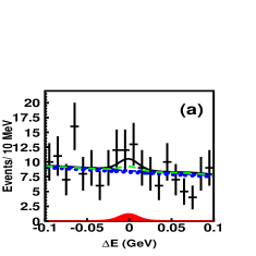
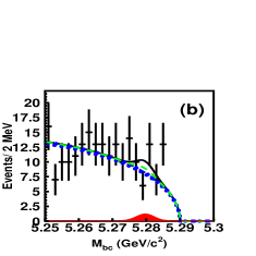
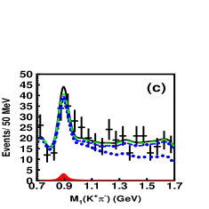
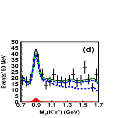
Figure 1: Projections of the four-dimensional fit onto (a) $\Delta E$, (b) $M_{\mathrm{bc}}$, (c) $M(K^{+}\pi^{-})$, and (d) $M(K^{-}\pi^{+})$ for candidates satisfying (except for the variable plotted) $\Delta E\in[-0.045,\ 0.045]\ \mathrm{GeV}$, $M_{\mathrm{bc}}\in[5.27,\ 5.29]\ \mathrm{GeV}/c^{2}$, and $M_{1,2}(K\pi)\in[0.826,\ 0.966]\ \mathrm{GeV}/c^{2}$. The thick solid curve shows the overall fit result; the solid shaded region represents the $B^{0}\to K^{*0}\overline{K}{}^{*0}$ signal component; and the dotted, dot-dashed and dashed curves represent continuum background, $b\to c$ background, and charmless $B$ decay background, respectively.

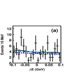
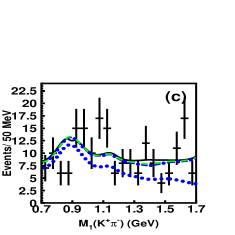
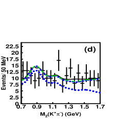
Figure 2: Same as for Fig. 1 but for the $B^{0}\to K^{*0}K^{*0}\to(K^{+}\pi^{-})(K^{+}\pi^{-})$ study: (a) $\Delta E$, (b) $M_{\mathrm{bc}}$, (c) $M_{1}(K^{+}\pi^{-})$, and (d) $M_{2}(K^{+}\pi^{-})$.

To check our reconstruction efficiencies, we measure the yields of control samples $B^{0}\to D^{-}\pi^{+}\to(K^{+}K^{-}\pi^{-})\pi^{+}$ and $B^{0}\to\overline{D}{}^{0}K^{*0}\to(K^{+}\pi^{-})(K^{+}\pi^{-})$. These modes have a similar topology to the signal modes and are selected using the same selection criteria except that, instead of $D$ vetos, we require $|M(KK\pi)-m_{D^{\pm}}|<13\ \mathrm{MeV}/c^{2}$, $|M(K\pi)-m_{D^{0}}|<13\ \mathrm{MeV}/c^{2}$, and $826~{}\mathrm{MeV}/c^{2}<M(K\pi)<966~{}\mathrm{MeV}/c^{2}$. The efficiencies are 19% for $B^{0}\to D^{-}\pi^{+}$ and 11% for $B^{0}\to\overline{D}{}^{0}K^{*0}$. The difference in signal yields between the measured and expected values are $(5.8\pm 5.8)$% and $(5.6\pm 27.8)$% for $B^{0}\to D^{-}\pi^{+}$ and $B^{0}\to\overline{D}{}^{0}K^{*0}$, respectively. These differences are consistent with zero.

The systematic errors (in units of events) are summarized in Tables 2 and 3. For systematic uncertainties due to fixed yields, e.g., that of charmless $B$ background, we vary the yields by their uncertainties ($\pm 1\sigma$). For the systematic uncertainties due to $B^{0}\to K_{2}^{*}(1430)X$ decays, including $B^{0}\to K_{2}^{*}(1430)\overline{K}{}_{2}^{*}(1430)$, $B^{0}\to K_{2}^{*}(1430)\overline{K}{}_{0}^{*}(1430)$, $B^{0}\to K_{2}^{*}(1430)\overline{K}{}^{*0}$, and $B^{0}\to K_{2}^{*}(1430)K\pi$, we float their yields in the four-dimensional ML fit; the differences between these results and the nominal fit values are taken as systematic errors. Systematic uncertainties for the $\Delta E$-$M_{\rm bc}$ PDFs are estimated by varying the signal peak positions and resolutions by $\pm 1\sigma$ and repeating the fits. Systematic uncertainties for the $M_{1}$-$M_{2}$ PDFs are estimated in a similar way; we vary the mean and width of $K^{*0}$ and $K_{0}^{*}(1430)$ mass shapes according to the uncertainties in the world average values PDGroup . A systematic error for the longitudinal polarization fraction is obtained by changing the fraction from the nominal value $f_{\mathrm{L}}\!=\!1$ to the lowest possible value $f_{\mathrm{L}}\!=\!0$ when evaluating the reconstruction efficiency. According to MC simulation, the signal SCF fractions are 13.4% for (longitudinally polarized) $B^{0}\to K^{*0}\overline{K}{}^{*0}$, 7.9% for $B^{0}\to K^{*0}K\pi$, 6.7% for $B^{0}\to K_{0}^{*}(1430)\overline{K}{}_{0}^{*}(1430)$, 6.7% for $B^{0}\to K_{0}^{*}(1430)\overline{K}{}^{*0}$, 7.6% for $B^{0}\to K_{0}^{*}(1430)K\pi$, and 9.2% for nonresonant $B^{0}\to KK\pi\pi$. We estimate a systematic uncertainty due to these fractions by varying them by $\pm 50\%$.

A high-statistics MC study indicates that there are small fit biases; these are listed in Table 1. We find that fit biases occur due to the correlations between the two sets of variables ($\Delta E$, $M_{\rm bc}$) and ($M_{1}$, $M_{2}$), which are not taken into account in our fit. We correct the fitted yields for these biases. To take into account possible differences between MC simulation and data, we take both the magnitude of the bias corrections and the uncertainty in the corrections as systematic errors. The systematic errors for the efficiency arise from the tracking efficiency, PID, and the $\mathcal{R}$ requirement. The systematic error on the track-finding efficiency is estimated to be 1.2% per track using partially reconstructed $D^{*}$ events. The systematic error due to the PID is 1.0% per track as estimated using an inclusive $D^{*}$ control sample. The systematic error for the $\mathcal{R}$ requirement is determined from the efficiency difference between data and MC samples of $B^{0}\to D^{-}(K^{+}\pi^{-}\pi^{-})\pi^{+}$ decays.

Table 2: Summary of systematic errors (in units of events) for decay modes with a final state $K^{+}\pi^{-}K^{-}\pi^{+}$. The parameters $N_{B^{0}\to K_{2}^{*}(1430)X}$ and $N_{b\to u,d,s}$ (the other known charmless $B$ decays) correspond to branching fraction uncertainties for these charmless $B$ decays. Values for $f_{\mathrm{L}}$ and $f_{\mathrm{SCF}}$ are the uncertainties for longitudinal polarization and self-cross-feed, respectively.

Source	$K^{*0}\overline{K}{}^{*0}$	$K^{*0}K^{-}\pi^{+}$	$K_{0}^{*}(1430)\overline{K}{}_{0}^{*}(1430)$	$K_{0}^{*}(1430)\overline{K}{}^{*0}$	$K_{0}^{*}(1430)K^{-}\pi^{+}$	Nonresonant $K^{+}\pi^{-}K^{-}\pi^{+}$
Fitting PDF	$\pm 1.8$	$\pm 40.3$	$\pm 55.6$	$\pm 37.7$	$\pm 158.0$	$\pm 102.4$
$N_{B^{0}\to K_{2}^{*}(1430)X}$	$+1.1$	$+10.2$	$-7.1$	$-20.4$	$-52.8$	$-10.5$
$N_{b\to u,d,s}$	$\pm 0.0$	$\pm 0.1$	$\pm 0.2$	$\pm 0.1$	$\pm 0.7$	$\pm 1.0$
$f_{\mathrm{L}}$	$-0.1$	—	—	—	—	—
$f_{\mathrm{SCF}}$	$\pm 0.7$	$\pm 1.4$	$\pm 5.6$	$\pm 2.2$	$\pm 17.2$	$\pm 14.6$
Fit Bias	${}^{+1.5}_{-0.7}$	${}^{+2.9}_{-5.4}$	$\pm 5.1$	${}^{+13.3}_{-2.3}$	${}^{+8.9}_{-14.7}$	${}^{+7.3}_{-10.8}$
Tracking	$\pm 0.4$	$\pm 0.8$	$\pm 3.5$	$\pm 0.9$	$\pm 9.6$	$\pm 6.8$
PID	$\pm 0.4$	$\pm 0.7$	$\pm 2.9$	$\pm 0.7$	$\pm 8.2$	$\pm 6.0$
$\mathcal{R}$ requirement	$\pm 0.2$	$\pm 0.4$	$\pm 1.6$	$\pm 0.4$	$\pm 4.5$	$\pm 3.2$
$N_{B\overline{B}}$	$\pm 0.1$	$\pm 0.3$	$\pm 1.1$	$\pm 0.3$	$\pm 3.1$	$\pm 2.2$
Sum	${}^{+2.8}_{-2.1}$	${}^{+41.7}_{-40.7}$	${}^{+56.3}_{-56.8}$	${}^{+40.0}_{-43.0}$	${}^{+159.7}_{-168.6}$	${}^{+104.1}_{-104.9}$

Table 3: Same as for Table 2 but for decay modes with a final state $K^{+}\pi^{-}K^{+}\pi^{-}$.

Source	$K^{*0}K^{*0}$	$K^{*0}K^{+}\pi^{-}$	$K_{0}^{*}(1430)K_{0}^{*}(1430)$	$K_{0}^{*}(1430)K^{*0}$	Nonresonant $K^{+}\pi^{-}K^{+}\pi^{-}$
Fitting PDF	$\pm 2.4$	$\pm 40.0$	$\pm 20.7$	$\pm 22.5$	$\pm 30.5$
$N_{B^{0}\to K_{2}^{*}(1430)X,K_{0}^{*}(1430)K\pi}$	$-0.3$	$+16.8$	$+85.1$	$-20.2$	$-96.8$
$N_{b\to u,d,s}$	$\pm 0.0$	$\pm 0.4$	$\pm 0.1$	$\pm 0.3$	$\pm 0.3$
$f_{\mathrm{L}}$	$-0.7$	—	—	—	—
$f_{\mathrm{SCF}}$	$\pm 0.1$	$\pm 0.2$	$\pm 0.8$	$\pm 0.5$	$\pm 0.2$
Fit Bias	${}^{+0.5}_{-1.0}$	$\pm 2.7$	${}^{+1.3}_{-3.4}$	${}^{+8.2}_{-1.6}$	${}^{+7.7}_{-2.2}$
Tracking	$\pm 0.2$	$\pm 0.0$	$\pm 1.2$	$\pm 0.4$	$\pm 0.5$
PID	$\pm 0.2$	$\pm 0.0$	$\pm 1.0$	$\pm 0.3$	$\pm 0.4$
$\mathcal{R}$ requirement	$\pm 0.1$	$\pm 0.0$	$\pm 0.6$	$\pm 0.2$	$\pm 0.2$
$N_{B\overline{B}}$	$\pm 0.1$	$\pm 0.0$	$\pm 0.4$	$\pm 0.1$	$\pm 0.2$
Sum	${}^{+2.5}_{-2.7}$	${}^{+43.5}_{-40.1}$	${}^{+87.7}_{-21.1}$	${}^{+23.9}_{-30.3}$	${}^{+31.4}_{-101.5}$

In summary, we have used a data sample corresponding to $657\times 10^{6}$ $B\overline{B}$ pairs to search for $B^{0}\to K^{*0}\overline{K}{}^{*0}$, $B^{0}\to K^{*0}K^{*0}$, and other charmless decay modes with a $K^{+}\pi^{-}K^{\mp}\pi^{\pm}$ final state. We do not find significant signals for any of these modes. Our measured branching fraction for $B^{0}\to K^{*0}\overline{K}{}^{*0}$ is $(0.26^{+0.33+0.10}_{-0.29-0.07})\times 10^{-6}$, which is lower than that obtained by BaBar aaubert by 2.2$\sigma$. Our 90% C.L. upper limits are $0.8\times 10^{-6}$ for $\mathcal{B}(B^{0}\to K^{*0}\overline{K}{}^{*0})$ and $0.2\times 10^{-6}$ for $\mathcal{B}(B^{0}\to K^{*0}K^{*0})$; those for other decay modes are listed in Table 1.

We thank the KEKB group for excellent operation of the accelerator, the KEK cryogenics group for efficient solenoid operations, and the KEK computer group and the NII for valuable computing and SINET3 network support. We acknowledge support from MEXT, JSPS and Nagoya’s TLPRC (Japan); ARC and DIISR (Australia); NSFC (China); MSMT (Czechia); DST (India); MEST, NRF, NSDC of KISTI (Korea); MNiSW (Poland); MES and RFAAE (Russia); ARRS (Slovenia); SNSF (Switzerland); NSC and MOE (Taiwan); and DOE (USA).

References

(1)
Charge-conjugate modes are implicitly included
throughout this paper unless noted otherwise.
(2)A. Ali et al., Z. Phys. C 1, 269 (1979);
M. Suzuki, Phys. Rev. D 66, 054018 (2002).
(3)C.H. Chen, Y.Y. Keum, and H-n. Li, Phys. Rev. D 66,
054013 (2002).
(4)K.-F. Chen et al. (Belle Collaboration), Phys. Rev.
Lett. 94, 221804 (2005); B. Aubert (BaBar Collaboration), Phys. Rev.
Lett. 98 051801 (2007).
(5)A. Kagan, Phys. Lett. B 601, 151 (2004);
C. Bauer et al., Phys. Rev. D 70, 054015 (2004);
P. Colangelo et al., Phys. Lett. B 597, 291 (2004);
M. Ladisa et al., Phys. Rev. D 70, 114025 (2004);
H.-n. Li and S. Mishima, Phys. Rev. D 71, 054025 (2005);
M. Beneke et al., Phys. Rev. Lett. 96, 141801 (2006).
(6)H-n. Li, Phys. Lett. B 622, 63 (2005).
(7)A. Datta et al., Phys. Rev. D 76, 034051 (2007).
(8)D. Atwood and A. Soni, Phys. Rev. D 65, 073018 (2002);
S. Descotes-Genon, J. Matias and J. Virto, Phys. Rev. D 76, 074005 (2007).
(9)W. Zou and Z. Xiao, Phys. Rev. D 72, 094026 (2005);
M. Beneke, J. Rohrer, and D. Yang, Nucl. Phys. B774, 64 (2007).
H.-Y. Cheng and K.-C. Yang, Phys. Rev. D 78, 094001 (2008).
(10)D. Pirjol and J. Zupan, arXiv:0908.3150 [hep-ph].
(11)B. Aubert (BaBar Collaboration), Phys. Rev. Lett. 100,
081801 (2008).
(12)A. Abashian et al. (Belle Collaboration), Nucl. Instrum.
and Methods Phys. Res. Sect. A 479, 117 (2002).
(13)Z. Natkaniec et al. (Belle SVD2 Group), Nucl. Instrum.
and Methods Phys. Res. Sect. A 560, 1 (2006).
(14)S. Kurokawa and E. Kikutani, Nucl. Instrum. and Methods Phys.
Res. Sect. A 499, 1 (2003), and other papers included in this volume.
(15)D. J. Lange, Nucl. Instrum. Methods Phys. Res., Sect. A
462, 152 (2001).
(16)E. Barberio and Z. Wa̧s, Comput. Phys. Commun. 79, 291
(1994); P. Golonka and Z. Wa̧s, Eur. Phys. J. C 45, 97-107 (2006).
(17)R. Brun et al., GEANT 3.21, CERN Report DD/EE/84-1,
1984.
(19)G. C. Fox and S. Wolfram, Phys. Rev. Lett. 41, 1581 (1978).
The modified moments used in this paper are described in S. H. Lee et al.
(Belle Collaboration), Phys. Rev. Lett. 91, 261801 (2003).
(20)H. Kakuno et al., Nucl. Instrum. and
Methods Phys. Res. Sect. A 533, 516 (2004).
(21)H. Albrecht et al. (ARGUS Collaboration), Phys. Lett. B
241, 278 (1990).
(22)
C. Amsler et al. (Particle Data Group), Phys. Lett. B 667, 1 (2008).
(23)E. Barberio et al. (Heavy Flavor Averaging Group),
arXiv:0704.3575 [hep-ex].