Noise Properties of the Planck-LFI Receivers

Abstract

Aims. The Planck Low Frequency Instrument (LFI) radiometers have been tested extensively during several dedicated campaigns. The present paper reports the principal noise properties of the LFI radiometers.

Methods. A brief description of the LFI radiometers is given along with details of the test campaigns relevant to determination of noise properties.

Results. Current estimates of flight sensitivities, $1/f$ parameters, and noise effective bandwidths are presented.

Conclusions. The LFI receivers exhibit exceptional $1/f$ noise, and their white noise performance is sufficient for the science goals of Planck.

1 Introduction

The Low Frequency Instrument (LFI), installed on board the European Space Agency’s Planck satellite, is designed to measure temperature and polarization anisotropies of the cosmic microwave background (CMB) in three frequency bands from 30 to 70 GHz. The core of the Planck-LFI is a compact Radiometer Array Assembly (RAA) of 22 pseudo correlation radiometers, with cryogenic low-noise microwave amplifiers, which are coupled to the 1.5 meter Planck telescope by an array of 11 conical dual profiled corrugated feed horns. Design, construction and testing of the LFI are extensively described in a set of accompanying papers: Mandolesi (mandolesi09 (2009)), Bersanelli (bersanelli09 (2009)), Mennella (2009a ), Villa (villa09 (2009)), Sandri (sandri09 (2009)), Leahy (leahy09 (2009)). This work reports the noise performance of the Planck-LFI receivers measured in ground tests, and expected in-flight sensitivity.

In Section 2, we present a brief overview of the LFI receivers and their data acquisition system. In Section 3, we outline the noise properties being investigated. In Section 4, we describe the test campaigns and the main results obtained from them. In Section 5, we provide a summary and discussion of the LFI noise performance. In Section 6, we present the conclusion of this work.

2 Overview of the LFI receivers and data acquisition

A key objective of the Planck-LFI radiometer architecture is minimizing $1/f$ noise. Excess $1/f$ noise would degrade the radiometer’s sensitivity, increase the uncertainty in the measured angular power spectrum at low-$\ell$, and add a source of systematic errors that would propagate in a non-trivial way through the Planck-LFI scientific products (e.g. Maino maino02 (2002)).

Planck will observe the sky by continuously scanning nearly great circles on the celestial sphere with a one minute period, and periodically (approximately 50 minutes) shifting the spin axis to remain anti-sun throughout the year.

Each of the 11 LFI feed horns couples radiation from the Planck’s optics through a Receiver Chain Assembly (RCA), that consists of an actively-cooled 20 K Front-End Module (FEM) connected via waveguides to a 300 K Back-End Module (BEM), which is followed by the Data Acquisition Electronics (DAE), and Radiometer Electronics Box Assembly (REBA).

An Orthomode Transducer (OMT) separates the radiation that enters the RCA FEM into two orthogonally polarized components, and transmits each component to a pseudo correlation radiometer. A $180^{\circ}$ hybrid coupler combines the sky signal with the signal from a cooled (approximately 4 K) reference load viewed with a small feed horn. The two outputs of the hybrid are then amplified by cryogenic low-noise High Electron Mobility Transistor (HEMT) amplifiers and each passing through a 180 degree phase switch. One of the phase switches is modulated at 4096 Hz whilst the other remains unswitched. The two resulting signals run into a second 180^∘ hybrid coupler. The FEM RF signals are then transmitted via waveguides to the Back End Module (BEM), where they are further amplified, filtered, and detected by square-law diodes (Aja 2005a , 2005b , Artal artal09 (2009)). The BEMs include preamplifiers the detector diodes to raise the signal level before input to the Data Acquisition Electronics (DAE). The outputs of the detectors form two independent streams of data alternating between sky and reference at 4096 Hz for each radiometer, or four independent streams per RCA. A general analytical description of the Planck-LFI radiometers is given by Seiffert (seiffert02 (2002)), and Mennella (mennella03 (2003)).

The BEM outputs pass to the DAE, where a programmable offset and gain are applied to optimize the dynamic range. The signals are then integrated in an ideal integrator circuit, and converted from analog to digital signals. The digitized output is downsampled, mixed, re-digitized, compressed, and transmitted to telemetry by software in the REBA (Maris maris09 (2009)). The difference between sky and reference is not calculated at this stage. It is calculated on the ground, after data have been decompressed, demixed and time streams are reconstructed (Zacchei zacchei09 (2009)). With only the data acquired from a given diode we create sky-only, and reference-only time streams, allowing us to compute the uncalibrated differenced time stream $V_{\mathrm{diff}}$ as

$$V_{\mathrm{diff}}=V_{\mathrm{sky}}-rV_{\mathrm{ref}},$$ (1)

where $V_{\mathrm{sky}}$ is the uncalibrated sky-only time stream, $V_{\mathrm{ref}}$ is the uncalibrated reference-only time stream, and $r$ is a gain modulation factor that brings the difference as close as possible to zero, simultaneously minimizing $1/f$ and equalizing the white noise contributions of sky and reference data samples. A value of $r$ equal to the ratio of the means of the sky and reference time streams achieves this goal (e.g. Mennella mennella03 (2003); see also discussion in Section 5.1.1). Finally, the calibrated differenced time stream $T_{\mathrm{diff}}$ is then computed as

$$T_{\mathrm{diff}}=GV_{\mathrm{diff}},$$ (2)

where $G$ is the photometric calibration, valid in the linear response range of the instrument, which converts the output voltage into Rayleigh-Jeans temperature units. Figure 1 displays a schematic of one LFI radiometer and its data acquisition system.

The main advantages of the LFI radiometer design are: (i) its sensitivity does not depend (to first order) on the absolute level of the reference signal, even in the case of a slight imbalance of the radiometer’s components; (ii) with the proper gain modulation factor, the $1/f$ noise in the radiometer time streams depends mostly on the noise temperature fluctuations of the FEM amplifiers; (iii) the $1/f$ fluctuations from gain fluctuation in the BEM amplifiers are effectively removed by the fast switching between sky and reference signals.

It is worth noting explicitly that the noise performance of LFI, in particular the $1/f$ noise, is dependent to some extent on every element in the receiver chain, from the emissivity and temperature stability of the reflectors, to the frequency dependent match and loss of the passive front end components, the stability and match of the reference horns and loads, the thermal stability of the back ends, as well as the electrical and thermal stability of the downstream electronics. First order fluctuations induced after the FEM are very effectively removed by the differencing of sky and reference time streams for each diode, switching at 4 KHz. Second order fluctuations, and those induced by temperature changes in the front end are not removed by the switching.

As a unique feature of LFI, the 4K reference loads, as well as the reference horns used to view them, have undergone careful design and testing (Valenziano, 2009). The horn/load coupling return loss was measured via network analyzer, and all horn/load combinatgions met the requirement of -20 dB integratedas measured by the Return Loss reference horn-loads ( using SNA on optical bench) The requirement was to be better then -20 dB

All the reference loads satisfy this requirement; performance change with the frequency , since loads and horns have been projected different depending on the frequency ( actually waveguides dimensions do not scale in size with frequency , as well as the gaps reference horn - reference load, being constant while Lambda is changing with channels) . The req. is given as integrated mismatching along the full bandwidth , hence the return loss level for particular frequencies can also be higher than the requirement . The reference horn insertion loss was roughly measured by shortening the horn and measuring S11: result is a worst case and is in all the cases better than 0.15 dB . The spillover, accounting for the internal straylight , is lower than -40 dB ; external sky radiation, passing through the main frame , is further dumped and is found lower than -60 dB . In both cases spillover is just simulated and not calculated.

In this paper we analyze results of tests with representative conditions achievable in the instrument test campaigns. In particular, we do not describe data where the flight cooling chains were employed. The test campaigns included explicit tests for susceptibility to the various effects noted above but the actual fluctuations induced by the cooling chains were not measured until the satellite integration tests (not covered by this work). The impact of the sorption cooler and 4 K cooler on the performance of LFI is non trivial, but has been investigated through extensive simulations and measurements of the cooling chain. There is a specification for fluctuations of the 4 K load of 10 $\mu\mathrm{K}/\sqrt{\mathrm{Hz}}$. In general, $1/f$ is dominated by the receiver characteristics, not random thermal fluctuations in the loads or passive optical elements. We do anticipate measurable signals in LFI due to the cycling of the sorption cooler. This is regular and predictable, and couples to the radiometer outputs through the channels mentioned above. These issues are explored most comprehensively in Terenzi 2009a , and 2009b . All of these effects will be studied exhaustively both using the satellite test campaign, and of course the flight data.

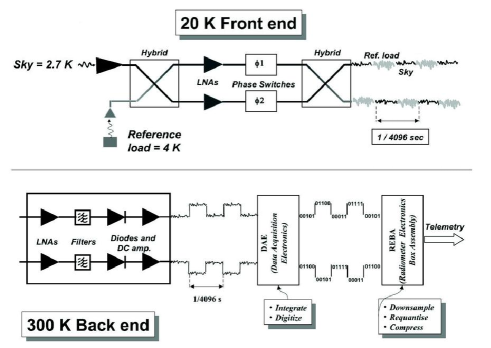
Figure 1: Schematic of one LFI radiometer and its data acquisition system. The outputs of the radiometer form two independent streams of data alternating between the signals from the sky and from a stable internal cryogenic reference load. The radiometer architecture is designed to efficiently minimize the $1/f$ noise on the post detection differenced time stream defined in Equation 1. This figure is adapted from Seiffert (seiffert02 (2002)).

3 Noise model

Several tests were performed on the RCA and RAA instruments to investigate and characterize the noise of the LFI radiometers.

We parameterize the noise power spectral density $P(f)$ as

$$P(f)\sim\sigma^{2}\left[1+\left(\frac{f}{f_{\mathrm{k}}}\right)^{\alpha}\right],$$ (3)

where $\sigma$ characterizes the white noise component, the knee frequency $f_{\mathrm{k}}$ denotes the frequency where white noise and $1/f$ contribute equally to the total noise, and $\alpha$ characterizes the slope of the power spectrum for frequencies $f<f_{\mathrm{k}}$.

We use the radiometer equation to evaluate how well the white noise level corresponds to expectation based on the system temperature, which is given as

$$\sigma_{T}=K\left(\frac{T_{\mathrm{noise}}+T_{\mathrm{target}}}{\sqrt{\beta_{\mathrm{eff}}\tau}}\right),$$ (4)

where $\sigma_{T}$ is the root-mean-square noise, $T_{\mathrm{noise}}$ is the system noise temperature, $T_{\mathrm{target}}$ is the antenna temperature of the target being observed, $\beta_{\mathrm{eff}}$ is the noise effective bandwidth, $\tau$ is the integration time, and $K$ is a constant of order unity which depend on the receiver architecture (see Appendix A for details), e.g. Kraus (kraus86 (1986)).

In addition to tracking the white noise level, knee frequency and slope, we use the noise effective bandwidth $\beta_{\mathrm{eff}}$ as a figure of merit for checking white noise consistency. The noise effective bandwidth can be interpreted as the width of an ideal rectangular RF band-pass filter which would produce the same noise power as the noise measured from the real instrument. In an ideal radiometer (i.e. when input target temperature is proportional to output voltage signal), it can be estimated from the data as

$$\beta_{\mathrm{eff}}=\left(\frac{KV_{\mathrm{DC}}}{\sigma_{\mathrm{V}}}\right)^{2},$$ (5)

where $V_{\mathrm{DC}}$ is the uncalibrated offset when observing the target, and $\sigma_{\mathrm{V}}$ is the uncalibrated white noise. The noise effective bandwidth is independent of gain, independent of system and target temperatures, specifically sensitive to voltage offsets, and external noise such as electromagnetic interference (EMI). This is why $\beta_{\mathrm{eff}}$ is a good figure of merit for checking noise consistency. It should be noted here that because the RAA test campaign operated the 30 and 44 GHz radiometers in a slightly compressed state, a minor modification to Equation 5 is needed for these receivers, and $\beta_{\mathrm{eff}}$ should be estimated as

$$\beta_{\mathrm{eff}}=\left(\frac{KV_{\mathrm{DC}}}{\sigma_{\mathrm{V}}}\right)^{2}\times[1+bG(T_{\mathrm{noise}}+T_{\mathrm{target}})]^{-2},$$ (6)

where $T_{\mathrm{noise}}$ is the system noise temperature, $T_{\mathrm{target}}$ is an input temperature, and $b$ is a non linearity parameter. This is discussed in detail in Mennella (2009a , 2009b ).

Investigation of noise properties of LFI during the several test campaigns characterized the instrument performance, but also served to uncover subtle systematic effects from instrument anomalies. In all cases the analysis allowed us to track down and solve the problems. One example was the occurrence of ‘telegraph’ or ‘popcorn’ noise, which was traced to an oscillating BEM which was eventually replaced. During another campaign, excessive $1/f$ noise in a 44 GHz radiometer was traced to a damaged phase switch on a 70 GHz radiometer which shares the same power supply. This was solved by changing the operating mode of the 70 GHz phase switch. During test campaigns in Finland and Laben several frequency spikes were seen in the power spectra, which were finally proven to be from the ground electronics, and completely absent in the satellite level tests. An exception is the set of spikes caused by the housekeeping data acquisition, which is described in detail in section 5.1.2. Ultimately, the best description of the LFI noise properties is the very simple model given by Equation 3.

4 Test campaign

The LFI test campaign included breadboard, qualification model, and flight model tests. Testing was performed at amplifier level, RCA level, and RAA level (Tanskanen tanskanen00 (2000), Kangaslahti kangaslahti01 (2001), Sjöman sjoman03 (2003), Laaninen laaninen06 (2006), Terenzi 2009a , Davis davis09 (2009), Artal artal09 (2009), Villa villa09 (2009), Varis varis09 (2009)). This work focuses on the flight model tests at RCA and RAA level. Noise properties considered here were measured after an extensive tuning procedure (Cuttaia 2009a ), which involved optimizing the cryogenic amplifier biases for system noise and bandwidth, matching phase switch response, and tuning for overall ‘isolation’ between the two output states which measure sky and reference load temperatures.

4.1 RCA Campaigns

Basic parameters for the LFI receivers were measured in detail during the RCA test campaigns. These measurements and results are discussed in Villa villa09 (2009) and references above. In addition we emphasize the following relevant points about these data sets.

1. Direct swept source measurements of the bandwidths are generally consistent with noise estimated bandwidths (Zonca zonca09 (2009)).

2. Measured temperature calibrated white noise is generally consistent with the measured $T_{\mathrm{noise}}$ and Equation 4.

3. For 30 and 44 GHz RCAs, the measured $1/f$ knees are well below the specification of 50 mHz, while for 70 GHz the sky load was not stable enough to measure this.

4. Gain compression was measured for all RCAs. All will be in the linear regime for flight operations.

5. 70 GHz RCAs are linear over all test conditions (RCA and RAA).

6. 30 and 44 GHz RCAs are compressed. Thus careful calibration of the compression curves were carried out to help predict performance for different target temperatures.

4.2 RAA Campaign

After RCA testing, the receivers were installed in the full array and retested as the RAA in the Thales Alenia Space Italia laboratories. In this test flight hardware (electronics, harnesses and computer) was used. This test campaign included tuning, interference tests, system temperature, and noise characterization among many other things. A single large sky load was used, with very good long term stability. This allowed more careful measurement of LFI’s very low $1/f$ noise. For detailed description of the test systems, including thermal, electrical, RF and mechanical design of the loads and chamber see Terenzi (2009b ), Morgante (morgante09 (2009)), and Cuttaia (2009b ).

Due to the size of the sky load and the design of the chamber, RAA sky and reference loads could not be cooled below about 18 K, and sky load time constants were many hours. This allowed complete system tests, $1/f$ measurements, crosstalk measurements, tuning etc, but provided some limitations with respect to noise parameters.

System temperature measurements from RCA tests were more reliable than from RAA tests, due to complications from gain compression, thermal gradients and limited temperature step sizes. The long time constants of the loads for RAA testing also limited the number of temperature steps to three, leaving the fits poorly constrained.

Temperature calibrated white noise levels were similarly affected by compression and temperature gradients (causing systematic errors in our estimates of the gain). Noise temperature and, ultimately, white noise sensitivity were also affected by the fact that the Focal Plane Unit (FPU) temperature was kept at about 26 K, instead of the 20 K as it is going to be the case during flight.

A campaign to analyze the thermal and RF properties of the full system has been carried out with some success, and is described in some of the references above. However, for our purposes in characterizing the LFI FM noise performance we prefer to take the best measurements from each of the test campaigns, in addition to providing evidence for consistency among tests wherever possible.

4.2.1 RAA results

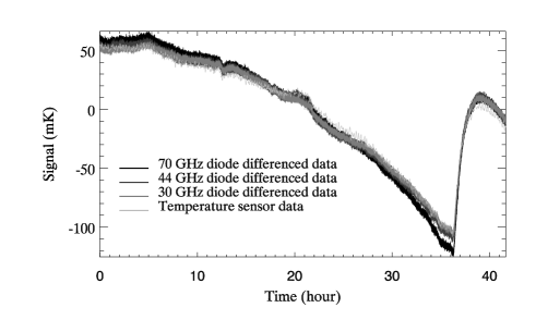
Figure 2: Comparison between scientific and thermal environment time streams from data in ST1_0002. The mean was removed from the temperature sensor. The radiometer’s differenced data follow the thermal environment behavior. The small differences between them are due to a temperature gradient in the microwave absorber. The long term offset changes due to a slow and continuous change in reference temperature ($\sim 0.7$ mK/hour), which reaches a minimum at 36h. This behavior was due to a small leak in one of the gaseous helium heat switches of the cryo chamber. Despite this drift, the test provided many hours of stable data that were useful for characterization of LFI RAA noise properties.

Our primary source for information on the $1/f$ performance of LFI RAA is a long ($44.3$ hours) data set acquired in near nominal thermal environment and nominal optimized biases for all channels. During its data acquisition, the physical temperatures of the microwave absorber and the reference load were kept at about 22 K and 19 K, respectively. The length of the data set allowed us to investigate stability of the noise parameters as well as different techniques and timescales for calculating the gain modulation factor. In addition we have very good statistics to look for systematic effects such as crosstalk and anomalous frequency spikes in the data. Data were acquired with sample rates of 32.5 Hz, 46.5 Hz, and 78.8 Hz, for 30 GHz, 44 GHz, and 70 GHz channels respectively. Figure 2 shows examples of differenced time streams from the long data set. For the purposes of noise analysis, the salient features of the RAA data sets include:

1. Noise effective bandwidths are consistent with RCA test campaign results including both white noise and swept source derived values.

2. $1/f$ knee measurements are within specification ($<50$ mHz).

3. White noise, system temperature and effective bandwidth are consistent with Equation 4.

4. The sky and reference load temperatures were not kept lower than 19 K, a deviation from flight conditions.

5. For these input conditions, some channels show some gain compression.

5 Summary and discussion

The principal results from the RAA campaign are summarized in Table 1. In Section 5.1, we discuss how these results were obtained.

5.1 Procedure

For each LFI diode, uncalibrated and calibrated differenced time streams were produced applying Equations 1 and 2 to the long data set mentioned in Section 4.2.1. A time stream containing $10^{5}$ seconds of calibrated differenced data were analyzed in $25$ individual $4000$ second sections, providing statistics for estimating the scatter in the noise parameters and a way to weight the parameter fits. For each data section, a Power Spectral Density (PSD) was computed. The PSD’s for all the sections for each diode were averaged and white noise, $1/f$ knee and slope estimated from a fit to Equation 3. Additionally, noise effective bandwidths were estimated from Equation 5 and, when needed, the results of the correction given by Equation 6 were included in the tabulated values of Table 1. The formal statistical uncertainties in the parameters are all approximately $1\%$. We should note that a single value of the gain modulation factor $r$ was used for the entire $10^{5}$ seconds for each diode, however, no significant change in parameters was found when $r$ was calculated for the individual sections. As an example, Figure 3 shows a comparison between data and model for one LFI diode radiometer.

5.1.1 Noise stability and crosstalk

These data sets display quite good stability of the noise parameters. As can be seen in Table 1, standard deviations for white noise and $1/f$ knee are typically less than $1\%$.

We have also tested a noise model with two independent $1/f$ components added to white noise. The idea behind this model is to try to separate intrinsic $1/f$ noise, which comes from the amplifiers, from $1/f$ noise coming from fluctuations in the temperature of the array or cold loads. For some data sets, the two $1/f$ component model gives a slightly better fit, but in general the single component model fits very well, particularly in the primary Planck data band (from the spin rate near 0.01 Hz to the Nyquist sampling rate).

The determination of the gain modulation factor $r$ provides another test for the robustness of the LFI receivers. The factor $r$ may be calculated over very long (month or more) timescales, or over times as short as a single satellite repointing (of order 1 hour), which is the baseline. We varied the timescale over which $r$ was calculated for the test data set from 1 to 30 hours, the maximum available. We find no significant change in white noise or $1/f$ performance. There is a clear increase in the $1/f$ noise when the $r$ factor is explicitly set wrong. Figure 4 shows an example of the dependence of $1/f$ performance as a function of variations in $r$.

The design of LFI is well optimized against crosstalk. Every detector diode has its own ADC, and the biases are independently controlled. We have attempted to find an intrinsic cross correlation among channels with no success. The long data set discussed here includes a small drift in the temperature of the load ($0.7$ mK/hour), which dominates any intrinsic cross correlation in the RCA outputs.

5.1.2 Frequency spikes

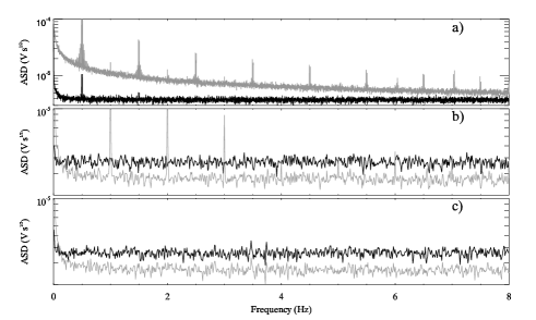
Figure 5: Comparison of frequency spikes for different configurations from a 44 GHz LFI receiver (diode $24s1$). ASDs from differenced data are displayed in black. ASDs from sky-only data are displayed in gray. Panel (a) shows data from the RAA test campaign. Note that the frequency spikes start at 0.5 Hz, and are greatly reduced by differencing. Panels (b) and (c) show data from the functionality test campaign at ambient temperature in Cannes, France. Here the spikes exactly cancel in the difference. Panel (c) shows data taken in Cannes with the housekeeping acquisition disabled, and clearly shows no spikes at all.

Some of the LFI receivers exhibit a small artifact, visible in the power spectra over long periods. The effect is noticeable as a set of extremely narrow spikes at 1 Hz and harmonics. These artifacts are nearly identical in sky and reference samples, and are (almost) completely removed by the LFI differencing scheme as can be seen in the top panel of Figure 5.

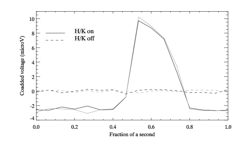
Figure 6: Here, one hour of sky-only data from a 44 GHz LFI receiver (diode $24s1$), acquired during the Cannes campaign, have been binned in time, synchronously with the housekeeping acquisition. We have removed offsets for every second of data for clarity. The disturbance due to the housekeeping acquisition is very evident from about $0.5$ to $0.75$ seconds. Once again we have included data with and without the housekeeping acquisition enabled.

Extensive testing and analysis has identified the spikes as a subtle disturbance on the science channels from the housekeeping data acquisition, which is also performed by the DAE (albeit with independent ADCs and electronics) at 1 Hz sampling. This causes the disturbance to be exactly synchronized with the science data, which makes it more visible and easier to remove. Figure 5 shows data from ambient temperature functional tests with and without the housekeeping data acquisition operational. These data come from tests done at the satellite integration level in Cannes, France in 2008. During these tests the LFI front end amplifiers were in a low gain state, making it easier to investigate subtle electronic interference such as these spikes. There are three significant things to notice here: the spikes only occur when the housekeeping acquisition is active; the spikes are exactly common mode for the balanced situation of the ambient tests; the spikes for the Cannes tests are 1 Hz and harmonics. The earlier test shown in the upper panel included spikes at harmonics of 0.5 Hz. This has been shown to be an artifact of the RAA test chamber: all subsequent tests, including fully integrated satellite tests done in Liege, Belgium in summer 2008 have shown the well understood 1 Hz spikes. Figure 6 demonstrates the way this disturbance is synchronized in time. These data were taken with very low thermal noise, to enhance the appearance of the disturbance. The data have been binned synchronously with the one second housekeeping sampling, and the disturbance due to the acquisition is very clear. This plot is for undifferenced data, the scientific data after difference show no significant disturbance. Despite the amelioration of the spikes by differencing, software tools have been developed to remove the disturbance from the limited number of channels showing it, and have been tested on the full Planck system tests carried out at the Centre Spatial de Liège (CSL), in Belgium, in July and August of 2008. Part of the commissioning phase of Planck will include careful on-orbit characterization of the spikes to further optimize the tools. Monte Carlo testing of the LFI analysis pipeline includes simulations and removal of these spikes.

5.2 Estimated flight sensitivity

The in-flight radiometer’s sensitivity was estimated from extrapolating white noise RAA measurements, obtained at $20$ K sky load temperature, to the expected calibrated sensitivity in flight conditions. The procedure considers a general radiometric output model, including non linearity, in which the LFI receiver voltage output $V_{\mathrm{out}}$ is provided by

$$V_{\mathrm{out}}=\frac{G(T_{\mathrm{noise}}+T_{\mathrm{target}})}{1+bG(T\mathrm{{}_{noise}}+T_{\mathrm{target}})},$$ (7)

where $G$ is the photometric calibration in the limit of linear response, $T_{\mathrm{noise}}$ is the system noise temperature, $T_{\mathrm{target}}$ is an input temperature, and $b$ is a non linearity parameter (Daywitt daywitt89 (1989)). These parameters were obtained from dedicated tests during the RAA campaign combined with compression test results from the RCA campaign. We extrapolate the uncalibrated white noise measured with a sky load temperature of $20$ K, to estimate calibrated white noise when $T_{\mathrm{target}}$ corresponds to the antenna temperature of the microwave sky. The extrapolation is dominated by the change of the sky load temperature, but the calculation includes a correction for system temperature with FPU temperature, as well as proper noise weighted averaging of the two detector diodes of each radiometer. The LFI sensitivity predictions are provided in Table 2.

6 Conclusion

The Planck-LFI noise has been extensively characterized during several cryogenic test campaigns. The receivers display exceptional $1/f$ noise performance and stability, and the estimated sensitivities are within twice the goal values. Careful examination of noise performance results from independent tests at various integration levels has allowed quantitative confirmation of the most important instrumental effects, including compression, noise effective bandwidth, gain modulation factor, and noise artifacts.

Table 1: Noise performance summary from RAA tests. For convenience, $T_{\mathrm{noise}}$ measurements from RCA tests (Villa villa09 (2009)) are also provided. Temperatures are quoted in Rayleigh-Jeans units.

$$\begin{array}[]{lcccccc}\hline\cr\vskip 3.0pt plus 1.0pt minus 1.0pt\cr Diode&\sigma_{T}^{20\mathrm{K}}(\mu\mathrm{K}\sqrt{\mathrm{s}})&f_{\mathrm{k}}(\mathrm{mHz})&\alpha&\beta_{\mathrm{eff}}(\mathrm{GHz})&\chi^{2}_{\nu}&T_{\mathrm{noise}}(\mathrm{K})\\ \vskip 3.0pt plus 1.0pt minus 1.0pt\cr\hline\cr\vskip 3.0pt plus 1.0pt minus 1.0pt\cr\underline{\mathbf{70GHz}}&&&&&&\\ 18m0&-\ (-)&-\ (-)&-\ (-)&-&-&36.0\\ 18m1&-\ (-)&-\ (-)&-\ (-)&-&-&36.1\\ 18s0&1124\ (0.02\%)&61\ (1\%)&-1.12\ (1\%)&11.8&1.40&33.9\\ 18s1&1072\ (0.02\%)&59\ (1\%)&-1.12\ (1\%)&15.0&1.40&35.1\\ 19m0&1214\ (0.02\%)&25\ (2\%)&-1.27\ (2\%)&10.1&1.26&33.1\\ 19m1&1165\ (0.02\%)&32\ (1\%)&-1.22\ (1\%)&10.4&1.27&31.5\\ 19s0&1113\ (0.02\%)&27\ (2\%)&-1.11\ (2\%)&10.7&1.29&32.2\\ 19s1&1109\ (0.02\%)&37\ (2\%)&-1.02\ (1\%)&12.1&1.28&33.6\\ 20m0&1094\ (0.02\%)&21\ (2\%)&-1.47\ (2\%)&11.6&1.29&35.2\\ 20m1&1138\ (0.02\%)&19\ (2\%)&-1.64\ (3\%)&10.5&1.32&34.2\\ 20s0&1195\ (0.02\%)&23\ (2\%)&-1.27\ (2\%)&10.6&1.31&36.9\\ 20s1&1145\ (0.02\%)&28\ (2\%)&-1.24\ (2\%)&11.7&1.31&35.0\\ 21m0&866\ (0.02\%)&28\ (2\%)&-1.48\ (2\%)&12.3&1.34&27.3\\ 21m1&891\ (0.02\%)&30\ (1\%)&-1.61\ (2\%)&12.8&1.35&28.4\\ 21s0&1193\ (0.02\%)&41\ (1\%)&-1.15\ (1\%)&12.2&1.30&34.4\\ 21s1&1279\ (0.02\%)&38\ (1\%)&-1.17\ (1\%)&10.8&1.29&36.4\\ 22m0&1029\ (0.02\%)&46\ (1\%)&-1.18\ (1\%)&12.2&1.29&30.9\\ 22m1&1048\ (0.02\%)&39\ (1\%)&-1.26\ (1\%)&11.5&1.28&30.3\\ 22s0&943\ (0.02\%)&41\ (1\%)&-1.19\ (1\%)&13.0&1.28&30.3\\ 22s1&1008\ (0.02\%)&76\ (1\%)&-1.01\ (1\%)&13.6&1.30&31.8\\ 23m0&1038\ (0.02\%)&30\ (2\%)&-1.11\ (2\%)&12.7&1.28&35.9\\ 23m1&964\ (0.02\%)&31\ (2\%)&-1.19\ (2\%)&14.3&1.27&34.1\\ 23s0&1137\ (0.02\%)&58\ (1\%)&-1.15\ (1\%)&13.8&1.26&33.9\\ 23s1&1116\ (0.02\%)&75\ (1\%)&-1.12\ (1\%)&13.5&1.28&31.1\\ \underline{\mathbf{44GHz}}&&&&&&\\ 24m0&-\ (-)&-\ (-)&-\ (-)&-&-&15.5\\ 24m1&-\ (-)&-\ (-)&-\ (-)&-&-&15.3\\ 24s0&1320\ (0.03\%)&39\ (1\%)&-1.06\ (1\%)&3.6&1.27&15.8\\ 24s1&1129\ (0.03\%)&46\ (1\%)&-1.11\ (1\%)&4.7&1.37&15.8\\ 25m0&1295\ (0.03\%)&31\ (2\%)&-1.07\ (1\%)&4.1&1.31&17.5\\ 25m1&1276\ (0.03\%)&31\ (2\%)&-1.03\ (1\%)&4.2&1.45&17.9\\ 25s0&1280\ (0.03\%)&21\ (2\%)&-1.10\ (2\%)&3.6&1.34&18.6\\ 25s1&1124\ (0.04\%)&30\ (3\%)&-1.00\ (2\%)&4.8&2.41&18.4\\ 26m0&1216\ (0.03\%)&61\ (1\%)&-1.01\ (1\%)&4.3&1.31&18.4\\ 26m1&1257\ (0.03\%)&61\ (1\%)&-1.01\ (1\%)&3.9&1.31&17.4\\ 26s0&1277\ (0.03\%)&61\ (1\%)&-1.05\ (1\%)&3.4&1.27&16.8\\ 26s1&1111\ (0.02\%)&-\ (-)&-\ (-)&4.8&-&16.5\\ \underline{\mathbf{30GHz}}&&&&&&\\ 27m0&942\ (0.03\%)&30\ (2\%)&-1.06\ (2\%)&4.7&1.30&12.1\\ 27m1&949\ (0.03\%)&30\ (2\%)&-1.13\ (2\%)&4.6&1.31&11.9\\ 27s0&907\ (0.03\%)&27\ (2\%)&-1.25\ (2\%)&5.3&1.28&13.0\\ 27s1&966\ (0.03\%)&26\ (2\%)&-1.13\ (2\%)&4.5&1.28&12.5\\ 28m0&1001\ (0.04\%)&37\ (2\%)&-0.94\ (1\%)&4.1&1.29&10.6\\ 28m1&1051\ (0.04\%)&31\ (2\%)&-0.93\ (2\%)&3.8&1.30&10.3\\ 28s0&917\ (0.03\%)&37\ (2\%)&-1.07\ (1\%)&4.7&1.28&9.9\\ 28s1&929\ (0.03\%)&39\ (2\%)&-1.06\ (1\%)&4.6&1.29&9.8\\ \vskip 3.0pt plus 1.0pt minus 1.0pt\cr\hline\cr\end{array}$$

The provided parameters are defined within the model given by Equation 3. The errors reported in parentheses are derived from the scatter in the power spectra of individual data sections (see Section 5.1). The LFI radiometers at 70 GHz are identified with RCA labels from 18 to 23. The radiometers at 44 GHz are designated with labels from 24 to 26. The radiometers at 30 GHz are labelled as 27 and 28. The letters $m$ and $s$, respectively, indicate if a given radiometer is connected to the main or side OMT. The indexes 0 and 1 identify one of the two radiometer’s diode. RCA 18$m$ and RCA 24$m$ were not operational during RAA testing, and were subsequently repaired. A wrong set of REBA compression parameters was applied to RCA 26$s$1 during the long integration test, and white noise only has been estimated from another (much shorter) data set. These channels were characterized during the final cryogenic test in July, 2008.

Table 2: Estimated flight sensitivity from noise measurements extrapolation (see Section 5.2). The sensitivity goals for individual radiometers at 30, 44 and 70 GHz were 170, 200, and 270 $\mu\mathrm{K}\sqrt{\mathrm{s}}$, respectively. Requirements to achieve the core scientific aims of LFI are considered to be a factor of two worse than these goals. Estimations are quoted in Rayleigh-Jeans units.

$$\begin{array}[]{lclc}\hline\cr\vskip 3.0pt plus 1.0pt minus 1.0pt\cr Radiometer&\sigma_{T}^{flight}(\mu\mathrm{K}\sqrt{\mathrm{s}})&Radiometer&\sigma_{T}^{flight}(\mu\mathrm{K}\sqrt{\mathrm{s}})\\ \vskip 3.0pt plus 1.0pt minus 1.0pt\cr\hline\cr\vskip 3.0pt plus 1.0pt minus 1.0pt\cr\mathbf{70GHz}&&\mathbf{44GHz}&\\ \overline{\underline{2\times\mathrm{goal}}}&\overline{\underline{\mathbf{540}}}&\overline{\underline{2\times\mathrm{goal}}}&\overline{\underline{\mathbf{400}}}\\ 18m&-&24m&-\\ 18s&468&24s&447\\ 19m&546&25m&501\\ 19s&522&25s&492\\ 20m&574&26m&398\\ 20s&593&26s&392\\ 21m&424&\overline{\underline{\mathrm{weighted\ mean}}}&\overline{\underline{\mathbf{439}}}\\ 21s&530&\mathbf{30GHz}&\\ 22m&454&\overline{\underline{2\times\mathrm{goal}}}&\overline{\underline{\mathbf{340}}}\\ 22s&463&27m&241\\ 23m&502&27s&288\\ 23s&635&28m&315\\ \overline{\underline{\mathrm{weighted\ mean}}}&\overline{\underline{\mathbf{508}}}&28s&251\\ &&\overline{\underline{\mathrm{weighted\ mean}}}&\overline{\underline{\mathbf{269}}}\\ \vskip 3.0pt plus 1.0pt minus 1.0pt\cr\hline\cr\end{array}$$

Figure 3: Example of a power spectral density and a fit provided by the model comparison using differenced data from a 70 GHz LFI diode radiometer (diode $22m1$, as given in Table 1), integrated on the RAA, and viewing a microwave absorber kept at 22 K. The dotted line shows white noise level. The dashed lines intersect each other at the $1/f$ knee frequency.

Figure 4: Example of the $1/f$ knee frequency $f_{\mathrm{k}}$ from differenced data as a function of the gain modulation factor $r$. This result was computed using a time stream containing 32 hours of data from a 70 GHz LFI receiver (diode $20m0$). The internal box delimits the region which is within the Planck specification for $1/f$ performance. In this case, we verify that $f_{\mathrm{k}}<50\mathrm{mHz}$ for up to $\pm 0.5\%$ variations of the optimal value of $r$.

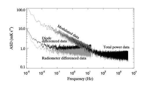
Figure 7: Example of an ASD comparison between different data acquisition modes. The effect of reducing $1/f$ noise due to switching is self evident. The effect of improving sensitivity by averaging data from two diodes is also evident. One can also note the change in the Nyquist frequency due to downsampling. Each acquisition mode sensitivity is consistent with what was expected from the most basic model (as described in Appendix A). This example shows the internal consistency presented by LFI among dedicated tests.

Appendix A Receiver sensitivity constant

In this work, we use Equation 4 to evaluate if, for any given LFI receiver, white noise corresponds to expectation. In that equation, the constant $K$ accounts for different radiometer topologies and differencing techniques. The purpose of this note is to clarify the relevant $K$ values for LFI, within the model given by Equation 4.

$K=1$.

This is the constant to be applied to Equation 4 when estimating sensitivity for a single LFI diode acquiring data in total power mode (i.e. an LFI diode receiver when not switching).

$K=\sqrt{2}$.

This is the constant to be applied to Equation 4 when estimating sensitivity for a single LFI diode acquiring data in modulated mode (i.e. an LFI diode receiver in switched condition). In this situation, the noise is higher because LFI spends only half of the available integration time looking to a given target. This is also the constant to be applied when estimating sensitivity for a single LFI radiometer (a single LFI radiometer provides data by averaging differenced data from two independent and complementary LFI diodes).

$K=2$.

This is the constant to be applied to Equation 4 when estimating sensitivity for differenced data from a single LFI diode. A degradation in the noise occurs because we use only half of the available integration time, and we also add the sky and reference noise in quadrature when performing the difference described by Equation 1.

Figure 7 shows a comparison between different LFI data acquisition modes that clearly illustrates the different LFI constant sensitivities.

Appendix B Amplitude spectral density normalization

The amplitude spectral density (ASD) is the square root of the power spectral density, and it is usually given in units of $\mathrm{K}/\sqrt{\mathrm{Hz}}$. The $1/\sqrt{\mathrm{Hz}}$ denotes that the value is per unit bandwidth, and is thus independent of the resolution bandwidth used to compute a result. Despite the apparent units, $\mathrm{K}/\sqrt{\mathrm{Hz}}$ and $\mathrm{K}\sqrt{\mathrm{s}}$ are not equivalent, and the purpose of this note is is to clarify the difference.

• $\mathrm{K}/\sqrt{\mathrm{Hz}}$ refers to an ‘integration bandwidth’ of 1 Hz, and assumes by convention a 6 dB/octave rolloff (obtainable from a 1 pole RC filter). This is the standard convention for ASD plots for historical reasons and comparisons with hardware FFT analyzers.

• $\mathrm{K}\sqrt{\mathrm{s}}$ refers to an integration time of 1 second. The effective integration time $\tau$ of a 1 Hz bandwidth is $0.5$ seconds. These units are easier for estimating sensitivity versus integration time.

Given these two definitions, we need to keep in mind the following unit conversion

$$\mathrm{K}/\sqrt{\mathrm{Hz}}=\sqrt{2}\times\mathrm{K}\sqrt{\mathrm{s}}.$$ (8)

For example, a time stream with white noise only, and samples at 1 second spacing with 1 K RMS, should produce an ASD with $1.414$ $\mathrm{K}/\sqrt{\mathrm{Hz}}$ everywhere. The assumption is that each sample in the time-ordered data was a $100\%$ duty cycle integration (i.e. 1 second long integration).

- (1) Aja, B., et al. 2005a, IEEE Trans. on Microwave Theory and Techniques, 53, 2050
- (2) Aja, B., et al. 2005b, IEEE Trans. on Aerospace and Electronic Systems, 41, 1415
- (3) Artal, E., et al. 2009, J-Inst, This issue
- (4) Bersanelli, M., et al. 2009, A&A, Submitted
- (5) Cuttaia, F., et al. 2009a, LFI radiometers: functionality and tuning, J-Inst, This issue
- (6) Cuttaia, F., et al. 2009b, High perfomance cryogenic blackbody calibrators: RAA, J-Inst, This issue
- (7) Davis, R., et al. 2009, J-Inst, This issue
- (8) Daywitt, W. C. 1989, Radiometer equation and analysis of systematic errors for the NIST automated radiometers, Technical Report, NIST/TN-1327
- (9) Kangaslahti, P., et al. 2001, Proc. IEEE MTT-S Int. Microwave Symposium, 1959
- (10) Kraus, J. D. 1986, Radio Astronomy, Powell, Ohio: Cygnus-Quasar Books
- (11) Laaninen, M., et al. 2006, Proc. 4th ESA Workshop on Millimetre Wave Technology and Applications, Espoo, 475
- (12) Leahy, P., et al. 2009, A&A, Submitted
- (13) Maino, D., et al. 2002, A&A, 387, 356
- (14) Maris, M., et al. 2009, J-Inst, This issue
- (15) Mandolesi, R., et al. 2009, A&A, Submitted
- (16) Mennella, A., et al. 2003, A&A, 410, 1089
- (17) Mennella, A., et al. 2009a, A&A, Submitted
- (18) Mennella, A., et al. 2009b, J-Inst, This issue
- (19) Morgante, G., et al. 2009, J-Inst, This issue
- (20) Sandri, M., et al. 2009, J-Inst, This issue
- (21) Seiffert, M., et al. 2002, A&A, 391, 1185
- (22) Sjöman, P., et al. 2003, Proc. 3rd ESA Workshop on Millimetre Wave Technology and Applications, Espoo, 75
- (23) Tanskanen, J. M., et al. 2000, IEEE Trans. Microwave Theory Tech., 48, 1283
- (24) Terenzi, L., et al. 2009a, High perfomance cryogenic blackbody calibrators: RCA, J-Inst, This issue
- (25) Terenzi, L., et al. 2009b, Cryogenic environment for testing the 30, 44 and 70 GHz Planck radiometers, J-Inst, This issue
- (26) Tomasi, M., et al. 2009, J-Inst, This issue
- (27) Varis, J., et al. 2009, J-Inst, This issue
- (28) Villa, F., et al. 2009, A&A, Submitted
- (29) Zacchei, A., et al. 2009, J-Inst, This issue
- (30) Zonca, A., et al. 2009, J-Inst, This issue