Ambiguities in recurrence-based complex network representations of time series

Abstract

Recently, different approaches have been proposed for studying basic properties of time series from a complex network perspective. In this work, the corresponding potentials and limitations of networks based on recurrences in phase space are investigated in some detail. We discuss the main requirements that permit a feasible system-theoretic interpretation of network topology in terms of dynamically invariant phase space properties. Possible artifacts induced by disregarding these requirements are pointed out and systematically studied. Finally, a rigorous interpretation of the clustering coefficient and the betweenness centrality in terms of invariant objects is proposed.

During the last decade, increasing interest has arisen in structural and dynamical properties of complex networks NetworkReviews . Particular efforts have been spent on reconstructing network topologies from experimental data, e.g., in ecology Montoya2006 , social systems Freeman1979 , neuroscience Zhou2006 , or atmospheric dynamics Donges2009 . The latter example yields a complex network representation of a continuous system, which suggests that applying a similar spatial discretization to the phase space of dynamical systems and using complex network methods as a novel tool for time series analysis could be feasible, too Zhang2006 ; Marwan2009 . For this purpose, different methods have been proposed (for a comparative review, see Donner2009 ) and successfully applied to real-world as well as model systems.

Many existing methods for transforming time series into complex network representations have in common that they define the connectivity of a complex network – similar to the spatio-temporal case – by the mutual proximity of different parts (e.g., individual states, state vectors, or cycles) of a single trajectory. In this work, we particularly consider recurrence networks, which are based on the concept of recurrences in phase space Eckmann1987 ; Marwan2007 and provide a generic way for analyzing phase space properties in terms of network topology Donner2009 ; Xu2008 ; Gao2009 ; Marwan2009 . Here, the basic idea is to interpret the recurrence matrix

$$R_{i,j}(\varepsilon)=\Theta(\varepsilon-\|\mathbf{x}_{i}-\mathbf{x}_{j}\|)$$ (1)

associated with a dynamical system’s trajectory, i.e., a binary matrix that encodes whether or not the phase space distance between two observed “states” $\mathbf{x}_{i}$ and $\mathbf{x}_{j}$ is smaller than a certain recurrence threshold $\varepsilon$, as the adjacency matrix of an undirected complex network. Since a single finite-time trajectory may however not necessarily represent the typical long-term behavior of the underlying system, the resulting network properties may depend – among others – on the length $N$ of the considered time series (i.e., the network size), the probability distribution of the data, embedding, sampling, etc. In the following, we present a critical discussion of the basic requirements for the application of recurrence networks and show that their insufficient application leads to pitfalls in the system-theoretic interpretation of complex network measures.

Threshold selection.

The crucial algorithmic parameter of recurrence-based time series analysis is $\varepsilon$. Several invariants of a dynamical system (e.g., the 2nd-order Rényi entropy $K_{2}$) can be estimated by taking its recurrence properties for $\varepsilon\to 0$ Marwan2007 , which suggests that for a feasible analysis of recurrence networks, a low $\varepsilon$ is preferable as well. This is supported by the analogy to complex networks based on spatially extended systems, where attention is usually restricted to the strongest links between individual vertices (i.e., observations from different spatial coordinates) for retrieving meaningful information about relevant aspects of the systems’ dynamics Zhou2006 ; Donges2009 . In contrast, a high edge density

$$\rho(\varepsilon)=\frac{2E(\varepsilon)}{N(N-1)}$$ (2)

(with $E(\varepsilon)$ being the total number of edges for a chosen $\varepsilon$) does not yield feasible information about the actually relevant structures, because these are hidden in a large set of mainly less important edges.

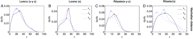
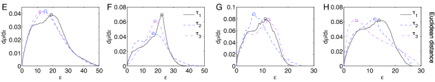
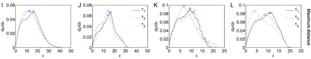
Figure 1: (Color online) Effects of different metrics and embeddings on the $\rho(\varepsilon)$ relationship, expressed in terms of the corresponding first derivative. (A,B,C,D): Manhattan distance; (E,F,G,H): Euclidean distance; (I,J,K,L): maximum distance. (A,E,I): Lorenz system $\left(\dot{x}=10(y-x),\ \dot{y}=x(28-z),\ \dot{z}=xy-\frac{8}{3}z\right)$ with original components at three different randomly chosen initial conditions. (B,F,J): Same Lorenz system embedded from the $x$ component with embedding delays $\tau_{1}=5,\tau_{2}=15$, and $\tau_{3}=20$. (C,G,K): same as (A,E,I) for the Rössler system $\left(\dot{x}=-y-z,\ \dot{y}=x+0.2y,\ \dot{z}=z(x-5.7)\right)$. (D,H,L): same as (B,F,J) for the Rössler system with $\tau_{1}=10,\tau_{2}=15$ and $\tau_{3}=20$. Circles indicate the respective maxima. In all cases, time series of $N=1,000$ points with a sampling time of $\Delta t=0.05$ have been used, obtained with a 4th-order Runge-Kutta integrator with fixed step width $h=0.01$. The values of $\tau_{2}$ are guided by the first zeros of the corresponding auto-correlation functions.

As a consequence, only those states should be connected in a recurrence network that are closely neighbored in phase space, leading to rather sparse networks. Following a corresponding rule of thumb recently confirmed for recurrence quantification analysis Schinkel2008 , we suggest choosing $\varepsilon$ as corresponding to an edge density $\rho\lesssim 0.05$ Marwan2009 ; Donner2009 , which yields neighborhoods covering appropriately small regions of phase space. Note that since many topological features of recurrence networks are closely related to the local phase space properties of the underlying attractor Donner2009 , the corresponding information is best preserved for such low $\varepsilon$ unless the presence of noise requires higher $\varepsilon$ Schinkel2008 .

Recently, a heuristic criterion has been proposed by Gao and Jin, which selects $\varepsilon$ as the (supposedly unique) turning point $\varepsilon_{crit}$ in the $\rho(\varepsilon)$ relationship of certain dynamical systems Gao2009 , formally reading

$$\left.\frac{d\rho}{d\varepsilon}\right|_{\varepsilon=\varepsilon_{crit}}=\max!,\quad\left.\frac{d^{2}\rho}{d\varepsilon^{2}}\right|_{\varepsilon=\varepsilon_{crit}}=0.$$ (3)

In contrast to our above considerations, for different realizations of the Lorenz system, this turning point criterion yields link densities of $\rho_{crit}=\rho(\varepsilon=\varepsilon_{crit})\sim 0.15\dots 0.3$ Gao2009 , implying that considerably large regions of the attractor are covered by the corresponding neighborhoods. In such cases, it is however not possible to attribute certain network features to specific small-scale attractor properties in phase space. More generally, $\varepsilon$ should be chosen in such a way that small variations in $\varepsilon$ do not induce large variations in the results of the analysis. In contrast, the turning point criterion (3) explicitly selects $\varepsilon$ such that small perturbations in its value will result in a maximum variation of the results. Moreover, besides our general considerations supporting low $\varepsilon$, application of the turning point criterion leads to serious pitfalls:

(i) $\varepsilon_{crit}$ and, hence, $\rho_{crit}$ depend on the specific metric used for defining distances in phase space (Fig. 1). Moreover, experimental time series often contain only a single scalar variable, so that embedding might be necessary. Since the detailed shape of the attractor in phase space is affected by the embedding parameters, changing the embedding delay has a substantial effect on $\varepsilon_{crit}$, which is particularly visible in the Rössler system (see Fig. 1 (D,H,L)). An improper choice of embedding parameters would further increase the variance of $\varepsilon_{crit}$ and will generally not yield meaningful results. In a similar way, depending on the choice of the other parameters the sampling time of the time series may also influence the recurrence properties Facchini2007 (and, hence, $\varepsilon_{crit}$), since temporal coarse-graining can cause a loss of detections of recurrences.

(ii) The $\varepsilon$-selection should be as independent as possible of the particular realization of the studied system, especially from the initial conditions and the length $N$ of the time series. The turning point $\varepsilon_{crit}$ after conditions (3) is however not independent of the specific initial conditions (Fig. 1 (A,E,I) and (C,G,K)): while its average value does not change much with changing $N$, there is a large variance among the individual trajectories that converges only slowly with increasing $N$ (Fig. 2). Hence, for the same system and the same network size, already slightly different initial conditions may yield strong differences in $\varepsilon_{crit}$ and $\rho_{crit}$ (Fig. 2, inset) and, hence, the topological features of the resulting networks.

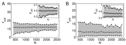
Figure 2: Mean values (squares) and range (shaded areas) of turning points $\varepsilon_{crit}$ in 200 independent realizations of the Lorenz (A) and the Rössler system (B) in dependence on the network size $N$ (Euclidean distance, $\Delta t=0.05$). The insets show the corresponding link densities $\rho_{crit}$ for the same range of $N$.

(iii) One has to emphasize that the turning point criterion is not generally applicable, since there are various typical examples for both discrete and continuous dynamical systems that are characterized by several maxima of $d\rho(\varepsilon)/d\varepsilon$ (Fig. 3).

The above considerations are mainly of concern when studying properties of (known) dynamical systems. In applications to real-world time series with typically a small number of data or even non-stationarities, it is still possible to derive meaningful qualitative results from small time series networks. However, for a detailed system-theoretic interpretation the use of smaller recurrence thresholds is recommended Marwan2009 .

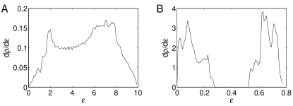
Figure 3: Examples for multiple turning points of $d\rho/d\varepsilon$: (A) quasiperiodic trajectory of a continuous system (torus) and (B) a weakly chaotic orbit of the standard map ($x_{n+1}=x_{n}+5\sin(y_{n})\mod 1$, $y_{n+1}=y_{n}+x_{n+1}\mod 1$, see Zou2007 ).

Topology of recurrence networks.

The topological features of recurrence networks are closely related to invariant properties of the observed dynamical system Marwan2009 ; Donner2009 ; Gao2009 . However, a system-theoretic interpretation of the resulting network characteristics is feasible only based on a careful choice of $\varepsilon$, avoiding the pitfalls outlined above. For example, many paradigmatic network models as well as real-world systems have been reported to possess small-world properties (i.e., a high clustering coefficient $\mathcal{C}$ and low average path length $\mathcal{L}$). However, it can be shown that $\mathcal{C}$ and $\mathcal{L}$ are both functions of $\varepsilon$. In particular, $\mathcal{L}\sim 1/\varepsilon$ (for given $N$), since spatial distances are approximately conserved in recurrence networks, whereas the specific $\varepsilon$-dependence of $\mathcal{C}$ varies between different systems.

In addition to the aforementioned global network characteristics, specific vertex properties characterize the local attractor geometry in phase space in some more detail, where the spatial resolution is determined by $\varepsilon$. In particular, the local clustering coefficient $\mathcal{C}_{v}$, which quantifies the relative amount of triangles centered at a given vertex $v$, gives important information about the geometric structure of the attractor within the $\varepsilon$-neighborhood of $v$ in phase space. Specifically, if the neighboring states form a lower-dimensional subset than the attractor, it is more likely that closed triangles emerge than for a neighborhood being more uniformly filled with states Dall2002 . Hence, high values of $\mathcal{C}_{v}$ indicate lower-dimensional structures that may correspond to laminar regimes Marwan2009 or dynamically invariant objects like unstable periodic orbits (UPOs) Donner2009 . The relationship with UPOs follows from the fact that trajectories tend to stay in the vicinity of such orbits for a finite time Lathrop_pra_1989 , which leads to a certain amount of states being accumulated along the UPO with a distinct spatial geometry that differs from that in other parts of a chaotic attractor. However, since there are infinitely many UPOs embedded in chaotic attractors, such objects (even of a low order) can hardly be detected using large $\varepsilon$ (where the resulting neighborhoods cover different UPOs) and short time series as recently suggested Gao2009 . In contrast, they may be well identified using low $\varepsilon$ and long time series Donner2009 .

Another intensively studied vertex property is betweenness centrality $b_{v}$, which quantifies the relative number of shortest paths in a network that include a given vertex $v$ Freeman1979 . In a recurrence network, vertices with high $b_{v}$ correspond to regions with low phase space density that are located between higher density regions. Hence, $b_{v}$ yields information about the local fragmentation of an attractor. In particular, since phase space regions close to the outer boundaries of the corresponding attractors do not contribute to many shortest paths, the vertices located in these regions are characterized by low $b_{v}$, which is (at least for the Lorenz oscillator) even enhanced by a lower state density. For the sharp inner boundary of the Rössler oscillator, one may observe the opposite behavior. For phase space regions close to low-period UPOs, one also finds lower values of $b_{v}$ due to the accumulation of states along these structures (many alternative paths). As the distribution of $b_{v}$ (Fig. 4 (A,B)) suggests, these features are robust for low $\varepsilon$, but may significantly change if $\varepsilon$ gets too large (i.e., $\rho=0.2$).

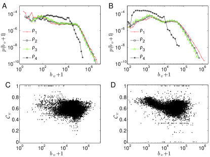
Figure 4: (Color online) Probability distribution function of betweenness centrality $b_{v}$ (in logarithmic scale) for different edge densities ($\rho_{1}=0.005$, $\rho_{2}=0.01$, $\rho_{3}=0.015$, $\rho_{4}=0.2$) for the Lorenz (A, $N=20,000$) and Rössler system (B, $N=10,000$), and corresponding relationships between local clustering coefficient $\mathcal{C}_{v}$ and betweenness centrality $b_{v}$ (C: Lorenz, D: Rössler, $\rho=0.01$) obtained from the original data using the Euclidean distance ($\Delta t=0.05$).

We conclude that in a recurrence network, both $\mathcal{C}_{v}$ and $b_{v}$ are sensitive to the presence of UPOs, but resolve complementary aspects (see Fig. 4). For the Rössler system, we find two distinct maxima in the betweenness distribution, which are related to the inner and outer parts of the attractor, respectively. In particular, the abundance of low values is promoted by a high state density at the outer boundary of the attractor near the $x$-$y$ plane, which coincides with a period-3 UPO Thiel2003 . In contrast, for the Lorenz system there is no second maximum of $p(b_{v})$, since the outer parts of the attractor are more diffuse and characterized by a considerably lower phase space density than in the Rössler attractor. In both cases, vertices with a high clustering coefficient $\mathcal{C}_{v}$ are characterized by a broad continuum of betweenness values, which suggests that $b_{v}$ is no universal indicator for the presence of UPOs, whereas $\mathcal{C}_{v}$ allows an approximate detection of at least low-periodic UPOs in phase space.

In summary, transforming time series into complex networks yields complementary measures for characterizing phase space properties of dynamical systems. This work has provided empirical arguments that the recently suggested approach based on the recurrence properties in phase space allows a detailed characterization of dynamically relevant aspects of phase space properties of the attractor, given that (i) the considered time series is long enough to be representative for the system’s dynamics and (ii) the threshold distance $\varepsilon$ in phase space for defining a recurrence is chosen small enough to resolve the scales of interest. In particular, using the network-theoretic measures discussed here, the turning point criterion for threshold selection Gao2009 often does not allow feasible conclusions about dynamically relevant structures in phase space. In contrast, for sufficiently low recurrence thresholds (we suggest $\rho\lesssim 0.05$ as a rule of thumb), small-scale structure may be resolved appropriately by complex network measures, which allow identification of invariant objects such as UPOs by purely geometric means. We emphasize that although our presented considerations have been restricted to paradigmatic example systems, recurrence networks and related methods have already been successfully applied to real-world data, e.g., a paleoclimate record Marwan2009 or seismic activity Davidsen2008 . Since these examples are typically characterized by non-stationarities and non-deterministic components, we conclude that recurrence networks are promising for future applied research on various interdisciplinary problems (e.g., Perc2005 ).

As a final remark, we note that the problem of parameter selection arises for most other network-based methods of time series analysis (see Donner2009 for a detailed comparison). Important examples include cycle networks Zhang2006 with a correlation threshold, and $k$-nearest neighbor networks Xu2008 with a fixed number $k$ of neighbors as free parameters, respectively. A general framework for parameter selection in the context considered here would consequently be desirable. Other methods are parameter-free, but may suffer from conceptual limitations and strong intrinsic assumptions. For example, the currently available visibility graph concepts Lacasa2008 are restricted to univariate time series.

Acknowledgments. This work has been financially supported by the German Research Foundation (SFB 555, project C4 and DFG project no. He 2789/8-2), the Max Planck Society, the Leibniz Society (project ECONS), and the Potsdam Research Cluster PROGRESS (BMBF). All complex networks measures have been calculated using the igraph package Csardi2006 .

References

- (1) R. Albert and A.-L. Barabási, Rev. Mod. Phys. 74, 47 (2002). M.E.J. Newman, SIAM Rev. 45, 167 (2003). A. Arenas, A. Díaz-Guilera, J. Kurths, Y. Moreno, and C.S. Zhou, Phys. Rep. 469, 93 (2008).
- (2) J.M. Montoya, S.L. Pimm, and R.V. Solé, Nature 442, 259 (2006).
- (3) L.C. Freeman, Soc. Netw. 1, 215 (1979).
- (4) C.S. Zhou, L. Zemanová, G. Zamora, C.C. Hilgetag, and J. Kurths, Phys. Rev. Lett. 97, 238103 (2006).
- (5) J.F. Donges, Y. Zou, N. Marwan, and J. Kurths, Eur. Phys. J. ST 174, 157 (2009), Europhys. Lett. 87, 48007 (2009).
- (6) J. Zhang, M. Small, Phys. Rev. Lett. 96, 238701 (2006).
- (7) N. Marwan, J.F. Donges, Y. Zou, R.V. Donner, and J. Kurths, Phys. Lett. A 373, 4246 (2009).
- (8) R.V. Donner, Y. Zou, J.F. Donges, N. Marwan, and J. Kurths, arXiv:0908.3447 [nlin.CD].
- (9) J.-P. Eckmann, S. Oliffson Kamphorst, and D. Ruelle, Europhys. Lett. 5, 973 (1987).
- (10) N. Marwan, M.C. Romano, M. Thiel, and J. Kurths, Phys. Rep. 438, 237 (2007).
- (11) X. Xu, J. Zhang, and M. Small, PNAS 105, 19601 (2008).
- (12) Z. Gao and N. Jin, Phys. Rev. E 79, 066303 (2009). Z. Gao and N. Jin, Chaos 19, 033137 (2009).
- (13) S. Schinkel, O. Dimigen, and N. Marwan, Eur. Phys. J. ST 164, 45 (2008).
- (14) A. Facchini and H. Kantz, Phys. Rev. E 75, 036215 (2007).
- (15) Y. Zou, M. Thiel, M.C. Romano, and J. Kurths, Chaos 17, 043101 (2007).
- (16) J. Dall and M. Christensen, Phys. Rev. E 66, 016121 (2002).
- (17) D. Lathrop and E. Kostelich, Phys. Rev. A 40, 4028 (1989).
- (18) M. Thiel, M.C. Romano, and J. Kurths, Appl. Nonlin. Dyn. 11, 20 (2003).
- (19) J. Davidsen, P. Grassberger, and M. Paszuski, Phys. Rev. E 77, 066104 (2008).
- (20) L. Lacasa, B. Luque, F. Ballesteros, J. Luque, and J.C. Nuño, PNAS 105, 4972 (2008).
- (21) M. Perc, Eur. J. Phys. 26, 525 (2005).
- (22) G. Csárdi and T. Nepusz, InterJournal CX.18, 1695 (2006).