Finite-Temperature Properties across the Charge Ordering Transition
– Combined Bosonization, Renormalization Group, and Numerical Methods –

Abstract

We theoretically describe the charge ordering (CO) metal-insulator transition based on a quasi-one-dimensional extended Hubbard model, and investigate the finite temperature ($T$) properties across the transition temperature, $T_{\rm CO}$. In order to calculate $T$ dependence of physical quantities such as the spin susceptibility and the electrical resistivity, both above and below $T_{\rm CO}$, a theoretical scheme is developed which combines analytical methods with numerical calculations. We take advantage of the renormalization group equations derived from the effective bosonized Hamiltonian, where Lanczos exact diagonalization data are chosen as initial parameters, while the CO order parameter at finite-$T$ is determined by quantum Monte Carlo simulations. The results show that the spin susceptibility does not show a steep singularity at $T_{\rm CO}$, and it slightly increases compared to the case without CO because of the suppression of the spin velocity. In contrast, the resistivity exhibits a sudden increase at $T_{\rm CO}$, below which a characteristic $T$ dependence is observed. We also compare our results with experiments on molecular conductors as well as transition metal oxides showing CO.

1 Introduction

Charge ordering (CO) phase transition is now found ubiquitously in strongly correlated electron systems such as transition metal oxides [1] and molecular conductors [2]. Its intuitive picture is simple: Electrons arrange spontaneously which results in lowering of the symmetry from the underlying lattice structure, in order to gain repulsive Coulomb energy as in Wigner crystals. Nevertheless, the richness of this phenomenon is now widely recognized, owing to extensive experimental as well as theoretical investigations in many types of compounds with different lattice geometries.

From the theoretical point of view, in spite of numerous studies [3], there remains a fundamental question not fully clarified yet, i.e., how the physical properties across the CO phase transition temperature ($T$), $T_{\rm CO}$, can be described. Typical mean-field analysis fails in reproducing finite-$T$ phase transitions from a metallic state to paramagnetic insulating CO states, which are, however, often observed in many strongly correlated electronic materials. Therefore, treatments beyond the simple mean-field approximation, which consider the effects of quantum fluctuation more properly, are necessary to describe such properties.

In general, one-dimensional (1D) models can be treated by taking the quantum fluctuations into account in a controlled way, compared to higher dimensional systems, by numerical as well as analytical methods. In fact, to describe CO in quarter-filled systems, the 1D extended Hubbard model (EHM) including the repulsive Coulomb interactions of onsite, $U$, and intersite, $V$, has intensively been studied. Especially, its ground-state properties (see Fig. 1) are known in detail; a quantum phase transition occurs between the metallic Tomonaga-Luttinger (TL) liquid state characterized by the TL liquid parameter $K_{\rho}$, and the CO insulating state ($T_{\rm CO}=0$) [3, 4, 5]. However, the 1D model does not show any phase transition at finite $T$ due to the enhanced low-dimensional fluctuations.

On the other hand, the two-dimensional (2D) square lattice EHM at quarter-filling shows finite $T_{\rm CO}$. Different techniques beyond the mean-field approximation have been applied to investigate the finite-$T$ properties of this model, such as exact diagonalization (ED) [6], slave-boson [7], dynamical mean-field [8, 9], correlator projection [10], and quantum Monte Carlo (QMC) [11] methods. However, due to theoretical difficulties, the physical properties across $T_{\rm CO}$ such as the spin susceptibility and the electrical resistivity are not elucidated, and the interplay between spin and charge degrees of freedom is not fully explored yet.

In this context, the quasi-1D (Q1D) EHM, i.e., 1D EHM chains coupled by the interchain Coulomb interaction $V_{\perp}$, has recently been studied by analytical [12, 13] as well as numerical [14, 15] methods by the present authors and co-workers, which shows a finite-$T$ CO phase transition with concomitant metal-insulator transition at quarter-filling. In these studies, the interchain mean-field treatment [16] is applied and the resultant effective 1D model is solved using different methods which properly take into account the large fluctuation effects: by the bosonization + renormalization group (RG) scheme in refs. YTS2006 and YTS2007, and by numerical techniques, i.e., the quantum transfer-matrix method in ref. Seo2007 and the QMC method in ref. Otsuka2008.

In the former analytical approach, which has the advantage in investigating the critical regions, it is found that the $V_{\perp}$-term considerably affects the stability of the CO state compared with that in the 1D EHM [12]. Due to the dimensionality effect, $T_{\mathrm{CO}}$ always becomes finite whenever the CO phase is realized, except for the critical point (line). Then, the ground state phase diagram of the 1D EHM on the $U$-$V$ plane is divided into three regions depending on the TL liquid parameter $K_{\rho}$, as in Fig. 1. They show different properties when $V_{\perp}$ is turned on:

• Region (i) [$K_{\rho}>1/2$] Finite value of $V_{\perp}$ is necessary to produce the CO state.

• Region (ii) [$1/4\leq K_{\rho}\leq 1/2$] Infinitesimal $V_{\perp}$ turns the system from TL liquid to CO insulator with finite $T_{\mathrm{CO}}$.

• Region (iii) [$K_{\rho}$ is not defined (CO insulating ground state for $V_{\perp}=0$)] Infinitesimal $V_{\perp}$ makes $T_{\mathrm{CO}}$ finite.

Therefore, once $V_{\perp}$ is added, the CO phase critically enlarges from region (iii) to regions (ii)+(iii). In addition, the effects of the lattice dimerization along the chain direction and the frustration in the interchain interactions on the above Q1D model have been studied [13]; the lattice dimerization suppresses $T_{\mathrm{CO}}$, and the interchain frustration leads to a competition between CO states with different charge patterns [17].

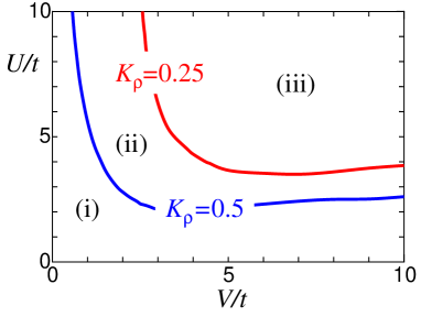
Figure 1: (Color online) Phase diagram of the quasi-one-dimensional extended Hubbard model, obtained by the interchain mean-field theory [12]. In region (i), the CO state is stabilized when $V_{\perp}>V_{\perp}^{\mathrm{c}}$ with finite $V_{\perp}^{\mathrm{c}}>0$. In region (ii), infinitesimal $V_{\perp}$ changes the TL liquid state at $V_{\perp}=0$ into the CO state. In region (iii), where the CO state is obtained even in the purely 1D case, the CO state is obtained at finite temperature by the interchain coupling. The boundary between (i) and (ii), and that between (ii) and (iii) are characterized by the value of $K_{\rho}=1/2$ and that of $K_{\rho}=1/4$ for the 1D model.

In these studies, although the finite-$T$ properties above $T_{\rm CO}$ are elucidated by taking advantage of the RG treatment which we will describe later, properties below $T_{\rm CO}$ were hardly investigated due to difficulties in determining the CO order parameter in a self-consistent manner. Meanwhile, the ‘initial’ values in the RG equations were taken as the bare TL parameters derived from weak-coupling expansions of the EHM; such a procedure loses accuracy in general when the interaction becomes large. Nevertheless, this drawback is not due to the phase Hamiltonian representation by the bosonization method nor the RG approach; it is because of the choice of the initial condition for the RG equations.

On the other hand, the numerical quantum transfer matrix and QMC methods used in refs. Seo2007 and Otsuka2008 are suitable for the intermediate-to-strong coupling regime; by applying the interchain mean-field approach as well, the Q1D EHM and its extensions with different types of electron-lattice interaction are treated. Competitions and co-existences among different states, including the paramagnetic CO insulator, are clarified, and the $T$ dependences of different order parameters as well as the charge and spin susceptibilities across the transition temperatures are computed. In particular, the QMC method could provide highly accurate results down to considerably low $T$. However, there are quantities which cannot be calculated by such numerical simulations directly, such as the electrical resistivity: one of the most basic information from experiments.

Up to now, the above-mentioned analytical and numerical approaches for the Q1D quarter-filled electron systems have been separately employed, being complimentary to each other. In the present study, in contrast, we develop a combined method. The numerical ED data are implemented into the analytical bosonization + RG scheme, as initial conditions of the RG equations [18]. As for the properties below $T_{\mathrm{CO}}$, the $T$ dependence of the CO order parameter is calculated by the QMC method [15], and then adopted to the scheme above. This combined method enables us to compute the $T$ dependences of physical properties such as the spin susceptibility and the electrical resistivity across $T_{\mathrm{CO}}$.

The organization of this paper is as follows. In §2, our combined analytical and numerical method applied to the Q1D EHM is formulated. In §3, the $T$ dependences of the physical quantities across the CO transition are shown. Section 4 is devoted to the summary and discussions, including comparisons with experiments on different CO materials. Detailed description of our theoretical approach is presented in Appendix A, and a benchmark check of this method applied to the 1D Hubbard model is given in Appendix B.

2 Formulation

In this section, the model and formulation for our calculation are given. In § 2.1, first we explain the interchain mean-field approach to the Q1D EHM and the bosonization + RG method applied to the effective 1D model, which were partly formulated in refs. YTS2006 and YTS2007. Then, in § 2.2 we explain how the numerical techniques are combined with this method.

2.1 Bosonization + RG

The Q1D EHM that we study consists of quarter-filled 1D extended Hubbard chains coupled by the interchain interaction $V_{\perp}$. [12] The Hamiltonian $H_{\mathrm{Q1D}}$ is given by

$$H_{\mathrm{Q1D}} =\sum_{j}H^{j}_{\mathrm{1D}}+H_{\perp},$$ (1)

$$H^{j}_{\mathrm{1D}}= -t\sum_{i,s}\left(c^{\dagger}_{i,j,s}c_{i+1,j,s}+\mathrm{h.c.}\right)$$

$$+U\sum_{i}n_{i,j,\uparrow}\,n_{i,j,\downarrow}+V\sum_{i}n_{i,j}\,n_{i+1,j},$$ (2)

$$H_{\perp} =V_{\perp}\sum_{i,\langle j,j^{\prime}\rangle}n_{i,j}\,n_{i,j^{\prime}},$$ (3)

where $H^{j}_{\mathrm{1D}}$ and $H_{\perp}$ represent the 1D EHM of the $j$-th chain and the interchain-coupling term, respectively. Here, $t$ is the transfer integral between the nearest-neighbor sites along the chain direction; we do not consider the interchain hopping energy here. The operator $c^{\dagger}_{i,j,s}$ creates an electron with spin $s=\uparrow$ or $\downarrow$ at the $i$-th site in the $j$-th chain. The density operators are defined as $n_{i,j,s}=c^{\dagger}_{i,j,s}c_{i,j,s}-1/4$ and $n_{i,j}=n_{i,j,\uparrow}+n_{i,j,\downarrow}$.

The interchain coupling term is treated within the interchain mean-field approximation [16] as

$$H_{\bot}\simeq V_{\bot}\sum_{i,\langle j,j^{\prime}\rangle}\left(\langle n_{i,j}\rangle n_{i,j^{\prime}}+n_{i,j}\langle n_{i,j^{\prime}}\rangle-\langle n_{i,j}\rangle\langle n_{i,j^{\prime}}\rangle\right).$$ (4)

Assuming the Wigner-crystal-type CO with two-fold periodicity, we postulate $\langle n_{i,j}\rangle=(-1)^{i+j}n$ where $n$ is the CO order parameter [12]. After this procedure, we obtain an effective 1D Hamiltonian:

$$H= -t\sum_{i,s}\left(c^{\dagger}_{i,s}c_{i+1,s}+\mathrm{h.c.}\right)$$

$$+U\sum_{i}n_{i,\uparrow}\,n_{i,\downarrow}+V\sum_{i}n_{i}\,n_{i+1}$$

$$+zV_{\perp}n\sum_{i}(-1)^{i}n_{i}+\frac{1}{2}zLV_{\bot}n^{2},$$ (5)

where the chain index is omitted. The number of the sites in the chain and that of the adjacent chains are expressed as $L$ and $z$, respectively.

By the bosonization method, the effective 1D Hamiltonian eq. (5) can be expressed in terms of the bosonic fields. Then the Hamiltonian is separated into the charge part $\mathcal{H}_{\rho}$ and the spin part $\mathcal{H}_{\sigma}$ as

$$H= \int{\rm d}x(\mathcal{H}_{\rho}+\mathcal{H}_{\sigma})+\frac{1}{2}zLV_{\bot}n^{2},$$ (6)

$$\mathcal{H}_{\rho}= \frac{v_{\rho 0}}{4\pi}\left[\frac{1}{K_{\rho 0}}(\partial_{x}\theta_{\rho})^{2}+K_{\rho 0}(\partial_{x}\phi_{\rho})^{2}\right]$$

$$+\frac{g_{3\bot}}{(\pi\alpha)^{2}}\cos 2\theta_{\rho}+\frac{g_{1/4}}{2(\pi\alpha)^{2}}\cos 4\theta_{\rho},$$ (7)

$$\mathcal{H}_{\sigma}= \frac{v_{\sigma 0}}{4\pi}\left[\frac{1}{K_{\sigma 0}}(\partial_{x}\theta_{\sigma})^{2}+K_{\sigma 0}(\partial_{x}\phi_{\sigma})^{2}\right]$$

$$+\frac{g_{1\bot}}{(\pi\alpha)^{2}}\cos 2\theta_{\sigma},$$ (8)

where the phase variables satisfy $[\theta_{\mu}(x),\phi_{\nu}(x^{\prime})]={\rm i}\pi\mathrm{sgn}(x-x^{\prime})\delta_{\mu\nu}$ with $\mu,\nu=\rho$ or $\sigma$, and $\alpha$ is a short-distance cutoff. The parameters $K_{\rho 0}$ ($K_{\sigma 0}$) and $v_{\rho 0}$ ($v_{\sigma 0}$) are the bare TL-liquid parameter and velocity for the charge (spin) degree of freedom, respectively. They take non-universal values depending on the strength of interactions.

In the charge sector, $\mathcal{H}_{\rho}$, there appear two kinds of non-linear terms. The term proportional to $\cos 4\theta_{\rho}$ originates from the $8k_{\rm F}$ umklapp scattering [$k_{\rm F}(=\pi/4)$ is the Fermi momentum], whose coupling constant $g_{1/4}$ is finite even in the purely 1D EHM and it leads to the CO insulating ground state [4, 19, 20]. On the other hand, the $\cos 2\theta_{\rho}$ term represents the $4k_{\rm F}$ umklapp scattering process, whose coupling constant $g_{3\perp}$ is proportional to $n$ when $|g_{3\bot}|\ll\pi v_{\rho 0}$ [12]. This $4k_{\rm F}$ umklapp scattering process is generated in the existence of CO, which can be understood by noting that the one-particle energy gap opens at $\pm 2k_{\rm F}$ because of the two-fold periodicity in the CO state and then the conduction band becomes effectively half filled.

The spin part $\mathcal{H}_{\sigma}$ is essentially the same as the effective Hamiltonian of the Heisenberg chain. The parameters $K_{\sigma 0}$ and $g_{1\bot}$ in eq. (8) are not independent because of the spin-rotational SU(2) symmetry:

$$K_{\sigma 0}=\sqrt{\frac{\pi v_{\sigma 0}+g_{1\bot}}{\pi v_{\sigma 0}-g_{1\bot}}}.$$ (9)

This constraint still holds even under the scaling procedure. In the low-energy limit, the $g_{1\perp}$ coupling is renormalized to zero and $K_{\sigma 0}$ reduces to unity. When the system has the SU(2) symmetry, it is known that physical quantities exhibit logarithmic (very slow) system-size or $T$ dependences due to the presence of marginal operators.[21] These characteristics can be captured by the RG analysis.

The RG equations for the charge part $\mathcal{H}_{\rho}$ [eq. (7)] are given by

$$\frac{{\rm d}}{{\rm d}l}K_{\rho}(l) =-2G_{3\bot}^{2}(l)\,K_{\rho}^{2}(l)-8G_{1/4}^{2}(l)\,K_{\rho}^{2}(l),$$ (10)

$$\frac{{\rm d}}{{\rm d}l}G_{3\bot}(l) =(2-2K_{\rho}(l))G_{3\bot}(l)-G_{3\bot}(l)\,G_{1/4}(l),$$ (11)

$$\frac{{\rm d}}{{\rm d}l}G_{1/4}(l) =(2-8K_{\rho}(l))G_{1/4}(l)-\frac{1}{2}G_{3\bot}^{2}(l).$$ (12)

We note that, in ref. YTS2006, the above equations with $G_{3\bot}(l)=0$ ($g_{3\bot}=0$) were treated, corresponding to the absence of CO order parameter $n$, to investigate the instability toward $T_{\rm CO}$. As for the spin part, the scaling equation for the coupling in $\mathcal{H}_{\sigma}$ [eq. (8)] is

$$\frac{{\rm d}}{{\rm d}l}G_{1\bot}(l)=-2G_{1\bot}^{2}(l)-2G_{1\bot}^{3}(l),$$ (13)

and $K_{\sigma}(l)$ is determined as

$$K_{\sigma}(l)=\sqrt{\frac{1+G_{1\bot}(l)}{1-G_{1\bot}(l)}},$$ (14)

following eq. (9). In the usual analysis, to obtain the parameters $\{K_{\rho}(l),G_{3\bot}(l),G_{1/4}(l)\}$ for the charge part and $G_{1\bot}(l)$ for the spin part as the solutions of the RG equations, the initial conditions are set from the bare parameter values as $K_{\rho}(0)=K_{\rho 0}$, $G_{3\perp}(0)=g_{3\perp}/(\pi v_{\rho 0})$, $G_{1/4}(0)=g_{1/4}/(2\pi v_{\rho 0})$, and $G_{1\perp}(0)=g_{1\perp}/(\pi v_{\sigma 0})$. Such initial values can be calculated from the parameters of the original lattice model by considering the interaction processes near the Fermi level. In our previous studies on CO based on such procedure [4, 22, 12, 13], the third-order processes mediated by the states far from the Fermi level were crucial in deriving the $8k_{\rm F}$ umklapp scattering $g_{1/4}$-term, which triggers the CO insulating state. Note that the third-order virtual processes also play crucial roles for the spin degree of freedom [4].

We also note that the RG equations above for the charge part are shown up to the one-loop level, while, on the other hand, that for the spin coupling $G_{1\perp}(l)$ is shown up to the two-loop level, i.e., $O(G_{1\perp}^{3})$. Since there are subtleties in deriving the two-loop RG equation based on the bosonized Hamiltonian, we follow the consideration given in ref. Emery and use the RG equation for $G_{1\perp}$ based on the Hamiltonian for the original fermion variables.

When we apply the RG method to systems at finite $T$, the assumption of the scaling invariance breaks down and the RG scaling is cut off at the scale $l$ corresponding to the temperature $T$: $l\simeq l_{T}\equiv\ln(Ct/T)$ with $C$ being an $O(1)$ numerical constant. Then we can discuss the finite-$T$ properties by terminating the scaling procedure at $l_{T}$, and use the values $\{K_{\rho}(l_{T}),G_{3\bot}(l_{T}),G_{1/4}(l_{T})\}$ and $G_{1\bot}(l_{T})$ as the $T$-dependent quantities; we write them as $\{K_{\rho}(T),G_{3\bot}(T),G_{1/4}(T)\}$ and $G_{1\bot}(T)$ in the following. These $T$-dependent parameters are set in the formulae for the physical quantities, as will be discussed in § 3.

2.2 Numerical methods

The procedure of setting the initial conditions of the RG equation mentioned above, i.e., to derive them based on the perturbation theory, generally looses accuracy in the strong-coupling region. For example, the ground state phase diagram of the 1D EHM obtained in this way qualitatively agrees with the other numerical methods in the weak-coupling region, while the phase boundary between TL liquid and CO insulator deviates at strong-coupling [4]. In the present study, instead, in order to obtain more accurate results even for stronger interactions, we make use of numerical data for finite size systems, as discussed in the following. Such an approach was recently proposed in ref. Sano2004 to investigate the charge degree of freedom of the 1D EHM, which reproduced the ground-state phase diagram with high accuracy. Here we extend their method in order to calculate the finite-$T$ properties by solving the RG equations in § 2.1 and stopping the scaling at $l_{T}$ as mentioned above.

For small systems with sites $L$, the TL parameters $K_{\rho}^{L}$ and $K_{\sigma}^{L}$ can be computed by the Lanczos ED technique directly applied to the lattice Hamiltonian eq. (5). These can be used as initial values of the RG equations by taking advantage of the relation between the scaling variable $l$ and the system size, $l\simeq\ln{L}$ (in the calculation we use $l=\ln{L}$ since the deviation is small for a different factor ). For the charge part, eqs. (10)-(12), where the three parameters $\{K_{\rho}(l),G_{3\bot}(l),G_{1/4}(l)\}$ are coupled in the form of differential equations, we can set $K_{\rho}^{L}$ for available system sizes as initial values by fitting them to the RG equations to determine the solutions. As for the spin degree of freedom, the initial value for $G_{1\bot}(l)$ in eq. (13) is determined from $K_{\sigma}^{L}$ using the relation eq. (9). It will be discussed in § 3.1 that, for the calculation of the spin susceptibility, we also make use of $T$-dependent spin velocity $v_{\sigma}(T)$. However, the spin velocity cannot be determined reliably from the RG flow due to subtleties in deriving its RG equation. Therefore, instead, we use the standard polynomial finite size scaling for several system sizes $L$ and extrapolate it to the size corresponding to $\ln{L}\simeq l_{T}$, which provides $v_{\sigma}(T)$. More detailed procedure for determining the $T$-dependent parameters using the Lanczos ED data is given in Appendix A.

We also combine numerical data for the CO order parameter $n$. It is finite for $T<T_{\rm CO}$, which affects the parameters of the system; especially $g_{3\bot}$ ($G_{3\bot}$) becomes finite when $n$ $\neq$ 0. However, its $T$ dependence cannot be obtained within the bosonization + RG scheme in a self-consistent manner, due to the ambiguity in the relationship between $n$ and the phase variable [24]. In order to overcome this difficulty, in the present study, $n$ is numerically obtained by the QMC method in advance, and adopted to the above scheme. We employ the stochastic-series-expansion (SSE) method [25, 26] with the operator-loop update [27, 28] as a solver for the effective 1D lattice Hamiltonian (5). At each $T$, the order parameter is iteratively calculated by this QMC method until it converges [15]. We calculate systems with sizes up to $L=128$ sites and checked that finite size effects are negligible down to low $T$ that we discuss in this paper. The results are substituted into eq. (5) and treated as an ‘external field’, which reflect the initial values of the RG equations.

Summarizing, at each $T$, first the value of $n$ is calculated by QMC, and then the initial conditions of the RG equations are collected using Lanczos ED by substituting the QMC data into the lattice Hamiltonian, and finally the RG equations (and the usual finite size scaling for the spin velocity) are solved by stopping the scaling at the scale $l$ corresponding to the temperature $T$. This provides the finite-$T$ values of the parameters to be input in the expressions of the physical quantities which will be described in the next section.

3 Temperature Dependences of Spin Susceptibility and Electrical Resistivity

In this section, the $T$ dependences of the spin susceptibility $\chi_{\sigma}(T)$ and the electrical resistivity $\rho(T)$ are discussed. We focus on the regions (ii) and (iii) in Fig. 1 and study how the physical quantities behave for wide $T$ ranges across $T_{\rm CO}$. For the intrachain parameter, we set $(U/t,V/t)=(6.0,\,2.5)$ for the region (ii) and $(10.0,\,4.0)$ for the region (iii).

3.1 Uniform spin susceptibility

The formula for the uniform spin susceptibility $\chi_{\sigma}(T)$ in the RG scheme has been derived in refs. Nelisse1999 and Fuseya2005. The naive random-phase-approximation (RPA) gives $\chi_{\sigma}^{\mathrm{RPA}}(T)=[2\chi_{0}(T)/{\pi v_{F}}]/[1-U\chi_{0}(T)/(\pi v_{F})]$, where $v_{F}$ is the Fermi velocity and $\chi_{0}(T)$ is the spin susceptibility in the non-interacting case normalized as $\chi_{0}(0)=1$. On the other hand, when the 1D fluctuation effects are taken into account by the RG method, it is written as [29, 30],

$$\chi_{\sigma}(T)=\frac{2}{\pi v_{F}}\frac{\chi_{0}(T)}{1-\left[G_{1\bot}(T)+G_{4\sigma}(T)\right]\chi_{0}(T)}.$$ (15)

Here, $G_{1\bot}(T)$ is the amplitude of the backward scattering, which is obtained by the RG scheme in § 2. The coupling $G_{4\sigma}(T)$, on the other hand, represents the same-branch forward scattering in the spin channel. [29]. It reflects the velocity of the spin excitations through the relation

$$G_{4\sigma}(T)=1-\frac{v_{\sigma}(T)}{v_{F}},$$ (16)

then we can use the $T$-dependent spin velocity $v_{\sigma}(T)$ obtained by the finite size scaling introduced in § 2. We note that eqs. (15) and (16) reproduce the correct formula $\chi_{\sigma}(0)=2/[\pi v_{\sigma}(0)]$ in the $T\to 0$ limit. In refs. Nelisse1999 and Fuseya2005, the linearized dispersion was used in deriving the noninteracting susceptibility $\chi_{0}(T)$. Here, instead, in order to analyze $\chi_{\sigma}(T)$ in a wider $T$ range, we use the dispersion of the tight-binding model to calculate $\chi_{0}(T)$ (see also Appendix B).

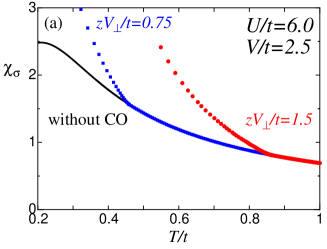
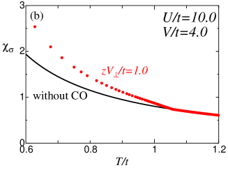
Figure 2: (Color online) $T$ dependence of the spin susceptibility $\chi_{\sigma}(T)$ (in the unit of $1/(ta)$), (a) for the region (ii) in Fig. 1[$(U/t,V/t)=(6.0,\,2.5)$] and (b) for the region (iii) [$(U/t,V/t)=(10.0,\,4.0)$]. The solid curve shows the data for $V_{\perp}=0$, without charge order at finite $T$.

In Fig. 2, the results are shown for regions (ii) and (iii), where, in both cases, $\chi_{\sigma}(T)$ is enhanced below $T_{\rm CO}$, without any steep singularity at $T=T_{\rm CO}$. The main reason for the enhancement is as follows. The CO order parameter $n$ induces a gap formation at $k=\pm 2k_{\rm F}=\pm\pi/2$ in the energy dispersion, and hence the density of states at the Fermi energy is increased (the Fermi velocity is suppressed). This leads to the suppression of the spin velocity.

The same approach can be applied to evaluate the splitting of Knight shift, which is often observed in experiments to detect the CO transition. In the interchain mean-field approach, the Knight shift at the charge rich site and the poor site, $S_{+}$ and $S_{-}$, are given by [13]

$$S_{\pm}\propto\chi_{\sigma}(T)\left[1\pm\frac{zV_{\perp}n}{\sqrt{2t^{2}+(zV_{\perp}n)^{2}}}\right].$$ (17)

For small $V_{\perp}n/t$, we obtain a simple relation $S_{\pm}\propto\chi_{\sigma}(T)[1\pm zV_{\perp}n/2t]$. Similarly, we can derive the formula of the nuclear relaxation rate, whose separation is also an experimental evidence of CO:

$$\frac{1}{(T_{1\pm})T}\propto\left[1\pm\frac{zV_{\perp}n}{\sqrt{2t^{2}+(zV_{\perp}n)^{2}}}\right]^{2},$$ (18)

where the relaxation rate at the charge rich and poor sites are denoted by $(T_{1+})^{-1}$ and $(T_{1-})^{-1}$, respectively. Note that the discrepancy in the order of the factor $1\pm zV_{\perp}n/\sqrt{2t^{2}+(zV_{\perp}n)^{2}}$ between (17) and (18) comes from the fact that the former expresses the local response under the uniform perturbation, whereas the latter is the local response under the local perturbation. Namely, $S_{i}\propto\sum_{i^{\prime}}\chi_{\sigma}(i,i^{\prime};0)$ and $(T_{1i}T)^{-1}\propto\lim_{\omega\to 0}{\rm Im}\chi_{\sigma}(i,i;\omega)/\omega$, where $S_{i}$ and $T_{1i}^{-1}$ are the Knight shift and the NMR relaxation rate at the $i$-th site, and $\chi_{\sigma}(i,i^{\prime};\omega)$ is the dynamical spin susceptibility in the site representation.

3.2 Electrical resistivity

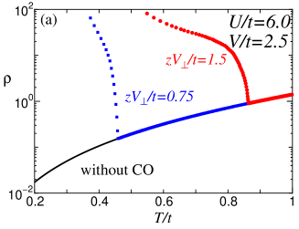
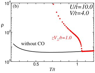
Figure 3: (Color online) $T$ dependence of the resistivity $\rho(T)$ in arbitrary unit, (a) for the region (ii) and (b) for the region (iii) [same parameters as in Fig. 2]. The solid curve shows the data for $V_{\perp}=0$, without charge order at finite $T$.

Next we discuss the $T$ dependence of the electrical resistivity $\rho(T)$. Based on the memory function approach, [31, 32] we perform the perturbation expansion with respect to $g_{3\perp}$ and $g_{1/4}$ in eq. (7) and then the formula for the resistivity is given by [22]

$$\rho(T)= \frac{1}{\pi v_{\rho 0}^{2}\alpha}\Bigg{[}g_{3\bot}^{2}\left(\frac{2\alpha}{\xi_{T}}\right)^{4K_{\rho 0}-3}B^{2}(K_{\rho 0},K_{\rho 0})$$

$$+g_{1/4}^{2}\left(\frac{2\alpha}{\xi_{T}}\right)^{16K_{\rho 0}-3}B^{2}(4K_{\rho 0},4K_{\rho 0})\Bigg{]},$$ (19)

where $B(x,y)=\Gamma(x)\Gamma(y)/\Gamma(x+y)$ is the beta function and $\xi_{T}=v_{\rho 0}/(\pi T)$ is the thermal coherence length. Here we note that the anomalous power-law behavior $G_{3\bot}^{2}T^{4K_{\rho}-4}$ and $G_{1/4}^{2}T^{16K_{\rho}-4}$ can already be seen from the perturbationaly-obtained form, eq. (19). However this expression is valid only in the high-$T$ region. In order to examine qualitative behaviors in the wide $T$ range, we reinforce these expressions within the RG framework. [31, 32] By noting that the scaling dimension of the $4k_{F}$ and $8k_{F}$ umklapp scatterings are $2K_{\rho 0}$ and $8K_{\rho 0}$, the couplings are scaled (at tree level) as $G_{3\bot}(l)=G_{3\bot}(0)\exp\left[(2-2K_{\rho 0})l\right]$ and $G_{1/4}(l)=G_{1/4}(0)\exp\left[(2-8K_{\rho 0})l\right]$. By inserting these relations into eq. (19), and replacing the bare parameter $K_{\rho 0}$ by the renormalized parameter $K_{\rho}(l)$, we obtain the formula improved by the RG method. Then the $T$ dependence can be computed as

$$\rho(T)= \frac{2\pi^{2}T}{v_{\rho 0}}\Bigg{[}G_{3\bot}^{2}(T)B^{2}(K_{\rho}(T),K_{\rho}(T))$$

$$\qquad+4G_{1/4}^{2}(T)B^{2}(4K_{\rho}(T),4K_{\rho}(T))\Bigg{]},$$ (20)

where the $T$-dependent coupling constants are obtained by the procedure in § 2.

In Fig. 3, we show the results of $\rho(T)$ thus calculated, for the regions (ii) and (iii). First, in the case of $V_{\perp}=0$ without CO at finite-$T$, the system shows a metallic behavior for the whole $T$ range for region (ii), i.e., $\rho(T)$ decreases with decreasing $T$, whereas for region (iii), it is insulating below the $T$ scale of the charge gap, i.e., $\rho(T)$ increases with decreasing $T$. This behavior reflects the ground-state properties in the absence of the interchain coupling, i.e., the TL liquid in the region (ii), while the CO insulating state in the region (iii). A noticeable point is that $\rho(T)$ shows insulating behavior even without long range order of CO [22] due to the low-dimensional fluctuation effect.

When $V_{\perp}\neq 0$, $T_{\rm CO}$ becomes finite, then one can see a clear cusp in $\rho(T)$ at $T=T_{\rm CO}$. Just below $T_{\rm CO}$, $\rho(T)$ shows a curve which is convex upward in the semi-log plot, reflecting the gap opening with the rapid growth of the CO order parameter $n$. At lower $T$, the curve turns convex downward, since at sufficiently low $T$, $n$ becomes almost $T$ independent and therefore the gap can be considered as a constant value, $\Delta$; then an activation-type behavior $\rho(T)\propto\exp{(\Delta/T)}$ is expected. Such a behavior is common for all the parameters we have considered, as shown in Fig. 3. The abrupt change at $T=T_{\rm CO}$ is indeed due to the emergence of 4$k_{\rm F}$-umklapp scattering which originates from the gap in the energy dispersion at $\pm 2k_{\rm F}$ owing to CO. This is in clear contrast with the behavior of the spin susceptibility $\chi_{\sigma}(T)$ shown in Fig. 2 with only a tiny singularity at the transition.

4 Summary and Discussions

In the present paper, we have formulated a new theoretical framework to investigate the finite-$T$ properties of Q1D electron systems. The method has been applied to the CO phase transition in the Q1D EHM at quarter filling, where extended Hubbard chains are coupled via interchain Coulomb repulsion treated within the interchain mean-field approximation.

In our scheme, we derive the bosonized Hamiltonian for the effective 1D model and treat the RG equations, and by stopping the scaling procedure at the corresponding scale we obtain finite-$T$ properties of the system. As for the initial values of the RG equations we use the numerical results for the small systems obtained by the Lanczos ED method; these provide quantitatively good estimates even for strong coupling regime, in contrast with the conventional treatment where only the interaction processes between electrons near the Fermi energy are taken into account. In addition, QMC method is employed to calculate $T$ dependence of the CO order parameter, which is necessary for the quantitative calculations below $T_{\rm CO}$ but difficult to determine in the bosonization + RG scheme. This framework enables us to calculate physical quantities across $T_{\rm CO}$ such as the spin susceptibility $\chi_{\sigma}(T)$ as well as the electrical resistivity $\rho(T)$ which is hard to calculate by the QMC simulation.

The results show that, CO leads to an enhancement of $\chi_{\sigma}(T)$, mainly due to the reduction of the spin velocity, but without any steep singularity at $T=T_{\rm CO}$. Such features in the $\chi_{\sigma}(T)$ curves shown in Fig. 2 are consistent with those calculated by purely numerical methods in refs. Seo2007 and Otsuka2008, which also showed a slight enhancement below $T_{\rm CO}$. In addition, our results share similarities with the $T=0$ properties of the 1D EHM, where $\chi_{\sigma}(T=0)$ shows no singular behavior at the critical value of $V$ for the emergence of CO, and continuously enhances when entering the CO phase [33]. On the other hand, as for $\rho(T)$, the CO phase transition results in a sudden increase with a change of the slope with decreasing $T$, due to the generation of 4$k_{\rm F}$-umklapp scattering which originates from the gap formation in the energy dispersion at $\pm 2k_{\rm F}$. This is the first theoretical work, to the authors’ knowledge, calculating $\rho(T)$ across the CO transition temperature starting from a microscopic correlated electronic model and taking full account of the quantum and thermal fluctuation effects.

Such results can be compared with the experiments, where $\chi_{\sigma}(T)$ and $\rho(T)$ are the most essential information for the bulk magnetic and electric properties of the system, measured most commonly. In fact, the sudden increase and the change of slope in $\rho(T)$ are observed in a wide classes of compounds showing CO, even in materials which are apparently not applicable to our Q1D model. On the other hand, there are differences in the behavior of $\chi_{\sigma}(T)$ at $T_{\rm CO}$ among the compounds, as discussed below. Nevertheless, in many materials no noticeable change is seen in $\chi_{\sigma}(T)$, indicating a transition to the paramagnetic insulating CO phase, as in our calculations.

For example, in quarter-filled molecular conductors where many compounds show CO, Q1D materials such as (TMTTF)${}_{2}X$ and (DCNQI)${}_{2}X$ (except the $\pi$-d mixed compound $X=$Cu) are candidates to be directly compared to our results, since ours can be considered as a microscopic model for their electronic properties. Several members of the (TMTTF)${}_{2}X$ family showing CO, such as $X$=SbF₆, AsF₆, and ReO₄, indeed show kinks at $T_{\rm CO}$ in their transport properties [34, 35]. A difference between our model and the situation in the actual TMTTF compounds is that, the present calculation does not include the intrinsic lattice dimerization along the chains while it exists in the materials, which leads to another non-linear term in the bosonized Hamiltonian [22]. In (DI-DCNQI)₂Ag, even though recent studies [36, 37] revealed that the system undergoes a more complex charge-lattice ordering than the simple CO we investigate in this paper, the $T$ dependence in $\rho(T)$ across $T=T_{\rm CO}$ observed at high pressure resembles our calculated data, whereas the kink at $T=T_{\rm CO}$ is smeared out at ambient pressure [38, 39]. All these Q1D molecular conductors show no anomaly in the bulk $\chi_{\sigma}(T)$ at $T=T_{\rm CO}$, while NMR measurements show the appearance of atomic sites showing different Knight shifts and relaxation rates [40, 41]: these are also consistent with our analysis. Recently, several Q1D compounds without dimerization have been synthesized where a CO transition is suggested, such as (o-DMTTF)₂Br [42] and (EDT-TTF-CONMe)${}_{2}X$ [$X$= AsF₆ and Br] [43, 44]. There, as in (DI-DCNQI)₂Ag at ambient pressure, the anomaly at $T=T_{\rm CO}$ in $\rho(T)$ is not clearly seen possibly due to the strong fluctuation which may be underestimated in our calculation due to the interchain mean-field treatment. A noticeable point is that in (o-DMTTF)₂Br [42], $\chi_{\sigma}(T)$ shows a steep decrease at around $T=T_{\rm CO}$, distinct from the other Q1D materials above with a smooth variation there, whose origin remains unclear.

Now there are many quasi-two-dimensional (Q2D) molecular conductors found to show CO. In such cases, the anomaly in $\rho(T)$ and the characteristic curvature below $T=T_{\rm CO}$ are again ubiquitously observed, while $\chi_{\sigma}(T)$ show different behaviors from material to material. The latter diversity is due to the fact that, in the Q2D compounds, there exists a variety in the anisotropy of transfer integrals originated from different molecular packings, which results in different anisotropic exchange couplings connecting the localized spins when CO is formed: For example, a spin gapped behavior is observed in $\alpha$-(BEDT-TTF)₂I₃ [45] and $\beta^{\prime\prime}$-(DODHT)₂PF₆ [46] due to the alternation in the exchange couplings along the charge rich sites. On the other hand, behavior analogous to our calculation is seen in $\theta$-(BDT-TTP)₂Cu(NCS)₂ [47, 48], where the $\rho(T)$ curve shows a rapid increase at around $T_{\rm CO}=250$ K, where $\chi_{\sigma}(T)$ shows no anomaly and below which the system is paramagnetic. In $\theta$-(BEDT-TTF)₂RbZn(SCN)₄, where the molecular packing in the 2D plane is the same, $\chi_{\sigma}(T)$ across $T_{\rm CO}=190$ K is also paramagnetic; however, in $\rho(T)$ a large jump is observed at $T=T_{\rm CO}$ [49]. The difference between the two $\theta$-type compounds is in their CO pattern: the ‘vertical stripe’ in the former and the ‘horizontal stripe’ in the latter. This results in different manners in coupling to the lattice degree of freedom, leading to the second-order vs strong first-order nature of the CO phase transition. We note that most of the Q2D compounds show a second-order or a weak first-order phase transition, and $\theta$-(BEDT-TTF)₂RbZn(SCN)₄ is rather exceptional. Another point we note here is that under pressure, in several Q2D compounds such as $\alpha$-(BEDT-TTF)₂I₃ [50] and $\beta$-(meso-DMBEDT-TTF)₂PF₆ [51, 52], $\rho(T)$ curve at low $T$ points toward a finite value extrapolated to $T=0$; it does not diverge as in our calculation. Such a behavior is observed near the border between CO and uniform metallic phase without CO, and suggests the existence of a CO metallic phase. This is not realized in our calculation, where the CO phase is always insulating, therefore can be interpreted as the dimensionality effect in the transfer integrals. In fact, the CO metallic phase is suggested in calculations on the 2D EHM [3].

Many transition metal oxides, even with Q2D or three-dimensional structures, show CO when the number of carriers become a fraction of the lattice sites. In such cases, again the sharp kink structure in $\rho(T)$ is widely observed, e.g., in Nickelates, Manganites, Vanadates, and Iron based compounds [1]. However, the measurements for $\chi_{\sigma}(T)$ shows a variety in their behavior, which is due to the same origin as in the Q2D molecular materials mentioned above: the variety in the anisotropy of the exchange couplings. One recent example where $\chi_{\sigma}(T)$ is continuous at the CO transition with a slight increase below $T_{\rm CO}=130$ K is $\beta$-Na_1/3V₂O₅ [53]. This compound is a Q1D compound but has a complicated crystal structure with a filling factor of 1/12; nevertheless the behavior, in the $\rho(T)$ measurement as well for different pressures [54], resembles our calculations. The results of calculation that we obtain can be applied to many material systems.

Appendix A Combined Approach of Numerical Analysis, Bosonization, and Renormalization Group Method

In this appendix we explain how to determine the $T$-dependent parameters needed to evaluate the formulae of eqs. (15) and (20), by combining the numerical results for the finite size system and the RG equations.

The TL parameters, $K_{\rho}^{L},K_{\sigma}^{L}$, and the velocities, $v_{\rho}^{L},v_{\sigma}^{L}$, for the charge and spin degrees of freedom, respectively, in a finite $L$ sites chain can be calculated exactly by the Lanczos ED technique using several standard relations [19, 55]. The quantities above (we omit the superscript $L$) can be expressed as

$$K_{\rho}=\frac{1}{2}\left(\pi\kappa D_{\rho}\right)^{1/2}, \quad v_{\rho}=\left(\frac{D_{\rho}}{\pi\kappa}\right)^{1/2},$$ (21a)

$$K_{\sigma}=\frac{1}{2}\left(\pi\chi_{s}D_{\sigma}\right)^{1/2}, \quad v_{\sigma}=\left(\frac{D_{\sigma}}{\pi\chi_{s}}\right)^{1/2},$$ (21b)

where $\kappa$ and $\chi_{s}$ are the compressibility and the spin susceptibility, respectively, whereas $D_{\rho}$ and $D_{\sigma}$ are the Drude weights for the charge and spin currents. For the finite size systems, $\kappa$ and $\chi_{s}$ are given by

$$\kappa^{-1}= \frac{L}{4}\left[E_{0}(N_{\uparrow}+1,N_{\downarrow}+1)+E_{0}(N_{\uparrow}+1,N_{\downarrow}-1)\right.$$

$${}\left.-2E_{0}(N_{\uparrow},N_{\downarrow})\right],$$ (22a)

$$\chi_{s}^{-1}= 2L\left[E_{0}(N_{\uparrow}+1,N_{\downarrow}-1)-E_{0}(N_{\uparrow},N_{\downarrow})\right],$$ (22b)

where $E_{0}(N_{\uparrow},N_{\downarrow})$ is the ground-state energy of the system with $N_{\uparrow}$ spin-up and $N_{\downarrow}$ spin-down electrons. For the estimation of the Drude weights, we use the relations

$$D_{\rho}=\frac{\pi}{L}\left.\frac{\partial^{2}E_{0}(\phi)}{\partial\phi^{2}}\right|_{\phi=0},\quad D_{\sigma}=\frac{\pi}{L}\left.\frac{\partial^{2}E_{0}(\phi^{\prime})}{\partial\phi^{\prime 2}}\right|_{\phi^{\prime}=0},$$ (23)

where $E_{0}(\phi)$ ($E_{0}(\phi^{\prime})$) is the ground-state energy in the presence of the charge (spin) flux $\Phi=L\phi$ ($\Phi^{\prime}=L\phi^{\prime}$) through the 1D ring. Then the TL liquid parameters and velocities are calculated exactly for finite size systems (up to 16 sites) using the Lanczos algorithm.

To estimate the TL-liquid parameters at finite-$T$, we extend a recently-developed method combining the RG method with numerical results on finite size systems to study the charge degree of freedom in the 1D EHM at quarter-filling [18]. The essential effects of the nonlinear terms are to renormalize the parameters, namely, the TL-liquid parameters have explicit size dependences. In ref. Sano2004, it has been assumed that the $L$ dependence of $K_{\rho}$ is governed by the RG scaling equations for the nonlinear term $G_{1/4}$, and $K_{\rho}^{L}$ for several-system sizes $L$ are used as the initial condition where the data is fitted to the scaling equations using the relation $l=\ln L$.

By following this idea, we determine the initial conditions of the RG equations $\left\{K_{\rho}(l_{1}),G_{3\perp}(l_{1}),G_{1/4}(l_{1})\right\}$ for the charge degree of freedom, eqs. (10)-(12), as follows. (i) We calculate $\kappa$ and $D_{\rho}$ using eqs. (22) and (23) which give the TL-liquid parameter by eq. (21), for three kinds of system size, $K_{\rho}^{L=8}$, $K_{\rho}^{L=12}$, and $K_{\rho}^{L=16}$. (ii) We set $K_{\rho}(l_{1})=K_{\rho}^{L=8}$ and we tentatively substitute some values to $G_{3\perp}(l_{1})$ and $G_{1/4}(l_{1})$. By solving eqs. (10)-(12) with these tentative initial values, we calculate $K_{\rho}(l_{2})$ and $K_{\rho}(l_{3})$ where $l_{2}=\ln 12$, and $l_{3}=\ln 16$. (iii) We estimate $(\delta K_{\rho})^{2}=(K_{\rho}(l_{2})-K_{\rho}^{L=12})^{2}+(K_{\rho}(l_{3})-K_{\rho}^{L=16})^{2}$. Through these steps, we optimize the initial values of $G_{3\perp}(l_{1})$ and $G_{1/4}(l_{1})$ so as to minimize the quantity $\delta K_{\rho}$. Here we have assumed that $G_{3\perp}(l_{1})$ ($G_{1/4}(l_{1})$) is odd (even) as a function of $zV_{\perp}n$, by which the trivial limit that $G_{3\perp}(l_{1})$ should reduce to zero for $zV_{\perp}n=0$ is satisfied automatically. This assumption can be justified by considering the perturbative forms.

For the spin channel, the initial value of $G_{1\bot}$ in eq. (13) is determined from the values of $K_{\sigma}$ of finite size systems. Owing to the spin-rotational SU(2) symmetry, the relation $K_{\sigma}=[(1+G_{1\bot})/(1-G_{1\bot})]^{1/2}$ (eq.(14)) still holds even for the finite size systems. By using this relation, $G_{1\bot}$ for a finite size system is obtained from $K_{\sigma}$, and can be used as the initial condition. This means that the initial condition of the nonlinear term for the spin channel can be determined without the fitting procedure and we can directly check the assumption in ref. Sano2004. For the 1D EHM, the TL liquid parameter $K_{\sigma}^{L}$ in the finite size system ($L=4,8,12,16$) and the scaling trajectory given by eq. (13) with $l=\ln L$ are shown in Fig. 4. The initial value of $G_{1\bot}$ is estimated with the least-square fit, i.e., in order to minimize $(K_{\sigma}^{L=4}-K_{\sigma}(l_{0}))^{2}+(K_{\sigma}^{L=8}-K_{\sigma}(l_{1}))^{2}+(K_{\sigma}^{L=12}-K_{\sigma}(l_{2}))^{2}+(K_{\sigma}^{L=16}-K_{\sigma}(l_{3}))^{2}$. We can see that the scaling trajectory reproduces the numerical ED data very well, even for small system sizes. We note that the downward-convex dependence at large $1/L$ cannot be obtained by the one-loop RG, while the upward-convex $1/L$ dependence at small $1/L$ is nothing but the logarithmic singularity [21] and can be reproduced even in the one-loop level.

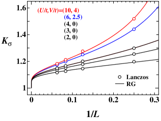
Figure 4: (Color online) TL liquid parameter $K_{\sigma}$ of finite size systems $L=4,8,12,16$ (open circles) for several choices of $(U/t,V/t)$.The solid lines denote the scaling trajectories of $K_{\sigma}(l)$ with $l=\ln L$.

The $T$ dependence of the $G_{4\sigma}(T)$ coupling can be obtained by using eq. (16), where we need the $T$ dependence of the spin velocity. The RG equation for the spin velocity has not been obtained without ambiguity, since the correction is not logarithmic and the scaling invariance is not retained. Thus we utilize the simple size dependence of the velocity to examine its $T$ dependence. The finite size scaling relation is expressed as

$$v_{\sigma}(L)=v_{\sigma}(\infty)+c_{1}/L+c_{2}/L^{2},$$ (24)

where $c_{1}$ and $c_{2}$ are numerical constants. In order to obtain the $T$ dependence of the spin velocity, we use eq. (24) by substituting $L=\mathrm{e}^{l}\simeq Ct/T$ with $C$ being an $O(1)$ numerical constant.

Appendix B Spin Susceptibility in One-Dimensional Hubbard Model

Figure 5: (Color online) $T$ dependence of the uniform spin susceptibility $\chi_{\sigma}$ in unit of $1/(ta)$ for the 1D Hubbard model, for several choices of $U/t$. The filled circle and the open circle represent the results by “Lanczos+Bosonization+RG” and those by “Bosonization+RG”, respectively (see text). These results are compared with QMC results (filled square for $L=64$ and filled triangle for $L=128$).

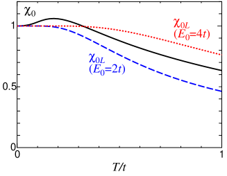
Figure 6: (Color online) $T$ dependence of the normalized uniform susceptibility $\chi_{0}(T)$ in the case of $\epsilon(K)=-2t\cos Ka$ (solid curve) and the susceptibility $\chi_{0L}(T)$ for $\epsilon(K)=v_{F}(pK-k_{F})$ with $|\epsilon(K)|<E_{0}/2$ (dashed curve for $E_{0}=2t$ and dotted one for $E_{0}=4t$).

In this section, we demonstrate the validity and the advantage of our combined analytical and numerical method by evaluating the uniform spin susceptibility of the 1D Hubbard model as a function of $T$. The present method (Lanczos+Bosonization+RG) is compared with the QMC method, as well as the conventional method based on the RG theory (Bosonization+RG). We summarize the results in Fig. 5, where the case for $U/t=2.0$ (a), 3.0 (b), and 4.0 (c) are shown. Both the “Lanczos+Bosonization+RG” method and the usual “Bosonization+RG” method can reproduce the QMC results qualitatively. Especially, the present method gives more accurate results compared with the usual method even in the strong interaction cases. We note that, the discrepancy between the present results and the QMC method is mainly due to the formula of the spin susceptibility, eq. (15). The formula (15) is based on the RPA formalism with renormalized parameters, which overestimates the absolute value.[30] It should be noted that the noninteracting susceptibility $\chi_{0}(T)$ is evaluated by using the cosine-band dispersion even in the “Bosonization+RG” method instead of the linearized dispersion, in order to see the importance of choice of the initial values of the RG equations. In the case of the linearized dispersion, the noninteracting susceptibility is written as

$$\chi_{0L}(T)=\tanh\frac{E_{0}}{4T},$$ (25)

where the energy dispersion is terminated as $-E_{0}/2<v_{F}(pK-k_{F})<E_{0}/2$ with $p=\pm$. This shows monotonic decrease with increasing $T$ and the comparison between the cosine-band dispersion and the linearized dispersion is shown in Fig. 6.

References

- [1] M. Imada, A. Fujimori, and Y. Tokura: Rev. Mod. Phys. 70 (1998) 1039.
- [2] H. Seo, C. Hotta, and H. Fukuyama: Chem. Rev. 104 (2004) 5005.
- [3] H. Seo, J. Merino, H. Yoshioka, and M. Ogata: J. Phys. Soc. Jpn. 75 (2006) 051009.
- [4] H. Yoshioka, M. Tsuchiizu, and Y. Suzumura: J. Phys. Soc. Jpn. 70 (2001) 762.
- [5] S. Ejima, F. Gebhard, and S. Nishimoto: Europhys. Lett. 70 (2005) 492.
- [6] C. S. Hellberg: J. Appl. Phys. 89 (2001) 6627.
- [7] J. Merino and R. H. McKenzie: Phys. Rev. Lett. 87 (2001) 237002.
- [8] R. Pietig, R. Bulla, and S. Blawid: Phys. Rev. Lett. 82 (1999) 4046; N. H. Tong, S. Q. Shen, and R. Bulla: Phys. Rev. B 70 (2004) 085118.
- [9] J. Merino, A. Greco, N. Drichko, and M. Dressel: Phys. Rev. Lett. 96 (2006) 216402.
- [10] K. Hanasaki and M. Imada: J. Phys. Soc. Jpn. 74 (2005) 2769.
- [11] Y. Tanaka: Dr. Thesis, Faculty of Science, University of Tokyo (2006).
- [12] H. Yoshioka, M. Tsuchiizu, and H. Seo: J. Phys. Soc. Jpn. 75 (2006) 063706.
- [13] H. Yoshioka, M. Tsuchiizu, and H. Seo: J. Phys. Soc. Jpn. 76 (2007) 103701.
- [14] H. Seo, Y. Motome, and T. Kato: J. Phys. Soc. Jpn. 76 (2007) 013707.
- [15] Y. Otsuka, H. Seo, Y. Motome, and T. Kato: J. Phys. Soc. Jpn. 77 (2008) 113705.
- [16] D. J. Scalapino, Y. Imry, and P. Pincus: Phys. Rev. B 11 (1975) 2042.
- [17] H. Seo and M. Ogata: Phys. Rev. B 64 (2001) 113103.
- [18] K. Sano and Y. Ōno: Phys. Rev. B 70 (2004) 155102.
- [19] H. J. Schulz: in Strongly Correlated Electronic Materials, ed. K. S. Bedell, Z. Wang, D. E. Meltzer, A. V. Balatsky, and E. Abraham (Addison-Wesley, Reading, 1994), p. 187.
- [20] T. Giamarchi: Physica B 230-232 (1997) 975.
- [21] J. L. Cardy: J. Phys. A: Math. Gen. 19 (1986) L1093.
- [22] M. Tsuchiizu, H. Yoshioka, and Y. Suzumura: J. Phys. Soc. Jpn. 70 (2001) 1460.
- [23] V. J. Emery: in Highly Conducting One Dimensional Solids, ed. J. Devreese, R. Evrard, and V. van Doren (Plenum, New York, 1979), p. 247.
- [24] In eq. (14) of ref. 12, is proproportional to the expectation value of . The ambiguity enters in the coefficient , of which its non-perturpative expression is unknown.
- [25] A. W. Sandvik and J. Kurkijärvi: Phys. Rev. B 43 (1991) 5950.
- [26] A. W. Sandvik: J. Phys. A 25 (1992) 3667.
- [27] A. W. Sandvik: Phys. Rev. B 59 (1999) R14157.
- [28] P. Sengupta, A. W. Sandvik, and D. K. Campbell: Phys. Rev. B 65 (2002) 155113.
- [29] H. Nlisse, C. Bourbonnais, H. Touchette, Y. M. Vilk, and A.-M. S. Tremblay: Eur. Phys. J. B 12 (1999) 351.
- [30] Y. Fuseya, M. Tsuchiizu, Y. Suzumura, and C. Bourbonnais: J. Phys. Soc. Jpn. 74 (2005) 3159.
- [31] T. Giamarchi: Phys. Rev. B 44 (1991) 2905.
- [32] T. Giamarchi: Phys. Rev. B 46 (1992) 342.
- [33] Y. Tanaka and M. Ogata: J. Phys. Soc. Jpn. 74 (2005) 3283.
- [34] C. Coulon, S. S. P. Parkin, and R. Laversanne: Phys. Rev. B 31 (1985) 3583.
- [35] F. Nad and P. Monceau: J. Phys. Soc. Jpn. 75 (2006) 051005.
- [36] T. Kakiuchi, Y. Wakabayashi, H. Sawa, T. Itou, and K. Kanoda: Phys. Rev. Lett. 98 (2007) 066402.
- [37] H. Seo and Y. Motome: Phys. Rev. Lett. 102 (2009) 196403.
- [38] K. Hiraki and K. Kanoda: Phys. Rev. B 54 (1996) R17276.
- [39] T. Itou, K. Kanoda, K. Murata, T. Matsumoto, K. Hiraki, and T. Takahashi: Phys. Rev. Lett. 93 (2004) 216408.
- [40] K. Hiraki and K. Kanoda: Phys. Rev. Lett. 80 (1998) 4737.
- [41] D. S. Chow, F. Zamborszky, B. Alavi, D. J. Tantillo, A. Baur, C. A. Merlic, and S. E. Brown: Phys. Rev. Lett. 85 (2000) 1698.
- [42] M. Fourmigué, E. W. Reinheimerab, K. R. Dunbar, P. Auban-Senzier, C. Pasquier, and C. Coulon: Dalton Trans. (2008) 4652.
- [43] K. Heuzé, M. Fourmigué, P. Batail, C. Coulon, R. Clérac, E. Canadell, P. Auban-Senzier, S. Ravy, and D. Jérome: Adv. Mater. 15 (2003) 1251.
- [44] P. Auban-Senzier, C. R. Pasquier, D. Jérome, S. Suh, S. E. Brown, C. Mézière, and P. Batail: Phys. Rev. Lett. 102 (2009) 257001.
- [45] B. Rothaemel, L. Forró, J. R. Cooper, J. S. Schilling, M. Weger, P. Bele, H. Brunner, D. Schweitzer, and H. J. Keller: Phys. Rev. B 34 (1986) 704.
- [46] H. Nishikawa, Y. Sato, K. Kikuchi, T. Kodama, I. Ikemoto, J. Yamada, H. Oshio, R. Kondo, and S. Kagoshima: Phys. Rev. B 72 (2005) 052510.
- [47] J. Ouyang, K. Yakushi, Y. Misaki, and K. Tanaka: Phys. Rev. B 63 (2001) 054301.
- [48] K. Yakushi, K. Yamamoto, M. Simonyan, J. Ouyang, C. Nakano, Y. Misaki, and K. Tanaka: Phys. Rev. B 66 (2002) 235102.
- [49] H. Mori, S. Tanaka, and T. Mori: Phys. Rev. B 57 (1998) 12023.
- [50] N. Tajima, M. Tamura, Y. Nishio, K. Kajita, and Y. Iye: J. Phys. Soc. Jpn. 69 (2000) 543.
- [51] S. Kimura, T. Maejima, H. Suzuki, R. Chiba, H. Mori, T. Kawamoto, T. Mori, H. Moriyama, Y. Nishio, and K. Kajita: Chem. Comm. (2004) 2454.
- [52] N. Morinaka, K. Takahashi, R. Chiba, F. Yoshikane, S. Niizeki, M. Tanaka, K. Yakushi, M. Koeda, M. Hedo, T. Fujiwara, Y. Uwatoko, Y. Nishio, K. Kajita, and H. Mori: Phys. Rev. B 80 (2009) 092508.
- [53] H. Yamada and Y. Ueda: J. Phys. Soc. Jpn. 68 (1999) 2735.
- [54] T. Yamauchi and Y. Ueda: Phys. Rev. B 77 (2008) 104529.
- [55] T. Giamarchi: Quantum Physics in One Dimension (Oxford University Press, Oxford, 2004).