NLO QCD corrections to $\mathbf{{\mathrm{t}}\bar{\mathrm{t}}{\mathrm{b}}\bar{\mathrm{b}}}$ production at the LHC

Abstract:

The next-to-leading order (NLO) QCD corrections to ${\mathrm{p}}{\mathrm{p}}\to{\mathrm{t}}\bar{\mathrm{t}}{\mathrm{b}}\bar{\mathrm{b}}$ at the LHC reveal that the scale choice adopted in previous lowest-order simulations underestimates the ${\mathrm{t}}\bar{\mathrm{t}}{\mathrm{b}}\bar{\mathrm{b}}$ cross section by a factor two. We discuss a new dynamical scale that stabilizes the perturbative predictions and describe the impact of the corrections on the shape of distributions. We also account for the techniques employed to compute the six-particle one-loop amplitudes with high CPU efficiency.

1 Introduction

The discovery of the Higgs boson and the measurement of its interactions with massive quarks and vector bosons represent a central goal of the Large Hadron Collider (LHC). In the mass range $114\,\mathrm{GeV}<M_{\mathrm{H}}\mathrel{\raisebox{-3.00003pt}{$\stackrel{{\scriptstyle\displaystyle<}}{{\sim}}$}}130\,\mathrm{GeV}$, associated ${\mathrm{t}}\bar{\mathrm{t}}{\mathrm{H}}$ production provides the opportunity to observe the Higgs boson in the ${\mathrm{H}}\to{\mathrm{b}}\bar{\mathrm{b}}$ decay channel and to measure the top-quark Yukawa coupling. However, the extraction of the ${\mathrm{t}}\bar{\mathrm{t}}{\mathrm{H}}({\mathrm{H}}\to{\mathrm{b}}\bar{\mathrm{b}})$ signal from its large QCD backgrounds, ${\mathrm{p}}{\mathrm{p}}\to{\mathrm{t}}\bar{\mathrm{t}}{\mathrm{b}}\bar{\mathrm{b}}$ and ${\mathrm{t}}\bar{\mathrm{t}}{\mathrm{j}}{\mathrm{j}}$, represents a serious challenge. The selection strategies elaborated by ATLAS and CMS [1, 2], which assume $30\,\mathrm{fb}^{-1}$ and $60\,\mathrm{fb}^{-1}$, respectively, anticipate a statistical significance around $2\sigma$ (ignoring systematic uncertainties) and a signal-to-background ratio as low as 1/10. This calls for better than 10% precision in the background description, a very demanding requirement both from the experimental and theoretical point of view. Very recently, a novel selection strategy based on highly boosted Higgs bosons has opened new and very promising perspectives [3]. This approach might increase the signal-to-background ratio beyond $1/3$.

The calculation of the NLO QCD corrections to the irreducible ${\mathrm{t}}\bar{\mathrm{t}}{\mathrm{b}}\bar{\mathrm{b}}$ background, first presented in  [4, 5] and subsequently confirmed in  [6], constitutes another important step towards the observability of ${\mathrm{t}}\bar{\mathrm{t}}{\mathrm{H}}({\mathrm{H}}\to{\mathrm{b}}\bar{\mathrm{b}})$ at the LHC. These NLO predictions are mandatory in order to reduce the huge scale uncertainty of the lowest-order (LO) ${\mathrm{t}}\bar{\mathrm{t}}{\mathrm{b}}\bar{\mathrm{b}}$ cross section, which can vary up to a factor four if the QCD scales are identified with different kinematic parameters [7]. Previous results for five-particle processes that feature a signature similar to ${\mathrm{t}}\bar{\mathrm{t}}{\mathrm{b}}\bar{\mathrm{b}}$ indicate that setting the renormalization and factorization scales equal to half the threshold energy, $\mu_{\mathrm{R,F}}=E_{\mathrm{thr}}/2$, is a reasonable scale choice. At this scale the NLO QCD corrections to ${\mathrm{p}}{\mathrm{p}}\to{\mathrm{t}}\bar{\mathrm{t}}{\mathrm{H}}$ ($K\simeq 1.2$) [8], ${\mathrm{p}}{\mathrm{p}}\to{\mathrm{t}}\bar{\mathrm{t}}{\mathrm{j}}$ ($K\simeq$1.1) [9], and ${\mathrm{p}}{\mathrm{p}}\to{\mathrm{t}}\bar{\mathrm{t}}{\mathrm{Z}}$ ($K\simeq 1.35$) [10], are fairly moderate. This motivated experimental groups to adopt the scale $\mu_{\mathrm{R,F}}=E_{\mathrm{thr}}/2=m_{\mathrm{t}}+m_{{\mathrm{b}}\bar{\mathrm{b}}}/2$ for the LO simulation of the ${\mathrm{t}}\bar{\mathrm{t}}{\mathrm{b}}\bar{\mathrm{b}}$ background [1]. However, at this scale the NLO corrections to ${\mathrm{p}}{\mathrm{p}}\to{\mathrm{t}}\bar{\mathrm{t}}{\mathrm{b}}\bar{\mathrm{b}}$ turn out to be unexpectedly large $(K\simeq 1.8)$ [5, 6]. As we argue, a reliable perturbative description of ${\mathrm{t}}\bar{\mathrm{t}}{\mathrm{b}}\bar{\mathrm{b}}$ production requires a different scale choice [11].

The calculation of the NLO corrections to ${\mathrm{p}}{\mathrm{p}}\to{\mathrm{t}}\bar{\mathrm{t}}{\mathrm{b}}\bar{\mathrm{b}}$ constitutes also an important technical benchmark. The description of many-particle processes at NLO plays an central role for the LHC physics programme, and the technical challenges raised by these calculations have triggered an impressive amount of conceptual and technical developments. Within the last few months, this progress has lead to the first NLO results for six-particle processes at the LHC, namely for ${\mathrm{p}}{\mathrm{p}}\to{\mathrm{t}}\bar{\mathrm{t}}{\mathrm{b}}\bar{\mathrm{b}}$ [5, 6], the leading- [12] and the full-colour contributions [13] to ${\mathrm{p}}{\mathrm{p}}\to{\mathrm{W}}{\mathrm{j}}{\mathrm{j}}{\mathrm{j}}$, and for the $q\bar{q}$ contribution to ${\mathrm{p}}{\mathrm{p}}\to{\mathrm{b}}\bar{\mathrm{b}}{\mathrm{b}}\bar{\mathrm{b}}$ [14].

To compute the virtual corrections to ${\mathrm{t}}\bar{\mathrm{t}}{\mathrm{b}}\bar{\mathrm{b}}$ production we employ explicit diagrammatic representations of the one-loop amplitudes and numerical reduction of tensor integrals [15, 16]. The factorization of colour matrices, the algebraic reduction of helicity structures, and the systematic recycling of a multitude of common subexpressions—both inside individual diagrams and in tensor integrals of different diagrams that share common sub-topologies—strongly mitigate the factorial complexity that is inherent in Feynman diagrams and lead to a remarkably high CPU efficiency. The real corrections are handled with the dipole subtraction method [17]. Our results have been confirmed with the HELAC-1LOOP implementation of the OPP method [18, 19, 20] within the statistical Monte Carlo error of 0.2% [6].

2 Description of the calculation

In NLO QCD, hadronic ${\mathrm{t}}\bar{\mathrm{t}}{\mathrm{b}}\bar{\mathrm{b}}$ production involves the $2\to 4$ partonic channels $q\bar{q}\to{\mathrm{t}}\bar{\mathrm{t}}{\mathrm{b}}\bar{\mathrm{b}}$ (7 trees and 188 loop diagrams) and ${\mathrm{g}}{\mathrm{g}}\to{\mathrm{t}}\bar{\mathrm{t}}{\mathrm{b}}\bar{\mathrm{b}}$ (36 trees and 1003 loop diagrams). The $2\to 5$ bremsstrahlung contributions comprise the crossing-symmetric channels $q\bar{q}\to{\mathrm{t}}\bar{\mathrm{t}}{\mathrm{b}}\bar{\mathrm{b}}{\mathrm{g}}$, $q{\mathrm{g}}\to{\mathrm{t}}\bar{\mathrm{t}}{\mathrm{b}}\bar{\mathrm{b}}q$, and ${\mathrm{g}}\bar{q}\to{\mathrm{t}}\bar{\mathrm{t}}{\mathrm{b}}\bar{\mathrm{b}}\bar{q}$ (64 diagrams each), and the partonic process ${\mathrm{g}}{\mathrm{g}}\to{\mathrm{t}}\bar{\mathrm{t}}{\mathrm{b}}\bar{\mathrm{b}}{\mathrm{g}}$ (341 diagrams). Each contribution has been worked out twice and independently, resulting in two completely independent computer codes. The treatment of the $q\bar{q}$- and gluon-induced reactions are described in  [4] and  [11], respectively. Here we mainly focus on the virtual corrections in the gg channel.

Feynman diagrams are generated with two independent version of FeynArts [21, 22] and handled with two in-house Mathematica programs that perform algebraic manipulations and generate Fortran77 code fully automatically. One of the two programs relies on FormCalc [23] for preliminary algebraic manipulations. The interference of the one-loop and LO matrix elements, summed over colours and helicities, is computed on a diagram-by-diagram basis,

$$\sum_{\mathrm{col}}\sum_{\mathrm{hel}}{\cal{M}}^{({\mbox{\scriptsize 1-loop}})}\left({\cal{M}}^{({\mathrm{LO}})}\right)^{*} = \sum_{\Gamma}\left[\sum_{\mathrm{col}}\sum_{\mathrm{hel}}{\cal{M}}^{(\Gamma)}\left({\cal{M}}^{({\mathrm{LO}})}\right)^{*}\right].$$ (1)

Individual loop diagrams $(\Gamma)$ are evaluated by separate numerical routines and summed explicitly. The cost related to the large number of diagrams is compensated by the possibility to perform colour sums very efficiently thanks to colour factorization [see (2)]. Individual (sub)diagrams consist of a single colour-stripped amplitude ${\cal A}^{(\Gamma)}$ multiplied by a simple colour structure, which is easily reduced to a compact colour basis ${\{\cal C}_{k}\}$. The LO amplitude is handled as a vector in colour space, and colour sums are encoded once and for all in a colour-interference matrix $I_{kl}$,

$${\cal{M}}^{(\Gamma)} = {\cal{A}}^{(\Gamma)}\left(\sum_{k}c_{k}^{(\Gamma)}{\cal C}_{k}\right),\qquad{\cal{M}}^{({\mathrm{LO}})}=\sum_{l}{\cal{M}}_{l}^{({\mathrm{LO}})}{\cal C}_{l},\qquad I_{kl}=\sum_{\mathrm{col}}{\cal C}_{k}{\cal C}^{*}_{l}.$$ (2)

These ingredients yield colour-summed results by means of a single evaluation of the colour-stripped amplitude ${\cal{A}}^{(\Gamma)}$ of each (sub)diagram. Tensor integrals with $N$ propagators and $P$ Lorentz indices are expressed in terms of totally symmetric covariant structures $\{g\dots gp\dots p\}^{\mu_{1}\dots\mu_{P}}_{j_{1}\dots j_{P}}$ involving external momenta $p_{1},\dots,p_{N-1}$ and $g^{\mu\nu}$ in $D=4-2\varepsilon$ dimensions  [16],

$$\frac{(2\pi\mu)^{4-D}}{{\mathrm{i}}\pi^{2}}\int{\mathrm{d}}^{D}q\,\frac{q^{\mu_{1}}\dots q^{\mu_{P}}}{\prod_{i=0}^{N-1}\left[(q+p_{i})^{2}-m_{i}^{2}+{\mathrm{i}}0\right]}=\sum_{j_{1},\dots,j_{P}=0}^{N-1}{T^{N}_{j_{1}\dots j_{P}}}\;{\{g\dots gp\dots p\}^{\mu_{1}\dots\mu_{P}}_{j_{1}\dots j_{P}}}.$$ (3)

The gg channel involves tensor integrals up to rank $P=4$. The coefficients $T^{N}_{j_{1},\dots,j_{P}}$ are related to scalar integrals by means of numerical algorithms that avoid instabilities from inverse Gram determinants and other spurious singularities [15, 16]. The tensor rank and the number of propagators of integrals with $N>4$ are simultaneously reduced without introducing inverse Gram determinants. Tensor integrals with $N=4,3$ are handled with the Passarino–Veltman algorithm as long as no small Gram determinant appears in the reduction. Otherwise, expansions about the limit of vanishing Gram determinants and possibly other kinematical determinants are applied [16]. The reduction is strongly boosted by a cache system that recycles tensor integrals among diagrams with common subtopologies. The ${\mathrm{g}}{\mathrm{g}}$ channel involves about 350 scalar integrals, which require $10\,$ms CPU time per phase-space point. The calculation of all scalar and tensor integrals with and without cache system takes $40\,$ms and $200\,$ms, respectively. Rational terms arising from ultraviolet (UV) poles of tensor integrals with $D$-dependent coefficients are automatically extracted by means of a catalogue of residues $R^{N}_{j_{1}\dots j_{P}}$,

$$f(D)T^{N}_{j_{1}\dots j_{P}} = f(D)\left(\hat{T}^{N}_{j_{1}\dots j_{P}}+\frac{R^{N}_{j_{1}\dots j_{P}}}{\epsilon_{\mathrm{UV}}}\right)=f(4)T^{N}_{j_{1}\dots j_{P}}-2f^{\prime}(4)R^{N}_{j_{1}\dots j_{P}}.$$ (4)

Rational terms resulting from infrared poles must be taken into account only in wave-function renormalization factors, since they cancel in truncated one-loop amplitudes [4].

The helicity-dependent parts of all diagrams are reduced to a common basis of so-called Standard Matrix Elements (SMEs) of the form

$${\hat{\cal{M}}}_{m}=Q_{m}^{\mu_{1}\mu_{2}\rho_{1}\dots\rho_{l}}\varepsilon_{\mu_{1}}(p_{1})\varepsilon_{\mu_{2}}(p_{2})\left[\bar{v}(p_{3})\gamma_{\rho_{1}}\dots\gamma_{\rho_{k}}u(p_{4})\right]\left[\bar{v}(p_{5})\gamma_{\rho_{k+1}}\dots\gamma_{\rho_{l}}u(p_{6})\right],\\$$

where $Q_{m}^{\mu_{1}\mu_{2}\rho_{1}\dots\rho_{l}}$ are combinations of metric tensors and external momenta. The colour-stripped part of each loop diagram [see (2)] yields a linear combination of SMEs and tensor integrals,

$${\cal{A}}^{(\Gamma)} = \sum_{m}{\cal F}^{(\Gamma)}_{m}{\hat{\cal{M}}}_{m},\qquad{\cal F}^{(\Gamma)}_{m}=\sum_{P}\sum_{j_{1},\ldots,j_{P}=0}^{N-1}{\cal K}^{(\Gamma)}_{m;j_{1}\dots j_{P}}{T^{N}_{j_{1}\dots j_{P}}}\;+\;\mbox{rational parts}.$$ (5)

The use of SMEs enables very efficient helicity summations. Helicity and colour sums are encoded in the interference of SMEs ${\hat{\cal{M}}}_{m}$ and colour structures ${\cal C}_{k}$ with the LO amplitude,

$$M_{km} = \sum_{\mathrm{col}}\sum_{\mathrm{hel}}{\hat{\cal{M}}}_{m}{\cal C}_{k}\left({\cal{M}}^{({\mathrm{LO}})}\right)^{*}=\sum_{l}I_{kl}\sum_{\mathrm{hel}}{\hat{\cal{M}}}_{m}\left({\cal{M}}^{({\mathrm{LO}})}_{l}\right)^{*}.$$ (6)

This matrix, which must be computed only once per phase-space point, links the colour/helicity-independent form factors ${\cal F}^{(\Gamma)}_{m}$ of each diagram to its colour/helicity-summed contribution

$$\sum_{\mathrm{col}}\sum_{\mathrm{hel}}{\cal{M}}^{(\Gamma)}\left({\cal{M}}^{({\mathrm{LO}})}\right)^{*} = \sum_{m}{\cal F}_{m}^{(\Gamma)}\left(\sum_{k}c_{k}^{(\Gamma)}M_{km}\right).$$ (7)

The SME-reduction starts with process-independent $D$-dimensional relations such as momentum conservation, Dirac algebra, transversality, and gauge-fixing conditions for the gluon-polarization vectors. Once rational terms are extracted, we further reduce SMEs with two alternative algorithms in four dimensions. The first algorithm splits each fermion chain into two contributions, $u(p_{i})=\sum_{\lambda=\pm}\omega_{\lambda}u(p_{i}),$ via insertion of chiral projectors $\omega_{\pm}=(1\pm\gamma^{5})/2$. This permits to employ various relations of type ${\gamma^{\mu}}{\gamma^{\alpha}\gamma^{\beta}}\omega_{\pm}\otimes{\gamma_{\mu}}={\gamma^{\mu}}\omega_{\pm}\otimes\left(\gamma_{\mu}\gamma^{\beta}\gamma^{\alpha}\omega_{\pm}+\gamma^{\alpha}\gamma^{\beta}\gamma_{\mu}\omega_{\mp}\right)$, which connect Dirac matrices of different fermion chains [4, 24]. In this way a rich variety of non-trivial identities are obtained that reduce the full amplitude to 502 SMEs [11]. Besides this procedure, which depends on process-specific aspects, we implemented a simple process-independent reduction based on a four-dimensional identity of type $\gamma^{\mu_{1}}\gamma^{\mu_{2}}\gamma^{\mu_{3}}\gamma^{\mu_{4}}\gamma^{\mu_{5}}=g^{\mu_{1}\mu_{2}}\gamma^{\mu_{3}}\gamma^{\mu_{4}}\gamma^{\mu_{5}}-g^{\mu_{1}\mu_{2}}g^{\mu_{3}\mu_{4}}\gamma^{\mu_{5}}+\mbox{perm.}$, which eliminates spinor chains with more than three Dirac matrices without introducing $\gamma_{5}$ [11]. This leads to 970 SMEs. In spite of the factor-two difference in the number of SMEs, we found that the numerical codes based on the two different reductions have the same—and remarkably high—CPU speed: about 180 ms per phase-space point. This unexpected result means that the obtained CPU performance, at least for this process, does not depend on process-dependent optimisations.

To handle the real corrections we employed the dipole subtraction method [17, 25]. The $2\to 5$ matrix elements were generated with Madgraph [26] and checked against analytic calculations and in-house code based on off-shell recursions. More details are given in  [11].

3 Predictions for the LHC

We present results for ${\mathrm{p}}{\mathrm{p}}\to{\mathrm{t}}\bar{\mathrm{t}}{\mathrm{b}}\bar{\mathrm{b}}+X$ at $\sqrt{s}=14\,\mathrm{TeV}$ for $m_{\mathrm{t}}=172.6\,\mathrm{GeV}$ and $m_{\mathrm{b}}=0$. Collinear final-state partons are recombined into jets with $\sqrt{\Delta\phi^{2}+\Delta y^{2}}>0.4$ using a $k_{{\mathrm{T}}}$-algorithm. We impose the cuts $p_{{\mathrm{T}},{\mathrm{b}}}>20\,\mathrm{GeV}$ and $|y_{\mathrm{b}}|<2.5$ on b jets and use the CTEQ6 set of PDFs with $N_{\mathrm{F}}=5$ active flavours and $\Lambda_{5}^{\overline{\mathrm{MS}}}=226\,\mathrm{MeV}$. Further details are given in  [11].

In all recent ATLAS studies of ${\mathrm{t}}\bar{\mathrm{t}}{\mathrm{H}}({\mathrm{H}}\to{\mathrm{b}}\bar{\mathrm{b}})$ [1] the signal and its ${\mathrm{t}}\bar{\mathrm{t}}{\mathrm{b}}\bar{\mathrm{b}}$ background are simulated by setting the renormalization and factorization scales equal to half the threshold energy, $E_{\mathrm{thr}}=2m_{\mathrm{t}}+m_{{\mathrm{b}}\bar{\mathrm{b}}}$. Being proportional to $\alpha^{4}_{\mathrm{s}}$, these LO predictions are extremely sensitive to the scale choice, and in  [5] we found that at $\mu_{\mathrm{R,F}}=E_{\mathrm{thr}}/2$ the NLO corrections to ${\mathrm{p}}{\mathrm{p}}\to{\mathrm{t}}\bar{\mathrm{t}}{\mathrm{b}}\bar{\mathrm{b}}$ are close to a factor of two. This enhancement is due to the fact that ${\mathrm{p}}{\mathrm{p}}\to{\mathrm{t}}\bar{\mathrm{t}}{\mathrm{b}}\bar{\mathrm{b}}$ is a multi-scale process involving various scales well below $E_{\mathrm{thr}}/2$. In particular, the cross section is saturated by b quarks with $p_{{\mathrm{T}},{\mathrm{b}}}\ll m_{\mathrm{t}}$ [11]. In order to avoid large logarithms we advocate the use of the dynamical scale

$$\mu^{2}_{0}=m_{\mathrm{t}}\sqrt{p_{{\mathrm{T}},{\mathrm{b}}}p_{{\mathrm{T}},\bar{\mathrm{b}}}},$$ (8)

which improves the perturbative convergence and minimises NLO effects in the shape of distributions [11].

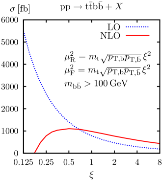
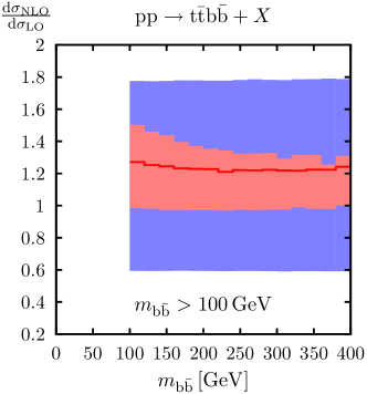
Figure 1: ${\mathrm{p}}{\mathrm{p}}\to{\mathrm{t}}\bar{\mathrm{t}}{\mathrm{b}}\bar{\mathrm{b}}+X$ cross section at the LHC for standard cuts and $m_{{\mathrm{b}}\bar{\mathrm{b}}}>100\,\mathrm{GeV}$: scale dependence of the LO and NLO cross section (left plot) and relative NLO corrections to the $m_{{\mathrm{b}}\bar{\mathrm{b}}}$ distribution (right plot).

In Fig. 1 we show results for the kinematic region $m_{{\mathrm{b}}\bar{\mathrm{b}}}>100\,\mathrm{GeV}$, which is relevant for ATLAS/CMS studies of ${\mathrm{t}}\bar{\mathrm{t}}{\mathrm{H}}({\mathrm{H}}\to{\mathrm{b}}\bar{\mathrm{b}})$. The left plot displays the dependence of the LO and NLO cross sections with respect to scale variations $\mu_{\mathrm{R}}=\mu_{\mathrm{F}}=\xi\mu_{0}$. At the central scale we obtain $\sigma_{\mathrm{LO}}=786.3(2)\,\mathrm{fb}$ and $\sigma_{\mathrm{NLO}}=978(3)\,\mathrm{fb}$. This NLO result is $2.18$ times larger as compared to the LO cross section based on the ATLAS scale choice [11]. The scale choice (8) reduces the $K$ factor to $1.24$, and the NLO (LO) uncertainty corresponding to factor-two scale variations amounts to 21% (78%). The improvement with respect to  [5] is evident also from the stability of the NLO curve in Fig. 1a. The right plot in Fig. 1 displays LO (blue) and NLO (red) scale-dependent predictions for the $m_{{\mathrm{b}}\bar{\mathrm{b}}}$ distribution. The results are normalized to the LO distribution at $\mu_{\mathrm{R,F}}=\mu_{0}$ and the bands correspond to factor-two scale variations. The NLO predictions perfectly fit within the LO band and exhibit little kinematic dependence. Inspecting various other distributions we found similarly small NLO corrections to their shapes.

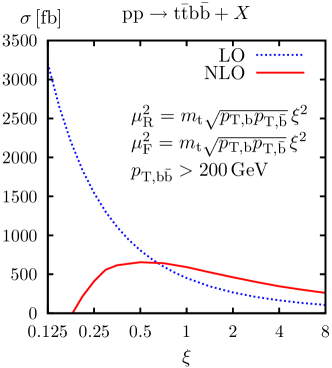
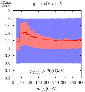
Figure 2: ${\mathrm{p}}{\mathrm{p}}\to{\mathrm{t}}\bar{\mathrm{t}}{\mathrm{b}}\bar{\mathrm{b}}+X$ cross section at the LHC for standard cuts and $p_{{\mathrm{T}},{\mathrm{b}}\bar{\mathrm{b}}}>200\,\mathrm{GeV}$: scale dependence of the LO and NLO cross section (left plot) and relative NLO corrections to the $m_{{\mathrm{b}}\bar{\mathrm{b}}}$ distribution (right plot).

In Fig. 2 we show similar plots for the kinematic region $p_{{\mathrm{T}},{\mathrm{b}}\bar{\mathrm{b}}}>200\,\mathrm{GeV}$, which permits to increase the separation between the Higgs signal and its ${\mathrm{t}}\bar{\mathrm{t}}{\mathrm{b}}\bar{\mathrm{b}}$ background [3]. At the central scale we obtain $\sigma_{\mathrm{LO}}=451.8(2)\,\mathrm{fb}$ and $\sigma_{\mathrm{NLO}}=592(4)\,\mathrm{fb}$. The $K$ factor (1.31), and the LO (79%) and NLO (22%) scale dependence behave similarly as for $m_{{\mathrm{b}}\bar{\mathrm{b}}}>100\,\mathrm{GeV}$. But in this case the NLO corrections are rather sensitive to $m_{{\mathrm{b}}\bar{\mathrm{b}}}$. In the physically interesting region of $m_{{\mathrm{b}}\bar{\mathrm{b}}}\sim 100\,\mathrm{GeV}$, the shape of the $m_{{\mathrm{b}}\bar{\mathrm{b}}}$ distribution is distorted by about 20%. This effect tends to mimic a Higgs signal and should be carefully taken into account in the ${\mathrm{t}}\bar{\mathrm{t}}{\mathrm{H}}({\mathrm{H}}\to{\mathrm{b}}\bar{\mathrm{b}})$ analysis.

4 Conclusions

The observation of the ${\mathrm{t}}\bar{\mathrm{t}}{\mathrm{H}}({\mathrm{H}}\to{\mathrm{b}}\bar{\mathrm{b}})$ signal and the direct measurement of the top-quark Yukawa coupling at the LHC require a very precise description of the ${\mathrm{p}}{\mathrm{p}}\to{\mathrm{t}}\bar{\mathrm{t}}{\mathrm{b}}\bar{\mathrm{b}}$ irreducible background. The NLO QCD corrections to ${\mathrm{t}}\bar{\mathrm{t}}{\mathrm{b}}\bar{\mathrm{b}}$ production reveal that the scale choice adopted in previous LO studies underestimates this cross section by a factor of two. We advocate the use of a dynamical scale that stabilizes the perturbative predictions reducing the $K$ factor to about $1.2$. In presence of standard cuts NLO effects feature small kinematic dependence. But in the regime of highly boosted Higgs bosons we observe significant distortions in the shape of distributions.

The calculation is based on process-independent algebraic techniques, which reduce loop diagrams to standard colour/helicity structures, and numerically stable tensor-reduction algorithms. The very high numerical stability and CPU efficiency of this approach are very encouraging in view of future NLO calculations for multi-particle processes.

References

- [1] G. Aad et al. [The ATLAS Collaboration], arXiv:0901.0512 [hep-ex].
- [2] G. L. Bayatian et al. [CMS Collaboration], J. Phys. G 34 (2007) 995.
- [3] T. Plehn, G. P. Salam and M. Spannowsky, arXiv:0910.5472 [hep-ph].
- [4] A. Bredenstein, A. Denner, S. Dittmaier and S. Pozzorini, JHEP 0808 (2008) 108.
- [5] A. Bredenstein, A. Denner, S. Dittmaier and S. Pozzorini, Phys. Rev. Lett. 103 (2009) 012002.
- [6] G. Bevilacqua, M. Czakon, C. G. Papadopoulos, R. Pittau and M. Worek, JHEP 0909 (2009) 109.
- [7] B. P. Kersevan and E. Richter-Was, Eur. Phys. J. C 25 (2002) 379; Comput. Phys. Commun. 149, 142 (2003).
-
[8]
W. Beenakker et al., Phys. Rev. Lett. 87 (2001) 201805;
Nucl. Phys. B 653 (2003) 151;
S. Dawson et al., Phys. Rev. D 67 (2003) 071503; Phys. Rev. D 68 (2003) 034022. - [9] S. Dittmaier, P. Uwer and S. Weinzierl, Phys. Rev. Lett. 98 (2007) 262002; Eur. Phys. J. C 59 (2009) 625.
- [10] A. Lazopoulos, T. McElmurry, K. Melnikov and F. Petriello, Phys. Lett. B 666 (2008) 62.
- [11] A. Bredenstein, A. Denner, S. Dittmaier and S. Pozzorini, arXiv:1001.4006 [hep-ph].
- [12] R. K. Ellis, K. Melnikov and G. Zanderighi, Phys. Rev. D 80, 094002 (2009).
- [13] C. F. Berger et al., Phys. Rev. D 80 (2009) 074036.
- [14] T. Binoth et al., arXiv:0910.4379 [hep-ph].
- [15] A. Denner and S. Dittmaier, Nucl. Phys. B 658 (2003) 175.
- [16] A. Denner and S. Dittmaier, Nucl. Phys. B 734 (2006) 62.
- [17] S. Catani, S. Dittmaier, M. H. Seymour and Z. Trócsányi, Nucl. Phys. B 627 (2002) 189.
- [18] G. Ossola, C. G. Papadopoulos and R. Pittau, Nucl. Phys. B 763, 147 (2007).
- [19] A. van Hameren, C. G. Papadopoulos and R. Pittau, JHEP 0909, 106 (2009).
- [20] M. Czakon, C. G. Papadopoulos and M. Worek, JHEP 0908 (2009) 085.
- [21] J. Küblbeck, M. Böhm and A. Denner, Comput. Phys. Commun. 60 (1990) 165.
- [22] T. Hahn, Comput. Phys. Commun. 140 (2001) 418.
- [23] T. Hahn and M. Pérez-Victoria, Comput. Phys. Commun. 118 (1999) 153.
- [24] A. Denner, S. Dittmaier, M. Roth and L. H. Wieders, Nucl. Phys. B 724 (2005) 247.
- [25] R. Frederix, T. Gehrmann and N. Greiner, JHEP 0809 (2008) 122.
- [26] J. Alwall et al., JHEP 0709 (2007) 028.