Level 1 on-ground telemetry handling in Planck LFI

Abstract

The Planck Low Frequency Instrument (LFI) will observe the Cosmic Microwave Background (CMB) by covering the frequency range 30-70 GHz in three bands. The primary instrument data source are the temperature samples acquired by the 22 radiometers mounted on the Planck focal plane. Such samples represent the scientific data of LFI. In addition, the LFI instrument generates the so called housekeeping data by sampling regularly the on-board sensors and registers. The housekeeping data provides information on the overall health status of the instrument and on the scientific data quality. The scientific and housekeeping data are collected on-board into telemetry packets compliant with the ESA Packet Telemetry standards. They represent the primary input to the first processing level of the LFI Data Processing Centre. In this work we show the software systems which build the LFI Level 1. A real-time assessment system, based on the ESA SCOS 2000 generic mission control system, has the main purpose of monitoring the housekeeping parameters of LFI and detect possible anomalies. A telemetry handler system processes the housekeeping and scientific telemetry of LFI, generating timelines for each acquisition chain and each housekeeping parameter. Such timelines represent the main input to the subsequent processing levels of the LFI DPC. A telemetry quick-look system allows the real-time visualization of the LFI scientific and housekeeping data, by also calculating quick statistical functions and fast Fourier transforms. The LFI Level 1 has been designed to support all the mission phases, from the instrument ground tests and calibration to the flight operations, and developed according to the ESA engineering standards.

1 Introduction

The Planck Science Ground Segment comprises the LFI and HFI Data Processing Centers (DPCs), the Mission Operations Control Centre (MOC) and the Planck Science Office (PSO). The LFI DPC is responsible of the data reduction and scientific processing of the LFI instrument, in order to extract the maximum amount of scientific information and provide the data quality necessary to achieve the objectives of the Planck mission (Tau04, ).

The LFI DPC activities have been decomposed into 4 levels, each one characterized by a subset of the data products generated during the Planck mission. In particular, the main input of the Level 1 is the raw telemetry of the instrument, compliant with the format specified by the ESA Packet Telemetry Standard (ESA88, ) and the Packet Utilization Standard (ESA02, ). Additional auxiliary input data is necessary to associate the telemetry data to a precise pointing of Planck and to correlate the on-board time (OBT) with the Universal Time (UTC) during flight operations. The Level 1 produces as output Time Ordered Information (TOI), i.e. time series, of each housekeeping and scientific parameter of LFI, together with additional diagnostic information necessary to monitor the health of the instrument and the data quality. The TOI are the primary input of the Level 2 and are also part of the final products of the LFI DPC versus the scientific community (after calibration and removal of systematic effects). They will also be used to create maps of the main astrophysical components.

This paper describes the software systems which are part of the Level 1 of Planck/LFI. A Real-Time Assessment system (RTA), based on the SCOS 2000 generic mission control system of ESA, provides monitoring tools to perform a routine analysis of the Spacecraft (S/C) and Payload (P/L) Housekeeping (HK) telemetry. A Telemetry Handling system (TMH) processes the raw telemetry packets by extracting the HK parameters and by uncompressing and decoding the LFI scientific samples (SCI); it produces homogeneous timelines for each HK and SCI parameter. A timeline contains for each sample, the OBT time, its raw and calibrated value together with additional flags on the data quality. A Telemetry Quick-Look system (TQL) provides interactive quick-look analysis tools, specific for the LFI instrument, to check both the SCI and HK telemetry and verify the normal behavior of the instrument.

The Level 1 software has been designed and developed in order to support all phases of the Planck/LFI mission, from the instrument ground tests, tuning and calibration to the integration tests and the flight operations. Priority has been given to the development of the core functionalities, common to all mission phases, and to maximizing code reuse. In this paper, we describe the software versions in use during the ground test campaigns (the so called Flight Models). The verification and validation of the Level 1 software, performed according to the ESA software engineering standard, has been described in (Fra09, ).

2 The LFI on-board data processing and telemetry structure

2.1 The on-board processing

In order to fully understand the operations performed by the Level 1 software, and in particular by the TMH/TQL systems, on the LFI scientific telemetry, we first provide an overview of the LFI acquisition chain and on-board processing.

The heart of the LFI instrument (Ber09, ) is an array of 22 radiometers fed by 11 corrugated feedhorns arranged in a circular pattern in the Planck focal plane. The receivers operate at three well separated bands: 30, 44 and 70 GHz. For each feedhorn, an ortho-mode transducer separates the two orthogonal polarization components. Each radiometer is a differential pseudo-correlation receiver (Men03, ) where the signals from the sky and from a reference load held at the constant temperature of 4 K are combined by a hybrid coupler, amplified in two independent amplifier chains, passed through a phase switch and separated out by another hybrid. The phase switch adds 0/180 degrees of phase lag to the signals and it is switched at 4 kHz synchronously in one of the two amplifier chains.

Hence, each radiometer provides two analog outputs, one for each amplifier chain. In a nominal configuration, each output yields a sequence of alternating $T_{load}$,$T_{sky}$ signals at the frequency of the phase switch. By changing the phase switches configuration, the output can be a sequence of either $T_{sky}$ or $T_{load}$ signals.

The conversion from analog to digital form of each radiometer output is performed by a 14 bits Analog-to-Digital Converter (ADC) in the Data Acquisition Electronics unit (DAE). The DAE transforms the signal in the range $[-2.5V,+2.5V]$: first it applies a tunable offset, $O_{\mathrm{DAE}}$, then it amplifies the signal with a tunable gain, $G_{\mathrm{DAE}}$, in order to make full use of the resolution of the ADC, and finally the signal is integrated. To eliminate phase switch raise transients, the integration takes into account a blanking time, i.e. a blind time in the integrator where data are not considered. The default value of the blanking time is 7.5 $\mu$s. Both the $O_{\mathrm{DAE}}$, the $G_{\mathrm{DAE}}$ and the blanking time are parameters set through the LFI on-board software. The equation applied to transform a given input signal $V_{\mathrm{in}}$ into an output $V_{\mathrm{out}}$ is

$$V_{\mathrm{out}}=G_{\mathrm{DAE}}(V_{\mathrm{in}}+O_{\mathrm{DAE}})+Z_{\mathrm{DAE}}$$ (1)

with $G_{\mathrm{DAE}}$ = 1, 2, 3, 4, 6, 8, 12, 16, 24, 48, $O_{\mathrm{DAE}}$ is one of 255 possible offset steps from +0 up to +2.5 V and where $Z_{\mathrm{DAE}}$ is a small offset introduced by the DAE when applying a selected gain. The values of $G_{\mathrm{DAE}}$ and $O_{\mathrm{DAE}}$ are set by sending, through specific telecommands, the DAE Gain Index (DGI) and the DAE Offset Index (DOI) associated to the desired values. A calibration table is needed for each offset step in order to best estimate how many volts have been removed.

The ADC quantizes the $V_{\mathrm{out}}$ uniformly in the range $-2.5\mathrm{V}\leq V_{\mathrm{adc}}\leq+2.5\mathrm{V}$, so that the quantization step is $q_{\mathrm{ADC}}=0.30518$ mV. The quantization formula is

$$P=\mathrm{round}\left[\frac{V_{\mathrm{out}}}{q_{\mathrm{ADC}}}\right],$$ (2)

and the output is stored as an unsigned integer of 16 bits.

The digitized scientific data is then processed by the Radiometer Electronics Box Assembly (REBA) which runs the LFI on-board software. The REBA is also in charge of processing the HK data (e.g. digital conversion of temperatures and voltages), keeping the OBT register synchronized with the S/C on-board clock, the generation of the LFI HK and SCI telemetry packets, the interpretation and execution of the telecommands sent from ground to the Spacecraft and in general the management of the entire instrument.

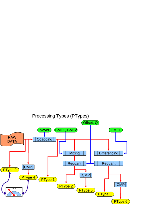
Figure 1: Schematic representation of the scientific on–board processing, processing parameters and processing types for the LFI. The diagram shows the sequence of operations leading to each processing type: coadding, mixing, requantization (Requant) and compression (CMP).

According to the ESA Standards, a source packet must include, in addition to the source data, a minimum of information needed by the ground system for the acquisition, storage and distribution of the source data to the end user. The source data is divided into several telemetry packets if it exceeds a prescribed maximum length.

Hence, the REBA processes data from each on-board data source in form of time series which are sampled at discrete times and split into packets to be sent to Earth. Since, in the Planck satellite, the telemetry packets of an entire operational day are stored into an on-board mass memory and then transmitted to the ground station during the Daily Tele-Communication Period (DTCP), the telemetry budget of the LFI instrument must not exceed the limit of 53.5 Kbps. To satisfy this limit, the REBA implements 7 acquisition modes (processing types) which reduce the scientific data rate by applying a number of processing steps. Fig. 1 illustrates the main steps of the on–board processing and the corresponding processing types (PTypes):

• PType 0: in this mode the REBA just packs the raw data of the selected channel without any processing.

• PType 1: consecutive sky or reference–load samples are coadded and stored as unsigned integers of 32 bits. The number of consecutive samples to be coadded is specified by the $\mathrm{N_{aver}}$ parameter.

• PType 2: in this mode, two main processing steps are applied. First, pairs of averaged sky and reference–load samples, respectively $\overline{S}_{sky}$ and $\overline{S}_{load}$, are mixed by applying two gain modulation factors, $\mathrm{GMF1}$ and $\mathrm{GMF2}$:

  $$P_{1} = \overline{S}_{sky}-\mathrm{GMF1}\cdot\overline{S}_{load}$$ (3)

  $$P_{2} = \overline{S}_{sky}-\mathrm{GMF2}\cdot\overline{S}_{load}$$ (4)

  The operations are performed as floating point operations. Then the values obtained are requantized converting them into 16-bit signed integers:

  $$Q_{i}=\mathrm{round}\left[\mathrm{SECOND\_QUANT}\left(P_{i}+\mathrm{OFFSET\_ADJUST}\right)\right]$$ (5)

• PType 3: with respect to PType 2, in this mode only a single gain modulation factor is used, $\mathrm{GMF1}$, obtaining:

  $$P = \overline{S}_{sky}-\mathrm{GMF1}\cdot\overline{S}_{load}$$ (6)

  and analogously to PType 2, the value is requantized obtaining 16-bit signed integer.

• With the processing types PType 4, PType 5, PType 6 the REBA performs a loss-less adaptive arithmetic compression of the data obtained respectively with the processing types PType 0, PType 2 and PType 3. The compressor takes couples of 16 bit numbers and stores them in the output string up to the complete filling of the data segment for the packet in process.

The set of REBA parameters – $\mathrm{N_{aver}}$, $\mathrm{GMF1}$, $\mathrm{GMF2}$, $\mathrm{SECOND\_QUANT}$ and $\mathrm{OFFSET\_ADJUST}$ – can be selected for each of the 44 LFI channels independently by sending dedicated telecommands. The calibration of the REBA parameters has been detailed in (Mar09, ).The REBA can acquire data from a channel in two modes at the same time. This capability is used to verify the effect of a certain processing type on the data quality. So, in nominal conditions, the LFI instrument will use the PType 5 for all its 44 detectors and every 15 minutes a single detector, in turn, will be processed also with PType 1 in order to periodically calibrate the gain modulation factors and the second quantization. The other processing types are mainly used for diagnostic, testing or contingency purposes.

The HK data processing is simpler since, basically, all the HK sources are polled at fixed times and analog sources are converted into digital form through an 8-bits linear ADC. The HK parameters are then grouped by: sub-system, information status (essential, nominal), purpose (monitoring, diagnostic) and sampling rate. Each group is tagged with a single OBT time and stored in the same telemetry packet.

In order to properly transform a data segment within a telemetry packet into a time series, each SCI and HK packet contains a time field associated to the first sample of the data segment. A clock internal to the REBA generates the sampling periods and the instrument OBT. Unavoidable drifts in the on–board clock lead to a loss of precise synchronization between the OBT and the universal time. For this reason the OBT is converted at ground to UTC (Universal Time Correlated).

2.1.1 Telemetry Packet Structure

Packets generated by the REBA follow the ESA Packet Telemetry Standard and Packet Telecommand Standard, the CCSDS Packet Telemetry recommendations (CCS95, ) and the ESA Packet Utilization Standard (PUS). Fig. 2 shows the general structure of the HK and SCI telemetry packets while Fig. 3 shows the general structure of a scientific data segment.

Packets are made of two headers of fixed length, a data segment of variable length and a 16 bits CRC field used to check the consistency of the packet. The specification of the Cyclic Redunndacy Code is provided in the ESA PUS, together with a reference implementation in C language.

All the packets have a primary header, carrying information about the type of packet (telecommand or telemetry) as well as a unique identifier of the on-board application process that has generated it (APID), a sequence counter and the total length of the packet. For telemetry packets, a secondary header of fixed length carries information about the type of service generating the packet (e.g. TC Verification, HK data reporting, Event reporting) and the on-board reference time of the packet.

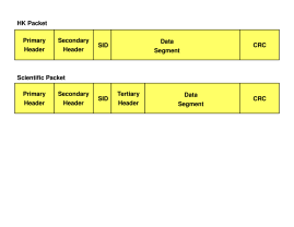
Figure 2: General structure of scientific and HK telemetry packets.

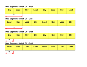
Figure 3: Content of the data segment for scientific packets of PType 0, 1, 2, 4, 5 after decompression and demixing (if needed). From top to bottom, packet with phase switch on, at even phase and odd phase, and with phase switch off, with even and odd phases. The double arrow with $T0$ denotes the samples with $t^{\mathrm{obt}}$ given by the packet timestamp. For PType $\neq 0$ and phase switch on, consecutive couples of samples have the same timestamp. When the phase switch is off, each sample has its hown $t^{\mathrm{obt}}$.

The sequence counter of the packet contains a sequential count (modulo 16384) of each packet by each source application process on the spacecraft. It allows the ground segment to detect possible gaps in the telemetry flow. The OBT is stored as a 48-bit field in CUC format, as specified in the PUS.

The aforementioned services are group of functionalities to be implemented on-board the satellite. Standard services are defined by the ESA PUS and are uniquely identified by a couplet of numbers (Type, Subtype). A service is invoked by a service request (telecommand source packet) which will result in the generation of zero or more service reports (telemetry source packet). Since a single service can generate several types of telemetry packets, with different structures, additional fields within the packet can be necessary to uniquely identify and properly parse a telemetry packet. Hence, in Planck most of the TM packets have a Structure ID field (SID). The set of fields (APID, Type, Subtype, SID) within a packet is used by the ground software to identify the data segment structure and extract the HK or the SCI samples.

Since the ESA PUS addresses only the utilization of telecommand packets and telemetry source packets for the purpose of remote monitoring and control of subsystems and payloads, an additional custom set of services has been defined by the PLANCK mission in order to handle the scientific telemetry.

2.1.2 Mapping SCI data into packets

After the SID, SCI telemetry packets contain a tertiary header of fixed length that includes the identifier of the detector that has generated the data, the phase switch status, the processing type applied to the data, the REBA parameters used for the processing, and the total number of samples stored in the packet (Gre08, ).

For the processing types PType 0, 1 and 4 the switching status defines whether the packet contains a sequence of interleaved sky and reference–load samples, or a sequence of only sky or only reference–load data. For PTypes 2 or 5 the switching status specifies the kind of sequence of samples produced by the demixing procedure applied at ground. For PTypes 3 and 6 it specifies which type of samples have been differentiated on-board.

The data segment of each SCI packet is filled up to the maximum length of 980 bytes. If data are compressed, the compressor stops the processing of new data when the maximum length is reached. The number of compressed samples is stored in the tertiary header in order to verify the consistency of the decompression. In case the acquisition is stopped, by sending a proper telecommand, the buffers of the REBA are flushed by storing the remaining data in new TM packets until the buffers are empty. In that case, packets much shorter than the maximum length may be generated.

At ground, packets have to be grouped according to their content and sorted by time, an action called registration and time unscrambling. Each packet contains all the relevant information to decode/decompress the data, register the data source and reconstruct the appropriated OBT of the packet. A packet contains consecutive samples produced for a given detector and generated according to a given processing type and for a given set of processing parameters. Any telecommand that changes one or more processing parameters for a given detector must be preceded by a telecommand stopping the acquisition.

In order to allow proper time reconstruction of all scientific samples, the OBT of each SCI packet corresponds to the time at which the first sample in the packet has been acquired. The time of the other samples within the packet is calculated based on the packet OBT and the channel frequency.

2.1.3 Mapping HK data into packets

The mapping of HK data into telemetry packets follows the rules provided in the ESA PUS. No compression is applied to the data segment and each field of such segment is either a parameter field containing a parameter value or a structured field containing several parameter fields. The PUS only indicates the parameter types of the parameter fields in the packet structures, such as boolean, enumerated, signed/unsigned integers with different octet sizes, real, character-string, absolute/relative time.

In general, in the HK packets the SID is followed by a sequence of values of housekeeping and diagnostic parameters that are sampled once per collection interval. The time of the samples correspond to the OBT of the packet.

In LFI, some of the HK packets are periodic, i.e. produced on a regular basis by the instrument, while others are produced only under particular conditions. The periodic HK packets report continuously the parameters of the instrument. They are classified in essential HK, fast HK and slow HK, according to their sampling rate. The essential telemetry is intended to be delivered to ground during the operations of the instrument when the satellite TM capability is limited by the use of the Low Gain Antenna. They are sent once every 32 seconds. The fast telemetry is sampled once per second. To avoid the generation of frequent short packets, some of the fast telemetry packets are super–commutated: the data segment is split into four sub-fields having the same structure (same parameters at the same relative offset). Each sub-field is sampled once per second and hence the whole packet is delivered every 4 seconds. Finally, the slow telemetry is generated once every 64 seconds.

The non-periodic telemetry includes packets which are generated only in response to a given telecommand (non-periodic packets) or packets, such as events and alarms, that can be automatically generated on-board when a certain condition arises.

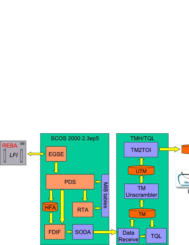
Figure 4: Level 1 architecture and data flow, showing the main components of each subsystem. The EGSE subsystem of SCOS receives the telemetry data from the REBA. The Packet Distribution System (PDS) forwards the telemetry packets to the Real-Time Assessment (RTA) displays, the History File Archive (HFA) and to the Flight Dynamic Interface (FDIF). Packets are properly parsed using the information stored in the Mission Information Base (MIB). The SODA task receives the real-time telemetry through the FDIF interface and forwards it to the TMH/TQL system. The off-line analysis of the TOI generated by the TMH, during the LFI calibration campaign, was performed using the LAMA software (Tom09, ).

3 The Level 1 software system overview

The LFI Level 1 software system is composed by three main subsystems (Fig. 4):

• a Real-time Assessment system. Based on the standard ESA SCOS-2000 system (Spacecraft Control & Operations System), it provides tools for monitoring the overall health of the instrument and detect possible anomalies (Scos03, ). The housekeeping data to be monitored include: temperature sensors output and stability, power consumption of individual units, cooling system parameters. Another set of tools is dedicated to the control of the instrument; they provide interfaces to select specific telecommands and set their parameter values, send the telecommands to the instrument control unit (the REBA) and receive TM reports on the execution status of each telecommand queued. Scripting capabilities are also provided in order to automatize and simplify the testing procedures during the ground test campaign.

• a TeleMetry Handler system. The TMH has been mainly developed by a team of the ISDC data centre in Geneva, by reusing part of the software modules they have developed for the INTEGRAL gamma-ray mission (Tur04, ). It receives the raw telemetry directly from the instrument, during the ground tests, or from the Mission Operation Centre (MOC), during Flight Operations. The TMH implements the so called Level 1 pipeline, a sequence of processing steps that starts with the reception of the raw telemetry and that terminates with the production of SCI and HK timelines, properly calibrated and converted into physical units.

• a Telemetry Quick-Look system. The TQL system provides a set of graphical tools to visualize the SCI and HK data, display them in real-time and calculates on-the-fly quick statistical functions and fast Fourier transforms. The same set of tools are also used to display the archived data. It provides several independent views of the data by supplying information on the source of the SCI telemetry flow at a given instant (radiometer and detector) and the processing type applied to a given detector data, highlighting telemetry gaps and producing XY-plots for the HK and SCI timelines, correlation plots and histograms.

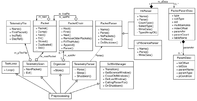
Figure 5: The TMU class diagram (in UML).

3.1 SCOS in the LFI LEVEL 1

SCOS 2000 is the generic mission control system software of ESA and runs under Sun/Solaris and Linux operating systems. It supports CCSDS telemetry and telecommand packet standards, and the ESA PUS. Telemetry and telecommand packets structure is kept in the SCOS Mission Information Base (MIB). This database is built for each mission, by providing a set of ASCII tables (MIB tables) that follow the format specified in the SCOS MIB Interface Control Document (ICD).

In addition to a set of configurable tasks that can be directly used to control and monitor an instrument, SCOS 2000 is also a reusable library of components with an object-oriented design and using standard design patterns. ESA SCOS 2000 is available under an open-source licensing scheme, giving the possibility to customize existing SCOS 2000 tasks or develop additional components.

SCOS 2000 is not able to process compressed scientific telemetry and the available graphical displays have still limited functionalities. For this reason SCOS 2000 is mainly used as an EGSE system (during the ground test campaign) and will also be used to monitor and visualize the LFI HK data during the flight operations. Since SCOS provides also TCP/IP and CORBA external interfaces, it is also used as a telemetry gateway between the instrument and the LFI TMH/TQL system.

SCOS 2000 is in charge of receiving the telemetry directly from the TM source, filling and maintaining a local database of raw packets, creating a list of stored packets, checking for missing, damaged or duplicated packets, displaying HK telemetry by converting raw data into physical data, generating and sending telecommands to the instrument through the testing environment or the MOC, checking OOL values and generating alarms to the operator.

The main task to configure the SCOS system for a particular instrument is the definition of the MIB database. It involves the mapping of all the instrument HK and telecommand packet structures into a subset of the MIB tables. For instance, the Packets Identification table (PID) includes, for each TM packet, the APID, Type, Subtype, and SID of that packet, representing its “primary key”. A monitoring Parameter Characteristics table (PCF) includes, for each HK parameter to be monitored, the parameter ID, its description and type, a reference to the calibration curve to be applied. A third table, the Parameter Location in Fixed packets table (PLF), associates a parameter of the PCF table to one or more packets of the PID table, by specifying its offset within the packet and eventually the number of occurrences (for super-commutated packets). An analogous procedure is followed to specify the telecommands structure. Additional information that can be provided in the MIB are the OOL values, that can be associated to validity criteria in order to distinguish among different test conditions (e.g. warm or cryogenic temperatures), conditional calibration curves, alphanumeric and graphic displays.

A dedicated software development was necessary to tailor specific SCOS 2000 tasks to the LFI ground segment, to allow the communication between SCOS 2000 and external systems. This tailoring has followed the SCOS release updates that were necessary during the mission preparation. For the tests involving only the LFI instrument, the EGSE system was based on SCOS 2.3e. In such version, the Telemetry Receiver (TMR), which is part of the SCOS 2000 simulators, has been modified in order to replay simulated LFI HK and SCI telemetry. To distribute the telemetry in real-time from SCOS to the TMH/TQL system, a task using the Flight Dynamic Interface of SCOS (FDIF) has been tailored in order to allow the TMH system to register as a SCOS client, set the list of packets to be distributed and receive a notification each time a live packet arrives (Fig. 4).

Starting from the Planck integration tests, the EGSE system adopted is the HPCCS. This system uses a new application protocol, called Packet Interface Protocol for EGSE (PIPE), to communicate with external equipments and software. With this new version, a new software has been developed, the LFIGatewy, acting as a telemetry gateway between the HPCCS main system operated by the Spacecraft instrument team and the client systems of the LFI instrument team (another HPCCS and the LFI TMH/TQL).

3.2 The Telemetry Handler System

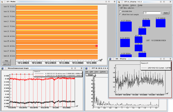
Figure 6: The TQL displays. The LFI modes display (top left) shows the processing type for all detectors of each horn. The status display window (top right) shows the status of all detectors of all horns, reporting if there is no data for a given detector or if normal scientific data or calibration data has been received at a given time. The mono-dimensional graph (bottom left) displays the load and sky data of one or more detectors as a function of time. On the bottom right two displays are shown: the fast Fourier transform of the sky signal for a single detector of feed-horn 18 (in background) and the HK display plotting a single LFI parameter as a function of time (in foreground).

The TMH system is the core of the Level 1 pipeline (Mor06, ). It receives real-time LFI telemetry from SCOS 2000 or from the LFIGateway and parses the content of each received TM packet to first discriminate between SCI and HK telemetry packets. SCI packets are then grouped according to the radiometer and detector source and to the applied processing type. For each group, the scientific data samples are uncompressed an decoded, the OBT of each sample is calculated based on the packet OBT and the detector frequency. At last, a calibration is applied to convert the raw sample value to Volts. The output is saved as a Time Ordered Information file in FITS format. HK telemetry packets are also grouped, according to the packet type. Their structure is recovered from the SCOS MIB files so that each HK parameter within the packet is properly extracted and converted into an engineering value according to its calibration curve. Again, for each parameter the output is a TOI. HK and SCI TOIs are then the input of the Level 2 of the LFI/DPC, where a more accurate calibration is performed. All these processing steps are divided into three main software components which form the pipeline.

The first component is the Data Receive module (Fig. 4). This component receives in real-time raw packets via a socket using the TCP/IP communication protocol. It runs continuously by reading incoming packets and storing the raw packets in a local TM archive, as FITS binary tables. Concurrently, it sends the raw packets also to the TQL system.

The second component is the TeleMetry Unsrcambler (TMU). It runs in near real-time and reads the raw packets from the TM archive. The TMU decodes the HK packets, groups them according to the APID, Type, Subtype and SID values, extracts the raw parameters values and saves them in an intermediate Unscrambled TeleMetry archive (UTM) as FITS files. For the SCI packets, it parses the information available in the tertiary header, groups and sorts the packets, and stores them in the UTM archive. At this level, the scientific samples are not yet decoded. In the UTM archive, each FITS file created covers a chunk of one hour in order to avoid too big files.

A simplified class diagram of the TMU is shown in Fig. 5. The main class, which executes the TMU event loop, is the Preprocessing class (Mor04, ). It inherits from five classes, each one implementing a subset of the Preprocessing tasks. The TaskLoop class implements the main Loop, by driving the activity of all the other components. The TelemetryScan class represents the Preprocessing input; it controls the access to the TM archive by providing a method, NextPacket(), which returns the subsequent telemetry packet available in the FITS archive. The Organizer class stores the incoming packets into packet chains (represented by the PacketChain class), using a distinct chain for each APID and sorting the packets by their sequence counter. Data are then reorganized into time slices named Science Windows. The ScWinManager class has the task of detecting a new science window depending on a particular criteria (e.g. pointing, slew, OBT interval) and the information included in specific packets. For LFI, the science windows are based on preconfigured OBT intervals. The TelemetryParser class processes each chain of telemetry packets by selecting the appropriate packet parser: the LFIScienceParser to decode SCI packets, or the HkParser to extract the parameters from the HK packets.

The last component of the TMH is the TM2TOI application. This component reads the UTM archive and produces the final product which is the Time Ordered Information(TOI) archive in FITS format. TM2TOI gathers the data of the same type, i.e. SCI data from the same detector and with the same processing or HK data from the same packet type, it retrieves the sky and load data (for science) and stores them in the TOI archive. For housekeeping data, TM2TOI produces one FITS file for each housekeeping parameter and applies calibration curves if necessary. TOI data are also stored by chunks of one hour and can be directly used for data analysis.

Each TOI includes time information in OBT format and converted into seconds. Science data are stored as sky and load samples. HK data are stored as raw samples with the corresponding converted values. A quality flag is also provided assuring the quality of the data.

3.3 The Telemetry Quick-Look

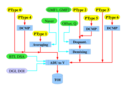
Figure 7: Schematic representation of the L1 processing for the various processing parameters and processing types for the LFI. $\mathrm{N_{aver}}$, $\mathrm{GMF1}$, $\mathrm{GMF2}$, $\mathrm{OFFSET\_ADJUST}$ (abbreviated with Offset), $\mathrm{SECOND\_QUANT}$ (abbreviated with Q), BTI and DSA are recovered from the tertiary header of each packet, DGI and DOI are recovered from the HK telemetry.

The scope of the TQL sub-system is to perform simple analysis of the data and display them together with the raw data in real-time. It is a progression of the display tools used for the INTEGRAL mission. Three displays are sufficient during the tests of the LFI instrument to verify the performance and to control the stability of the instrument. First the science data display, which can display any combination of the 44 scientific output streams. Second a mode display to verify the processing mode of each detector and finally graphs to display the housekeeping (HK) data in three different views: as a correlation plot of one HK parameter against several others, as a histogram plot, and, third, as a plot of any combination of HK parameters as a function of time. All displays can be operated in two modes. Either in real-time, to display the accumulated data during a ground test, or in playback mode, to display archived data. A subset of the TQL displays is shown in Fig. 6.

A toolkit is part of the scientific display to perform simple functions on the data. These functions are coded as ROOT macros , which can be interpreted in real-time by the program. For instance, the function displaying the fast Fourier transform of a given scientific channel is coded as a ROOT macro (see the FFT display in Fig. 6): it uses the fft function and the scientific samples exposed by the toolkit. Additional macros calculate quick statistics (mean, variance, skewness, kurtosis) of the displayed signal, or estimate the gain modulation factors on-the-fly, using the received sky and load samples. Each macro can be modified by the TQL user and new macros can be defined and loaded at run-time with the scientific display.

The ROOT framework is used as base library for all displays (Roh04, ). The ROOT CINT interpreter, part of every program, linked with the ROOT library, is used to interpret the toolkit macros. The capability of ROOT to store every object in a file is used to store the configuration of the displays for later use.

4 The Level 1 scientific data processing

When creating the TOIs, the Level 1 pipeline has to recover most accurately the values of the original (averaged) sky and load samples acquired on-board. The operations of each processing step performed by the TMH are illustrated in Fig. 7. Data acquired with PTypes 4, 5 and 6 first is uncompressed. The loss-less compression applied on-board is simply inverted and the number of samples obtained is checked with the value stored in the tertiary header.

Conversion to physical units

The digitized data, processed by the REBA, are not in physical units but in ADU (Analog to Digital Unit). Conversion of $\overline{S}_{sky}$ and $\overline{S}_{load}$ in Volt requires the Data Source Address ($\mathrm{DSA}$), indicating the radiometer and detector from which the data are generated, the blanking time (indicized by the Blancking Time Index, $\mathrm{BTI}$), the $\mathrm{DGI}$ and the $\mathrm{DOI}$. These values are recovered from the packet tertiary header. Hence, the value in Volt is obtained as:

$$\overline{V}_{i}=\frac{\overline{S}_{i}-Z_{\mathrm{DAE}}}{G_{\mathrm{DAE}}}-O_{\mathrm{DAE}}$$ (7)

This conversion is the only processing required by PTypes 0 and 3 and it is the last step in the processing of all the other processing types.

Dequantization and demixing

PType 2 and 5 data has to be dequantized by

$$P_{i}=\frac{Q_{i}}{\mathrm{SECOND\_QUANT}}-\mathrm{OFFSET\_ADJUST};$$ (8)

and then demixed to obtain $\overline{S}_{sky}$ and $\overline{S}_{load}$

$$\overline{S}_{sky} = \frac{\mathrm{GMF2}\cdot P_{1}-\mathrm{GMF1}\cdot P_{2}}{\mathrm{GMF2}-\mathrm{GMF1}};$$ (9)

$$\overline{S}_{load} = \frac{P_{2}-P_{1}}{\mathrm{GMF2}-\mathrm{GMF1}};$$ (10)

Averaging

Since PType 1 data is just coadded on-board, the division by $\mathrm{N_{aver}}$ is performed by the Level 1 software.

OBT reconstruction

The OBT reconstruction for scientific data has to take into account the phase switch status. If the phase switch is off, it means that the packet contains consecutive values of either sky or reference–load samples. In this case, denoting with $i_{\mathrm{smp}}\geq 0$ the sample index within the packet, we have that:

$$t^{\mathrm{obt}}_{i_{\mathrm{smp}}}=t^{\mathrm{obt}}_{0}+i_{\mathrm{smp}}\frac{N_{\mathrm{aver}}}{f_{\mathrm{sampling}}},$$ (11)

with $t^{\mathrm{obt}}_{0}$ the time stamp of the packet and $i_{\mathrm{smp}}=0$ denoting the first sample in the packet.

If the switching status is on, either consecutive pairs of (sky, reference–load) samples or (reference–load, sky) samples are stored in the packets. Hence, consecutive couples of samples have the same time stamp and

$$t^{\mathrm{obt}}_{i_{\mathrm{smp}}}=t^{\mathrm{obt}}_{0}+2\;{\mathrm{trunc}}\left[\frac{i_{\mathrm{smp}}}{2}\right]\frac{N_{\mathrm{aver}}}{f_{\mathrm{sampling}}}.$$ (12)

5 Conclusions

The LFI Level 1 software systems are successfully in use since five years to support the LFI instrument and calibration tests and the Planck integration and validation tests. Their design, development and testing has been performed according to the ESA software engineering standards. Their development has been based on already consolidated software: the ESA generic mission control system and the INTEGRAL ground segment of the ISDC. This paper has been focused on the software versions in use during the LFI calibration campaign and the Planck integration tests. The Operational Model (OM) of the Level 1 software, integrating the interfaces with the MOC that will be used during flight operations and a new I/O library, named Data Management Component (DMC), to store the TOIs and additional auxiliary data into a relational database system, has been presented in (Mor08, ) and will be the subject of an incoming paper.

- (1) J. A. Tauber, The Planck mission, Advances in Space Research 34 (2004) 491–496.
- (2) ESA Publications, Packet Telemetry Standard, Tech. Rep. PSS-04-106, ESA Procedures Standards and Specifications, 1988.
- (3) ESA Publications, Packet Utilization Standard (PUS), Tech. Rep. ECSS-E-70-41A, Issue 1, ESA Procedures Standards and Specifications, 2002.
- (4) M. Frailis, M. Maris, A. Zacchei, N. Morisset, R. Rohlfs, M. Meharga, P. Binko, M. Türler, S. Galeotta, F. Gasparo, E. Franceschi, R. C. Butler, O. D’Arcangelo, S. Fogliani, A. Gregorio, S. R. Lowe, G. Maggio, M. Malaspina, N. Mandolesi, P. Manzato, F. Pasian, F. Perrotta, M. Sandri, L. Terenzi, M. Tomasi, and A. Zonca, A systematic approach to the Planck LFI end-to-end test and its application to the DPC Level 1 pipeline, Journal of Instrumentation 12 (Dec., 2009) 12021–+.
- (5) M. Bersanelli, N. Mandolesi, R. C. Butler, A. Mennella, F. Villa, B. Aja, E. Artal, E. Artina, C. Baccigalupi, M. Balasini, G. Baldan, A. Banday, P. Bastia, P. Battaglia, T. Bernardino, E. Blackhurst, L. Boschini, C. Burigana, G. Cafagna, B. Cappellini, F. Cavaliere, F. Colombo, G. Crone, F. Cuttaia, O. D’Arcangelo, L. Danese, R. D. Davies, R. J. Davis, L. De Angelis, G. C. De Gasperis, L. De La Fuente, A. De Rosa, G. De Zotti, M. C. Falvella, F. Ferrari, R. Ferretti, L. Figini, S. Fogliani, C. Franceschet, E. Franceschi, T. Gaier, S. Garavaglia, F. Gomez, K. Gorski, A. Gregorio, P. Guzzi, J. M. Herreros, S. R. Hildebrandt, R. Hoyland, N. Hughes, M. Janssen, P. Jukkala, D. Kettle, V. H. Kilpia, M. Laaninen, P. M. Lapolla, C. R. Lawrence, J. P. Leahy, R. Leonardi, P. Leutenegger, S. Levin, P. B. Lilje, S. R. Lowe, D. L. P. M. Lubin, D. Maino, M. Malaspina, M. Maris, J. Marti-Canales, E. Martinez-Gonzalez, A. Mediavilla, P. Meinhold, M. Miccolis, G. Morgante, P. Natoli, R. Nesti, L. Pagan, C. Paine, B. Partridge, J. P. Pascual, F. Pasian, D. Pearson, M. Pecora, F. Perrotta, P. Platania, M. Pospieszalski, T. Poutanen, M. Prina, R. Rebolo, N. Roddis, J. A. Rubino-Martin, n. J. Salmon, M. Sandri, M. Seiffert, R. Silvestri, A. Simonetto, P. Sjoman, G. F. Smoot, C. Sozzi, L. Stringhetti, E. Taddei, J. Tauber, L. Terenzi, M. Tomasi, J. Tuovinen, L. Valenziano, J. Varis, N. Vittorio, L. A. Wade, A. Wilkinson, F. Winder, A. Zacchei, and A. Zonca, Planck pre-launch status: Design and description of the Low Frequency Instrument, ArXiv e-prints (Jan., 2010) [arXiv:1001.3321].
- (6) A. Mennella, M. Bersanelli, R. C. Butler, D. Maino, N. Mandolesi, G. Morgante, L. Valenziano, F. Villa, T. Gaier, M. Seiffert, S. Levin, C. Lawrence, P. Meinhold, P. Lubin, J. Tuovinen, J. Varis, T. Karttaavi, N. Hughes, P. Jukkala, P. Sjman, P. Kangaslahti, N. Roddis, D. Kettle, F. Winder, E. Blackhurst, R. Davis, A. Wilkinson, C. Castelli, B. Aja, E. Artal, L. de la Fuente, A. Mediavilla, J. P. Pascual, J. Gallegos, E. Martinez-Gonzalez, P. de Paco, and L. Pradell, Advanced pseudo-correlation radiometers for the Planck-LFI instrument, ArXiv Astrophysics e-prints (July, 2003) [astro-ph/].
- (7) M. Maris, M. Tomasi, S. Galeotta, M. Miccolis, S. Hildebrandt, M. Frailis, R. Rohlfs, N. Morisset, A. Zacchei, M. Bersanelli, P. Binko, C. Burigana, R. C. Butler, F. Cuttaia, H. Chulani, O. D’Arcangelo, S. Fogliani, E. Franceschi, F. Gasparo, F. Gomez, A. Gregorio, J. M. Herreros, R. Leonardi, P. Leutenegger, G. Maggio, D. Maino, M. Malaspina, N. Mandolesi, P. Manzato, M. Meharga, P. Meinhold, A. Mennella, F. Pasian, F. Perrotta, R. Rebolo, M. Türler, and A. Zonca, Optimization of Planck-LFI on-board data handling, Journal of Instrumentation 12 (Dec., 2009) 12018–+.
- (8) CCSDS, Packet Telemetry, Tech. Rep. 102.0-B-4, CCSDS Secretariat, 1995.
- (9) A. Gregorio, M. Miccolis, L. Stringhetti, A. Zacchei, R. C. Butler, and N. Mandolesi, Planck LFI User Manual, Tech. Rep. PL-LFI-PST-MA-001, University of Trieste, 2008.
- (10) M. Tomasi, A. Mennella, S. Galeotta, S. R. Lowe, L. Mendes, R. Leonardi, F. Villa, B. Cappellini, A. Gregorio, P. Meinhold, M. Sandri, F. Cuttaia, L. Terenzi, M. Maris, L. Valenziano, M. J. Salmon, M. Bersanelli, P. Binko, R. C. Butler, O. D’Arcangelo, S. Fogliani, M. Frailis, E. Franceschi, F. Gasparo, G. Maggio, D. Maino, M. Malaspina, N. Mandolesi, P. Manzato, M. Meharga, G. Morgante, N. Morisset, F. Pasian, F. Perrotta, R. Rohlfs, M. Türler, A. Zacchei, and A. Zonca, Off-line radiometric analysis of Planck-LFI data, Journal of Instrumentation 12 (Dec., 2009) 12020–+.
- (11) M. Jones, E. Gomez, F. Aldea, and H. Schäbe, SCOS-2000: Evaluating a Generic Mission Control System According To SPEC, in DASIA 2003, vol. 532 of ESA Special Publication, 2003.
- (12) M. Türler, R. Rohlfs, N. Morisset, M. T. Meharga, T. J.-L. Courvoisier, and R. Walter, From INTEGRAL to Planck: Geneva’s contribution to the LFI data processing, in Astronomical Data Analysis Software and Systems (ADASS) XIII (F. Ochsenbein, M. G. Allen, and D. Egret, eds.), vol. 314 of Astronomical Society of the Pacific Conference Series, pp. 440–+, July, 2004.
- (13) N. Morisset, R. Rohlfs, M. Türler, A. Mennella, M. Maris, S. Fogliani, X. Dupac, A. Zacchei, and D. Maino, Planck LFI Data Processing During Instrument Calibration Tests, in Astronomical Data Analysis Software and Systems XV (C. Gabriel, C. Arviset, D. Ponz, and S. Enrique, eds.), vol. 351 of Astronomical Society of the Pacific Conference Series, pp. 287–+, July, 2006.
- (14) N. Morisset, T. Contessi, M. T. Meharga, M. Beck, and R. Walter, Pre-processing the INTEGRAL telemetry, in Astronomical Data Analysis Software and Systems (ADASS) XIII (F. Ochsenbein, M. G. Allen, and D. Egret, eds.), vol. 314 of Astronomical Society of the Pacific Conference Series, pp. 388–+, July, 2004.
- (15) R. Rohlfs, The ROOT C++ Framework for Astronomy, in Astronomical Data Analysis Software and Systems (ADASS) XIII (F. Ochsenbein, M. G. Allen, and D. Egret, eds.), vol. 314 of Astronomical Society of the Pacific Conference Series, pp. 384–+, July, 2004.
- (16) N. Morisset, R. Rohlfs, M. Türler, M. Meharga, P. Binko, M. Beck, M. Frailis, A. Zacchei, and S. Galeotta, PLANCK LFI Level 1 Processing During Operations, in Astronomical Data Analysis Software and Systems XVII (R. W. Argyle, P. S. Bunclark, and J. R. Lewis, eds.), vol. 394 of Astronomical Society of the Pacific Conference Series, pp. 601–+, Aug., 2008.