Characterizing the Low-Mass Molecular Component in the Northern Small Magellanic Cloud

Abstract

We present here the first results from a high-resolution survey of the ¹²CO(J=1-0) emission across the northern part of the poorly-enriched Small Magellanic Cloud, made with the ATNF Mopra telescope. Three molecular complexes detected in the lower resolution NANTEN survey are mapped with a beam FWHM of $\sim$42^′′, to sensitivities of approximately 210 mK per 0.9 km s^-1 channel, resolving each complex into 4-7 small clouds of masses in the range of M${}_{vir}\sim$10^3-4M_⊙and with radii no larger than 16 pc.

The northern SMC CO clouds follow similar empirical relationships to the southern SMC population, yet they appear relatively under-luminous for their size, suggesting that the star-forming environment in the SMC is not homogeneous. Our data also suggests that the CO cloud population has little or no extended CO envelope on scales$\gtrsim$30 pc, further evidence that the weak CO component in the north SMC is being disassociated by penetrating UV radiation.

The new high-resolution data provide evidence for a variable correlation of the CO integrated brightness with integrated Hi and 160 $\mu$m emission; in particular CO is often, but not always, found coincident with peaks of 160 $\mu$m emission, verifying the need for matching-resolution 160 $\mu$m and Hi data for a complete assessment of the SMC H₂ mass.

1. Introduction

Molecular clouds are associated with the very earliest stages of star-formation and the environment external to the molecular cloud (e.g. enrichment levels, Interstellar medium (ISM) density variations, ambient magnetic and UV fields) must also play a significant role in the star-formation process. To understand the extent these and other parameters affect star-formation, we must examine the evolution of molecular clouds within a range of different environmental conditions.

The Magellanic Clouds are relatively metal poor; the LMC has a metallicity that is $\sim$30% of the solar value and the SMC about 10% of the solar value (e.g. Larsen et al., 2000). Furthermore, The molecular cloud population in the Magellanic Clouds are unique in the extra galactic molecular cloud ensemble; Bolatto et al. (2008) show that the molecular clouds in the south-west of the SMC are anomalously weak and under-luminous in comparison with other nearby extra galactic systems. At a distance of $\sim$60 kpc (e.g. Cioni et al., 2000, who report D${}_{SMC}\sim$ 63 kpc, however we use D${}_{SMC}\sim$ 60 kpc for consistency with existing liteurature), the SMC hosts a unique laboratory with an un-enriched ISM that is similar to that found in early-epoch and unevolved galaxies.

The molecular (i.e. H₂) component of galactic systems is most commonly estimated indirectly from observations of other tracers: e.g. from FIR or mm/sub-mm datasets and related to the CO fraction via empirically-derived relationships. Leroy et al. (2007) recently combined Hi and 160 $\mu$m observations of the SMC to estimate the molecular distribution and the $X_{SMC}$ factor (where the $X$ factor is an empirical conversion between CO and H₂; $X=N(H_{2})/W_{CO}$ cm^-2[K km s^-1]^-1). They find an $X_{SMC}$ factor that is broadly in agreement with those derived from virial mass estimates, if slightly higher. A higher $X_{SMC}$ factor implies that the actual mass of the CO clouds is greater equal to their measured virial mass, which may then require some magnetic support to prevent complete fragmentation. Leroy et al. (2007) (See also Bot et al. (2007) and Israel et al. (2003) - hereafter SKP-X, to indicate paper X of the SEST key project) go on to suggest that the H₂ component, which provides more effective self-shielding than does CO, resides in larger and weaker extended envelopes and is not as effectively traced by strong CO emission. In this scenario, the lower dust-to-gas ratio allows $UV$ radiation to penetrate further into the ISM and disassociate the outer CO layers to a level that is not detectable by current observations (See also Pak et al., 1998).

However Pineda et al. (2009) made a study of the $X$ factor as a function of a strongly varying UV field within the LMC (nearby to the bright star-forming region, 30 Doradus) and found that the value of $X$ and has a mean value of 3.9$\times$10²⁰cm^-2[K km s^-1]^-1; $\sim$2 $X_{Gal}$ but does not vary with the strength of the UV field. Given the apparent lower metallicity of the SMC relative to the LMC (e.g. Rolleston et al., 2003, 2002), we expect a higher $X_{SMC}$ factor and indeed, $X_{SMC}$ estimates are of the order of 10²¹ (e.g Leroy et al. 2007; Rubio et al. 1991; Israel et al. 1993-hereafter SKP-I,), with some exceptions where $X_{SMC}$ is found to be $\sim$10²⁰ (e.g. SKP-X).

Generally however, the existing measurements of the global molecular component of the SMC have been, by virtue of the weak emission, confined to very specific regions, often comprising a single pointing (e.g. Rubio et al., 1996, 2000; Israel et al., 1993, 2003, and references therein). In particular Rubio et al. (1993b; hereafter SKP-II), demonstrated the importance of high-resolution observations in resolving the molecular clouds and refining their basic morphological properties.

The NANTEN telescope has mapped the largest area of the SMC at any molecular transition (Mizuno et al., 2001; Blitz et al., 2007), covering the SMC bar, and parts of the eastern side. This 4 m telescope has a resolution of $\sim$2.6’ at the ¹²CO(J=1-0) line (sub-tending 44 pc at D$\sim$60 kpc), and so despite the excellent coverage, there remain some questions regarding the extent to which NANTEN can resolve molecular clouds in the SMC.

The existing targeted studies cannot form a resolved and comprehensive statistical study of the general molecular component in the SMC. It is therefore still impossible to completely understand the properties of the molecular clouds in the SMC as an ensemble, or to understand any large-scale systematic variations of the molecular cloud population throughout the SMC. It is with these issues in mind that we have undertaken to map the molecular component in the northern part of the SMC at high spatial resolution ($\sim$42$``$). This project forms the SMC branch of the molecular survey of the Magellanic System: ’Magellanic Mopra Assessment’ (MAGMA; Ott et al., 2008; Pineda et al., 2009).

In Section 2, we detail the observations and data reduction. In Section 3 we discuss the methods used to process and analyze the resulting data cubes. In Section 4 we briefly report on the results. Section 5 contains a discussion of the detected CO population in the context of the SMC ISM, and Section 6 summarizes our findings.

2. Observations and Data Reduction

Observation targets were selected from clouds in the north of the SMC that showed an integrated CO intensity of at least 0.2 K km s^-1 (as measured by NANTEN Mizuno et al., 2001). These clouds include those labeled NE-1 and NE-3; mapped at 8’.8 by Rubio et al. (1991) and we further extend the ensemble to include a previously unlabeled cloud, which we call NE-4. NE-4 is visible in maps by NANTEN (Mizuno et al., 2001) but has no specific reference in that work.

Observations were conducted during 2007, August and September with the the Mopra 22 m Telescope in Australia, and the UNSW-mops spectrometer. Observations were made using the ’zoom’ mode, where the 138 MHz-wide band is sampled with 4096 channels. Pointing accuracy was maintained by frequent (every 1.5 hours) observations of the SiO maser Upsilon Mensa, so that errors were typically less than 5″. Calibration and measurements of the T_sys were made from frequent ($\sim$15 minute interval) measurements of a hot load. The system temperature and data quality were monitored and calibrated using an in-horn diode calibrator.

Areas were scanned in overlapping 5$`$$\times$5$`$ regions. Each area was observed twice with a sampling rate of 2 seconds (equivalent to three integrations per $\sim$ 30” telescope beam-width), with orthogonal scanning directions to reduce scanning artifacts. Observations of ¹²CO(1-0) in Orion KL were made once each observing session to monitor telescope stability. The resulting peak flux measurements were found to be self-consistent within 10%, and also with observations made by the SEST telescope (see also Ladd et al., 2005). The data were baseline-corrected with a 0th order polynomial fit and doppler-corrected using the aips++ livedata package.

The cubes were formed using median weighting with the gridzilla package (beam-weighted gridding, and further smoothed with a radius-truncated Gaussian kernel, both with a FWHM of $\sim$35 arcseconds). Some of the spectra have a low-order and low-amplitude baseline variation present, which causes spurious detections in analysis software used later in this study. To remove this low-order baseline, the data cubes were differenced with a duplicate data cube, which was heavily smoothed in the frequency domain (width=26 km s^-1). As the expected linewidths of the CO emission were of the order of a few km s^-1(e.g. Rubio et al., 1996), this step does not significantly affect the measurement and results in a relatively minor adjustment to the mean power per channel (which was always less than the one-sigma noise level, as shown in Figure 1). Note also that any systematic or random errors arising from the baseline correction made here have not propagated through to the final brightness temperature estimates). Making this spectral smoothing-and-subtraction step improved the reliability of the cloud-searching algorithm by forcing the mean power outside channels containing emission to be approximately zero, and reduces false detections associated with a slowly-varying spectral baseline.

Figure 1.— Example of component that is removed from a sightline, following the spatial frequency-domain smoothing process described in the text. This spectrum is towards NE-1a (00:59:45 -71:44:40;J2000). The two horizontal lines indicate $\pm$1 $\sigma$ levels.

Finally, to improve sensitivity, the data cubes were binned to 0.9 km s^-1 and convolved with 30$``$ kernel, yielding an effective resolution of 42$``$ ($\sim$12 pc). The data cube was formed with a pixel size of 15$``$ ($\sim$4 pc). It should be noted that mops uses a large digital filter bank, rather than a traditional auto-correlator that operates in the Fourier domain. As a result, the frequency resolution is well approximated by the frequency channel spacing. Assuming an main-beam efficiency of 0.47 (e.g. Hughes et al., In prep.) at 115 GHz for the Mopra telescope, the resulting RMS level per channel is $\sim$ 210 mK (T_mb).

The maps and spectra for regions NE-1, NE-3 and NE-4 are shown in Figures 2, 3 and 4. These figures show the integrated intensity for pixels that were detected by cloudprops as containing emission only (See Section 3).

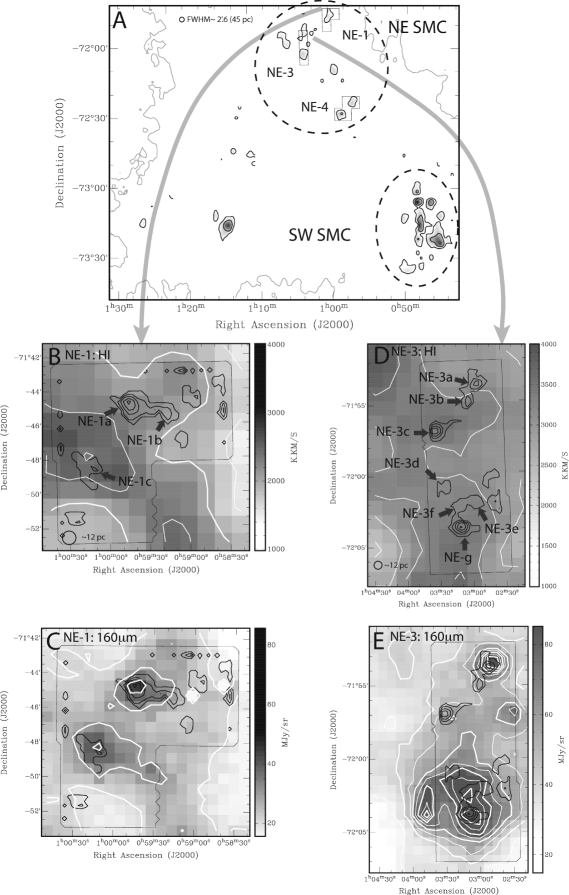
Figure 2.— Panel A: map of ¹²CO(1-0), from Mizuno et al. (2001) with boxes locating the areas which were observed by Mopra. Black contours are 0.3, 0.9 K km s^-1. NE-1 and NE-3 are shown in panels C and D, see Figure 4 for NE-4. The dotted ellipses clarify the terminology for ’Northeast’ and ’Southwest’ regions, as used in this report. The grey outer contour shows the 1$\times$10²¹ Hi integrated intensity level.
Panels B,C: Contours of Mopra CO observations (Black) made around NE-1, overlaid on integrated Hi (B) (Stanimirovic, 1999) and 160 $\mu$m(C) observations (Bolatto et al., 2007). CO contours show integrated brightness temperature levels 0.5+1 K km s^-1; White Hi and 160 $\mu$m contours are to aid visualization, and are at intervals of 400 K km s^-1 and 10 Mjy Str^-1 respectively.
Panels D,E: Contours of Mopra CO observations made around NE-3, overlaid on integrated Hi (D) and 160 $\mu$m (E) observations. CO contours show the 0.5+1 K km s^-1; Hi and 160 $\mu$m contours are to aid visualization, and are at intervals of 400 K km s^-1 and 10 Mjy Str^-1 respectively.

Figure 3.— Panels A: CO spectra towards peak positions of NE-1a and NE-1c, and Hi spectra towards NE-1a Bottom. The velocity centroids are marked with a vertical line. Note that the Hi profile shown in the bottom is measured towards NE-1a and approximately the same throughout the entire of NE-1
Panels B: CO spectra towards peak positions of NE-3a, NE-3c and NE-3g, and Hi spectra towards NE-3g Bottom. The CO velocity centroids are marked with a vertical line. As for Panel B, the Hi profile is measured only towards NE-3g, but is approximately the same throughout the entire of NE-3.

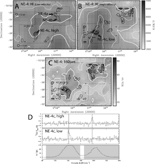
Figure 4.— Contours of Mopra CO observations made around NE-4, overlaid as black contours (0.5+1 K km s^-1) on integrated Hi (A, B) (Stanimirovic, 1999) and 160 $\mu$m (C) observations (Bolatto et al., 2007). The CO emission is broken into the high (Panel A) and low (panel B) velocity component and shown with the Hi also integrated over the high and low velocity ranges (shown as grayed regions in the top spectra of Panel D) . Both Hi and CO components are shown together in Panel C. White contours showing the Hi in intervals of 400 K km s^-1 (in Panels A,B), and in intervals of 10 Mjy str^-1 (in Panel C) to aid visualization.

3. Cloud Identification Procedure

The literature contains various methods of determining the radius of CO clouds detected in the SMC. Rubio et al. (1991) and Mizuno et al. (2001) choose to define the extent of the cloud based on the sensitivity of the data: pixels brighter than 3$\sigma$ in the integrated intensity maps are added and represent the area of the cloud. We attempt here an approach that is slightly less dependent on the quality of the observational data, where clusters of spectral lines containing emission are detected using a moment analysis by the (Rosolowsky & Leroy, 2006) analysis package cloudprops. We stress that cloudprops is used here only to objectively identify spectra containing emission within four adjacent velocity channels. cloudprops is not used for further analysis or interpretation and the observable parameters are measured from pixels that are identified by cloudprops as containing emission.

We apply cloudprops to identify regions containing signal greater than 1.5$\sigma$ (by setting the thresh parameter) over at least 4 spectral channels and spread over an area equal to or greater than the beam size ($\sim 42$$``$). We further examine cloud candidates by eye to eliminate spurious or marginal identifications. Typically, one or two putative ’clouds’ in each of the three regions were falsely identified by cloudprops, and were rejected.

We estimate the cloud radii, I_CO and L_CO by summing the area of pixels containing emission that are close to the same local integrated intensity maxima (i.e. we group together all pixels that are closest to the same local maxima). We use the common definitions of these parameters: Radius, R = $(Area/\pi)^{0.5}$, virial mass; where M_VIR= 190R$\Delta$V² (assuming a $1/r$ density profile throughout the cloud and where the velocity width ($\Delta$V) is measured at the position of maximum integrated brightness); and CO luminosity L_CO, estimated from the product of the mean integrated emission and cloud area. As the Mopra beam size and shape is not well understood and the SMC cloud radii are closely matched to the Mopra beam-size, we do not present the de-convolved radii of the clouds. We instead incorporate the de-convolved radius in the measurement errors by calculating the upper and lower errors separately: the lower error is equal to the de-convolved radius minus the measurement error of 2 pc. The errors reported for peak temperature are measurement errors only: we do not attempt to propagate the errors of the radius measurements and recalculate peak temperature measurement errors arising from beam dilution.

Line characteristics of spectra towards the position of peak integrated brightness (main beam brightness temperature, T_mb; velocity width, $\Delta$V; velocity centroid, V₀) are estimated by fitting a single-component Gaussian (using the Marquardt-Levenberg algorithm). Given the low Signal-to-noise (S/N) ratio of these CO spectra and their simple, single-component profiles, it is not appropriate or beneficial to seek to decompose the emission into more than one spectral component. The errors for observables obtained in this way are estimated as asymptotic errors using statistical algorithms developed by Landman et al. (1982).

It should be noted that the low S/N of these observations propagates to large errors in the fitted parameters, typically of around 50% or even greater. As such, the resulting best-fit Gaussian profiles were occasionally narrower than the instrumental resolution of the telescope (e.g. cloud NE-3d). Table 3 lists the cloud parameters : Peak T_mb, V₀, $\Delta$V, radius R, M_VIR, I_CO.

Table 1Northern SMC CO-cloud parameters

Cloud/complex	RA	Dec	Peak TMB	Vo	$\Delta$V	Radius	MVIR	LCO$\times$103
	(J2000)	J(2000)	[K]	[ km s-1]	[ km s-1]	[pc]	[$\times$103M⊙]	[K km s-1 pc2]
Complex NE-1
NE-1a	00:59:50	-71:44:40	1.2 $\pm$ 0.2	149.0 $\pm$ 0.2	3.4$\pm$0.6	16${}^{+2}_{-3}$	40${}^{+10}_{-10}$	1.5${}^{+0.5}_{-0.7}$
NE-1b	00:59:20	-71:45:30	0.8 $\pm$ 0.3	149.2 $\pm$ 0.3	2.1$\pm$0.8	9${}^{+2}_{-5}$	8${}^{+6}_{-7}$	0.3${}^{+0.2}_{-0.3}$
NE-1c	01:00:10	-71:48:40	0.9 $\pm$ 0.4	150.0 $\pm$ 0.3	2.0$\pm$0.7	13${}^{+2}_{-3}$	10${}^{+7}_{-8}$	0.6${}^{+0.2}_{-0.3}$
Complex NE-3/N76
NE-3a	01:02:50	-71:53:30	0.6 $\pm$ 0.1	169.2 $\pm$ 0.5	5$\pm$1	12${}^{+2}_{-3}$	60${}^{+30}_{-30}$	0.6${}^{+0.3}_{-0.4}$
NE-3b	01:03:00	-71:55:00	0.7 $\pm$ 0.2	171.9 $\pm$ 0.3	2.4$\pm$0.6	9${}^{+2}_{-4}$	11${}^{+6}_{-8}$	0.3${}^{+0.2}_{-0.3}$
NE-3c	01:03:30	-71:57:00	1.7 $\pm$ 0.2	175.4 $\pm$ 0.1	2.1$\pm$0.3	11${}^{+2}_{-4}$	10${}^{+3}_{-4}$	0.7${}^{+0.3}_{-0.5}$
NE-3d	01:03:20	-72:01:00	0.6 $\pm$ 0.2	168.6 $\pm$ 0.2	2.3$\pm$0.8	7${}^{+2}_{-7}$	8${}^{+6}_{-8}$	0.2${}^{+0.1}_{-0.2}$
NE-3e	01:03:00	-72:02:00	0.7 $\pm$ 0.2	168.3 $\pm$ 0.4	2.4$\pm$0.6	9${}^{+2}_{-4}$	11${}^{+6}_{-8}$	0.3${}^{+0.2}_{-0.3}$
NE-3f	01:03:10	-72:02:00	0.8 $\pm$ 0.2	168.1 $\pm$ 0.2	2.4$\pm$0.6	9${}^{+2}_{-4}$	11${}^{+6}_{-8}$	0.3${}^{+0.2}_{-0.3}$
NE-3g	01:03:10	-72:03:50	1.6 $\pm$ 0.3	168.6 $\pm$ 0.2	2.3$\pm$0.5	13${}^{+2}_{-3}$	14${}^{+6}_{-7}$	1.0${}^{+0.3}_{-0.5}$
Complex NE-4
NE-4ahi	00:57:00	-72:22:40	1.5 $\pm$ 0.3	153.9 $\pm$ 0.2	2.2$\pm$0.5	11${}^{+2}_{-4}$	11${}^{+5}_{-6}$	0.6${}^{+0.2}_{-0.4}$
NE-4bhi	00:56:50	-72:24:20	0.8 $\pm$ 0.2	154.1 $\pm$ 0.3	1.8$\pm$0.6	9${}^{+2}_{-5}$	6${}^{+4}_{-5}$	0.2${}^{+0.1}_{-0.2}$
NE-4chi	00:58:20	-72:28:10	1.3 $\pm$ 0.2	158.2 $\pm$ 0.2	2.3$\pm$0.5	15${}^{+2}_{-3}$	16${}^{+7}_{-8}$	0.9${}^{+0.3}_{-0.5}$
NE-4clow	00:58:40	-72:27:40	1.6 $\pm$ 0.3	122 $\pm$ 1	5$\pm$2	14${}^{+2}_{-3}$	70${}^{+60}_{-60}$	1.7${}^{+0.5}_{-0.9}$

To provide some assurance of the effectiveness of our data preparation and analysis technique, we apply it also to data of the south-west SMC, taken with the SEST telescope (Rubio et al., 1993a, hereafter, SKP-III). The analysis method we apply to the SEST dataset is almost identical to that used on the data presented here, with the exception of the smoothing-and-subtraction baseline correction step. This step was omitted primarily because the frequency-switching mode employed for the SEST observations generates a ”negative” spectral artifact nearby to the real emission spectrum, and also because insufficient line-free channels exist to create a usable smoothing function (as the emission line occurs near the edge of the band). Instead, we have removed a second-order baseline, interpolated from line-free channels across velocities channels where emission occurs.

We provide the results of this comparison in Table 2 and show that our method produces values that are consistent to within approximately 10% with the reported in SKP-III. Note that errors are not quoted in SKP-II and SKP-III, however the RMS for the SKP observations is cited as 200 mK, and later papers in that series cite T_mb accuracies of 15-20%.

Table 2Confirmation of cloud analysis algorithm

Cloud/Object	This paper	SKP-II, SKP-IIIa
LIRS36
Tmb [K]	2.4$\pm$0.1	2.37
$\Delta$V [K km s-1]	3.1$\pm$0.1	3.1
R [pc]	16.3$\pm$0.2	18.6
LCO[$\times$ 103 K km s-1 pc2]	2.0$\pm$0.5	2.8
LIRS49
Tmb [K]	1.6$\pm$0.1	1.88
$\Delta$V [K km s-1]	4.8$\pm$0.1	4.8
R [pc]	17.3$\pm$0.2	18.6
LCO[$\times$103 K km s-1 pc2]	6$\pm$1	6.41
SMCB1
Tmb [K]	1.4$\pm$0.1	1.38
$\Delta$V [K km s-1]	2.75$\pm$0.1	2.88
R [pc]	15.2$\pm$0.2	13.8
LCO[$\times$103 K km s-1 pc2]	1.3$\pm$0.4	1.21
N88
s Tmb [K]	0.79$\pm$0.1	0.77
$\Delta$V [K km s-1]	1.63$\pm$0.2	1.6
R [pc]	Unresolved.	Unresolved.
LCO[$\times$103 K km s-1pc2]	0.5$\pm$0.2	0.54

4. Properties of CO clouds in the SMC

Table 3 shows that the detected and most massive clouds in the northern SMC are relatively small, with virial masses in the 10^3-4M_⊙ range. This is at the extreme low end of an extra-galactic sample examined by Bolatto et al. (2008), where the virial masses of the extra-galactic molecular cloud ensemble exist over a range of $\sim$10^4-6M_⊙. We see then that the molecular cloud population in the northern SMC can be regarded as an extreme population relative to the south-west SMC, and more so in the extra-galactic context.

Figures 2, 3 and 4 show the relative distributions and ¹²CO(J=1-0) emission spectra of the three regions NE-1, NE-3 and NE-4. Also shown are the velocity-integrated I_CO maps overlaid on 160 $\mu$m and Hi data, as tracers of the big-grain (BG) dust abundance and temperature, and the ubiquitous ISM, respectively. Note that the Hi maps are of much poorer resolution ($\sim$98”) than the CO dataset and are used here to aid a contextual discussion of the relationships between Hi, CO and 160 $\mu$m tracers. The 160 $\mu$m  data is obtained directly from the S³MC archive (Bolatto et al., 2007) and have not been rigorously processed to remove, for example, the weak (but very complicated) contribution from foreground cirrus (See Leroy et al., 2007).

4.1. NE-1

We see in Figure 2 (Panels B and C) the spatial relationship of NE-1 with Hi and 160 $\mu$m respectively. The CO emission from this region is relatively weak, with a peak T_mb of barely over 1 K. The detected CO clouds are spatially coincident with the strongest sources of 160 $\mu$m emission in this region (Figure 2B), although there are some significant departures from a perfect correlation, most likely due to varying dust temperature and/or small-scale fluctuations in Hi column density that is not obvious from Figure 2C. Even so, and bearing in mind that the spatial resolution of the Hi observations is 98”; approximately three times that of the CO observations, Figure 2C shows the Hi integrated brightness varies only very slowly across the region with little evidence of any significant variations in intensity towards the CO sources.

We estimate the virial masses of the clouds (NE-1a, NE-1b and NE-1c) to be 4.0$\pm$1$\times$10⁴M_⊙, 8${}^{+6}_{-7}\times$10³M_⊙ and 10${}^{+7}_{-8}\times$10³M_⊙. Summed together, the mass of this complex measured by Mopra is approximately a factor of 50 below the virial mass estimated by Rubio et al. (1991). The combination of a lower resolved velocity dispersion (by a factor of $\sim$3) and lower radius (by a factor of $\sim$6) will account for the disagreements in estimated virial masses, however we explore the wider-scales of this complex further in Section 5.2.

The emission profiles associated with NE-1a and NE-1c are shown in Figure 3 (Panels A,B) and these observations have enabled the velocity components of the emission regions to be separated into much narrower profiles than was previously known. We see that the CO peaks generally coincide with Hi peaks, although not always at exactly the peak velocity.

4.2. NE-3

The CO emission from this region is shown overlaid on Hi integrated intensity and on 160 $\mu$m brightness in Figure 2 (Panels D,E respectively). The Figures show a slightly larger area than was mapped by Mopra to include the full extent of an apparently coherent 160 $\mu$m emission region. We resolve up to seven peaks of emission distributed throughout this region.

We find a total virial mass of 1.25${}^{+6.3}_{-7.3}\times$10⁵M_⊙; a factor of $\sim$100 less than that reported by Rubio et al. (1991). The difference in measured velocity widths and radii cannot account for the difference in the estimated virial masses, however, there appears to be some differences in the CO maps from Mizuno et al. (2001) and Rubio et al. (1991). After allowing for different beam sizes we find that the morphology of the NANTEN results are more consistent with the high resolution results presented here. We note that the NANTEN maps show additional CO clouds that seem confused or absent in the Rubio et al. (1991) study, and are approximately 10’ east of the area mapped with Mopra for the present study. We present a study of the larger-scale distribution of CO in the context of the NANTEN dataset in Section 5.2.

The distribution of the 160 $\mu$m emission associated with NE-3 again shows a generally good association of the peak 160 $\mu$m and CO (Figure 2E), and there are again some notable deviations from a good correlation. The Hi data (Figure 2D) shows a rather slowly-varying and uncorrelated distribution but are not of sufficient resolution to obtain a good estimate of the relationship of CO and H₂ on these scales observed with Mopra.

4.3. NE-4

The measured CO emission from NE-4 is shown in the top of Figure 4 as contours overlaid on Hi integrated over 85$<$V${}_{LSR}<$140 (Panel A) and 145$<$V${}_{LSR}<$200 (Panel B). All CO integrated over the line of sight is shown overlaid on 160 $\mu$m emission on Panel C (Bolatto et al., 2007).

Studies by Mizuno et al. (2001) resolve this complex into two clouds, although this work did not discuss this region in detail. We show here in Figure 4 that this region is now resolved further into four clouds, including a pair that shows evidence for easily-separable high and low velocity components, as shown in Figure 4D.

Panel D of Figure 4 shows that the CO emission peaks correspond closely, although not exactly in velocity to peaks of Hi. This suggests that the molecular and neutral components are to some extent, co-moving with the Hi. The projected spatial separation of the high and low velocity components of the two CO clouds is $\sim$30 pc. The fact that two separate regions are detected in close proximity may be evidence for a recent energetic event which has bifurcated a formed molecular cloud, however we will defer a more dedicated analysis of the velocity structure of the ISM at this location to a later paper.

The distribution of the 160 $\mu$m emission shown in Figure 4C, shows local maxima approximately spatially coincident with the CO emission, however once again, the resolution of the Hi data (Figure 4C) is too poor to permit a reliable estimate of the correlation of H₂ and CO on the $\sim$30 pc scales of the CO data.

5. Analysis and discussion

We now have a means to examine the variations of the molecular cloud population throughout two widely separated regions in the SMC. Its dynamic and perturbed evolution suggests that different parts of the SMC may have evolved under slightly different conditions, and these new results enable a new level of analysis into the ISM of the SMC, specifically in the context of star-formation in its low-metallicity environment. The compact nature of the detected CO population contrasts the relatively more extended dust emission and provides further impetus for future studies of the relationship of CO, Hi and H₂. This is particularly true in the case of the low-extinction ISM of the SMC, where extended CO is more easily photo disassociated (e.g. see Maloney & Black, 1988; McKee, 1989; Pak et al., 1998). However we are now able to make some general observations regarding the distribution of small-scale CO and 160 $\mu$m brightness - in particular reference to the $X_{SMC}$ factor, and we are now in a position to examine the relationship of Hi and CO on $\sim$ 30 pc scales in the SMC.

5.1. Regional variation of molecular cloud properties

In Figure 5 we compare the characteristics of the CO clouds measured in this study to those in the South-West SMC, made using the SEST telescope in SKP-III. It should be noted that these observations by the SEST key projects are of comparable resolution and sensitivity to our Mopra observations of the north-west clouds. Overlaid on each of the panels in the figure are empirical relationships for the plotted properties as derived in SKP-III (log $\Delta$V=0.51 log R+0.04, log L_CO=2.17 log $\Delta$V+2.01 and log M_vir=1.46 log L_CO-0.09 ). Although the error bars for our data are large, we find that the ratios of luminosities and virial masses of the northern clouds (Triangles in Figure 5 left) are broadly consistent with those of the south-western population (plotted as diamonds). It is interesting that despite the substantial scatter in the points, they appear to cluster more coherently around a constant X${}_{CO}\approx$10²¹ than the empirical fit derived from the southern population. However we see that although Figure 5 (middle) shows a robust compliance to the empirical linewidth-luminosity relationship, the size-linewidth relationships (Figure 5, right) do not, and this implies the clouds in the north SMC are significantly relatively under-luminous compared to their south-western counterparts.

Figure 5.— Comparisons of cloud properties measured from this study (Triangles, with error-bars), and those from the west of the SMC (SKP-III) (Diamonds; no errors cited, see Table 2 for estimations of errors of SKP-III data). (Left): Virial mass and luminosity, along with dotted lines of constant X_co=10²⁰, 10²¹ and 10²² cm^-2 [K km s^-1]^-1. (Middle): Linewidth and luminosity, and (Right): Linewidth and size, where the HPHW size of the Mopra beam ($\sim$ 6pc) is shown as a dotted line. The solid straight lines are empirically-derived lines in SKP-III (no errors cited in the derivation of the empirical relationship).

Other quantitative indicators of differences in the northern and southern star-formation environments exist; Davies et al. (1976) compiled a catalog of Hii regions in the SMC that was later expanded by Bica et al. (2008). A more thorough study of the relationship of the northern and southern Hii regions is deferred to a later study, however we conduct a Kolmogorov-Smirnov (K-S) test on the size of the Hii regions in the northern and southern parts of the SMC (i.e. northern clouds are those that are west of 1.1^hr and north of $-$72^∘45^′, while southern clouds are those west of 1.1^hr and south of $-$72^∘30^′ - approximately the southern limit of the clouds examined by MAGMA-SMC) to test their morphological consistency. The KS test shows that the northern population has a probability of $\sim$3% of being representative of the southern population and we find the Hii regions in the north are, on average, 60% larger than Hii regions in the south, where the number populations of the north and south Hii datasets are 82 and 139, respectively. Generally, the sizes of the Hii regions can be modulated by local density of pressure inhomogeneities, or are even just a result of differences in the mean ionizing luminosities and this is a further indicator that the two populations are evolving within different ambient conditions.

5.2. The compact nature of CO in the northern SMC

To examine the compactness of the detected CO emission regions we compare CO luminosities from the lower-resolution and wider-field NANTEN maps to the results presented here. Our intention is to check that Mopra has detected the same total flux as NANTEN over the same scale ranges, which will reveal the quantity of extended and diffuse CO. We are severely limited by the size of the field sampled by Mopra; the 5’$\times$5’ arc-minute fields that have been measured in the Mopra survey subtend only two beams, or 2.5 pixels in the NANTEN dataset.

Essentially, we are using the NANTEN dataset as a control to check and compare the flux detected by the combination of the Mopra observations and cloudprops processing. We focus this test on the emission regions measured by Mopra and cloudprops only; we form an I_CO map using only spectra that have been identified by cloudprops as containing emission, thereby ignoring the noise-dominated parts of the map, which are instead set to zero, and then smooth the Mopra dataset to the same resolution as NANTEN (2’.6). The NANTEN maps extend over a much wider field than the Mopra maps, and we further limit the size of the field used in the following test to radii $\stackrel{{\scriptstyle<}}{{\scriptstyle\sim}}$180 pc (approximately 4 beams in the NANTEN dataset, and 12 beams in the Mopra dataset) to avoid confusion by other nearby CO complexes that are far outside the Mopra complexes, but that will contaminate the NANTEN dataset through its wider beam.

We integrate the smoothed Mopra dataset and the NANTEN dataset over areas with incrementally increasing radii, focusing on each the complexes NE-1a,b,c, NE-3a,b,c,d,e,f,g and NE-4a,b,c in their entirety: e.g. we simply treat the NE-4 complex as a whole and increase the scale of the test beyond the dimensions of the complex. Examining the whole of the complexes in this way ensures that we are considering entire complexes as observed by NANTEN (i.e. all the components of NE-1 are confused by the NANTEN beam). In general, we choose a point that is approximately central to each of the fields as our zero radius, although the exact position of the zero radius is generally unimportant.

We show in Figure 6 the $L_{CO}(R)d$r for NE-1, NE-3 and NE-4 from the NANTEN and the smoothed Mopra data. We find that the power measured by Mopra becomes equal to that measured by NANTEN in complexes NE-1 and NE-4 within the sampled scale ranges (Figure 6, left and right). The exact scale of the agreement is somewhat dependent on the distribution of the CO within the complex, but in both of these cases we find that Mopra measures the same total power as NANTEN within the $\sim$10’ fields.

This result suggests that these the clouds (NE-1, NE-4) do not posses an extended CO envelope on radii much larger than those sampled in Figure 6 and listed in Table 3. The spatial range of this part of the study is limited to $\sim$10 arc minutes (where 10’ subtends $\sim$170 pc at the $\sim$60 kpc distance of SMC), and although these high resolution observations do not completely eliminate the possibility of a weak and extended envelope, the important result is that the total flux measured on the small scales by Mopra is the same as that measured with the lower-resolution and wider-field NANTEN telescope.

The azimuthally-integrated L_CO of NE-3, on the other hand, (middle panel of Figure  6) shows a great difference in the fluxes measured by Mopra and NANTEN. The figure shows a strong divergence of the two datasets at the approximate mean size of the Mopra maps, which suggests that the NANTEN data is being affected by a more extended envelope by a region to the east of NE-3 (see Figure 2). As much of this area is outside that observed by Mopra, it does not contribute to the Mopra dataset. Until this region is fully sampled, we are not able to make a conclusion regarding the existence of any extended CO envelope that may be associated with NE-3.

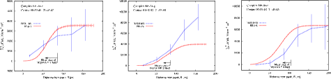
Figure 6.— Azimuthally-integrated brightness plots, of NANTEN and (2’.6-smoothed) Mopra observations of complexes NE-1 (Left), NE-3 (Middle) and NE-4.(Right). Error bars indicate the cumulative sum of the 1$\sigma$ noise level per pixel. Total power measured by Mopra for complexes NE-1 and NE-4 equate with that of NANTEN after some scale, indicating that the same total power is measured over the total area (despite the larger beam size of NANTEN), arguing for an absence of any larger extended CO envelope. Complex NE-3 shows extended emission measured by NANTEN from additional CO components outside and to the east of the area observed by Mopra. Note that the geometry of the observed regions are generally highly irregular, the indicated radii is that of an equivalent-area circle and not the maximum extents of the test areas.

5.3. CO and HI

Wong et al. (2009) have made a thorough comparison of the properties of the Hi and CO emission profiles throughout the LMC. Most notably, they found that CO is detected only towards relatively high Hi column densities, where N(Hi)$\geq$10²¹cm^-1, and that these column densities are a necessary, but insufficient requirement for the formation of CO in the LMC. The Hi found in the LMC exists largely in single-component profiles where it is appropriate to assume that where the centroids of the CO and Hi profiles coincide for a given line of sight, the two components are co-moving and co-evolving. In contrast, the neutral hydrogen component of the SMC is often complex in both position and in velocity: the Hi profiles in the line of sight of the CO emission regions often contain a number of Gaussian components (See Figures 3 and 4), and it is inaccurate to assume that all the Hi found along a particular sight is necessarily associated with the detected CO emission.

To isolate the Hi component that is associated with the CO, we assume that an Hi and CO component must be co-moving, and constrain a multiple-component Gaussian fit with the CO emission velocity centroid as a fixed parameter. We do not assume that the CO and Hi components are similarly turbulence-broadened (i.e. $\Delta$V${}_{CO}\neq\Delta$V_hi).

For this analysis, we first smooth and re-grid the CO dataset to the same geometry as the Hi dataset (i.e. to a 98” beam, and 60” per pixel, which results in some dependence of adjacent pixels). As smoothing dilutes the peak brightness somewhat, we make this test only on the 8 brightest CO clouds; NE-1a,c, NE-3a,c,g and NE-4a,c_lo/hi.

We found in all cases that fitting two Gaussian components provided a significant improvement in the summed reduced $\chi^{2}$ ($\sum\chi_{r}^{2}$) parameter (by a factor of at least two, and a mean improvement by a factor of 4, calculated where T${}_{H{\sc i}}>$3$\sigma_{H{\sc i}}$), but that fitting three components provided no further significant improvement. We have therefore fit two components to the Hi profile and constrained one of them according to the measured CO centroid velocity, as listed in Table 3. In general, constraining one of the two Hi components by the CO velocity centroids did not result in an large degradation of $\sum\chi_{r}^{2}$compared to a completely unconstrained two-component fit: in the unconstrained case, the $\sum\chi_{r}^{2}$ was always of the order unity, while constraining the fit resulted in an average increase of the $\sum\chi_{r}^{2}$ by 20%, although an increase by 40% was found for the most extreme cases. The largest $\sum\chi_{r}^{2}$ value was returned for fitting to cloud NE-3c ($\sum\chi_{r}^{2}$=5.1) and the smallest $\sum\chi_{r}^{2}$ value was returned from fitting to cloud NE-4a ($\sum\chi_{r}^{2}$=1.7). Note that in the case of NE-4, which contains two distinct Hi profiles, fits were made only to the component within the velocity range of interest. For example, while fitting to the high velocity component for NE-4c_high, the low-velocity Hi component was ignored. Constraining one of the fitted HI velocity centroids by the CO component usually resulted in a significant (up to 100%) change in the integrated Hi from a completely unconstrained fit. Clouds NE-1a and NE-1c were the only examples where constraining the fit did not significantly change the measured integrated Hi. An example of this process applied to cloud NE-3c is shown in Figure 7, the integrated intensity of the Hi component associated with each CO velocity centroid is listed in Table 3, and plotted against CO integrated brightness in Figure 8. Figure 8 also shows data from the study of the LMC by Wong et al. (2009).

We do not have a means to presume velocity components to disentangle the complex Hi profiles at positions where CO is not detected. As such, we are unable to make a robust statistical examination of the null case; i.e the values of Integrated Hi where CO is not detected. Figure 8 therefore presents only data-points where both CO and HI are detected, and we find that the ranges of these two qualities are consistent with those in the LMC. As we have observed some of the brightest CO regions in the northern SMC, this suggests that the conclusions made by Wong et al. (2009) regarding the distribution of CO and Hi in the LMC apply also to the SMC: that CO in the northern SMC requires high Hi column densities as a minimum condition for formation. Note that the plot shows that the integrated intensities of the CO clouds in the SMC are generally smaller (by a few factors) than those of the LMC, which is an already-anticipated result (e.g. Israel et al., 1993).

Figure 7.— Two-component fitting made to Hi, where one component is constrained by the velocity centroid (marked with a short vertical line). The $\sum\chi_{r}^{2}$ parameter is shown, indicating a reasonable fit by constrained, two-component fit. The Hi emission over 80-130 km/s is real, but is not fitted nor included in the calculation of $\sum\chi_{r}^{2}$ (see text for details). The heavy solid lines indicate the two fitted components. The lighter solid line is the total fitted result. The heavier dashed line shows the HI brightness temperature (left axis) and the lighter, noisier dashed line shows the CO brightness temperature (right axis).

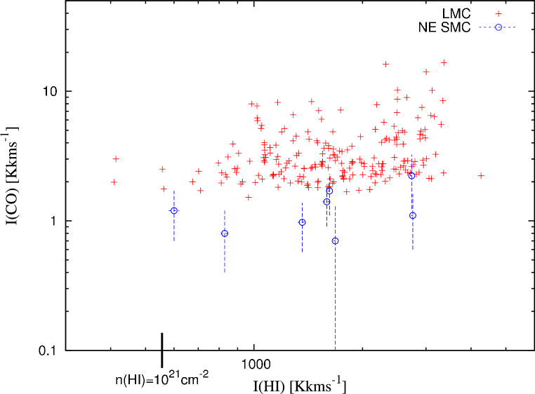
Figure 8.— Plus signs: I_CO/I_HI of Molecular clouds in the LMC Wong et al. (2009).Circles: I_CO/I_HI of Molecular clouds in the SMC. (This publication). CO clouds in the SMC are typically weaker than those in the LMC, and so the SMC data points plot below those of the LMC. Note that the SMC Mopra data are smoothed to the 98” resolution of the Hi dataset. An Hi column density of $n\approx$10²¹ cm^-2 is also indicated with a vertical line, to indicate the $n$Hi star-forming threshold observed in the LMC by Luks & Rohlfs (1992)

Table 3I(CO) and I(HI) of northern CO cloud population

Cloud	IHI	ICO
	[Kkms-1]$\times$103	[Kkms-1]
NE-1a	1.62 $\pm$0.02	1.7 $\pm$0.6
NE-1c	0.830 $\pm$0.02	0.8 $\pm$0.4
NE-3a	1.68 $\pm$0.02	0.7 $\pm$0.6
NE-3c	0.600 $\pm$0.02	1.2 $\pm$0.5
NE-3f	2.76 $\pm$0.03	1.1 $\pm$0.5
NE-4a	1.59 $\pm$0.04	1.4 $\pm$0.5
NE-4chi	1.36 $\pm$0.04	0.9 $\pm$0.4
NE-4clow	2.74 $\pm$0.03	2.2 $\pm$1

5.4. Dust, CO and Hi

Figures 2 B,D and 4C show the relative distribution of the detected CO against that of emission at 160 $\mu$m (Bolatto et al., 2007) for NE-1, NE-3 and NE-4 respectively. We defer a more comprehensive analysis of the relationship of the small-scale CO to the 160 $\mu$m emission to a later paper, however we generally find from these new high-resolution data that the CO clouds in the more quiescent northern SMC are compact and are correlated only with the very brightest peaks of 160 $\mu$m emission; i.e. bright CO occurs only with bright 160 $\mu$m and Hi (e.g. the western CO peak in NE-3), and bright 160 $\mu$m occurs without any detectable CO (e.g. the eastern 160 $\mu$m peak in NE-3).

Variations in the Dust-to-Gas ratio, temperature variations of the dusty component, or photo-disassociation processes may account for inconsistencies in the correlations of the 160 $\mu$m brightness and the CO integrated intensity but the point remains that the correlation of these emission datasets towards the northern SMC is not robust, emphasizing both the need for higher-resolution Hi observations, and also that estimates of the $X$ factor may be highly variable throughout the SMC (see also Leroy et al., 2007).

5.5. Estimates of $X_{CO}$

Our high-resolution observations also allow us to make a new estimate of the SMC $X_{CO}$ factor using virial masses estimated directly from the data. Using the same approach as Pineda et al. (2009); $X\sim M_{vir}/L_{CO}$ (and assuming a ratio the total gas mass to H₂ gas mass of 1.36), we find a range of $X$ factor values of 5.4 $\times$10²⁰ - 4.3 $\times$10²¹ cm^-2[K km s^-1]^-1, with a mean value of 1.3${}^{+1.6}_{-0.8}\times$10²¹ cm^-2[K km s^-1]^-1 for the northern SMC cloud population. The errors of these measurements are high due to the poor signal-to-noise ratio and matching of the beam and cloud radii (as discussed in Section 3). Note that this value is approximately a factor of four higher than that found for the LMC (Pineda et al., 2009) (after adjusting for their slightly different definition of M_vir). Given that the ensemble virial masses (i.e. the velocity dispersions and radii) of the northern SMC population is approximately represented by the smallest members of the LMC cloud population (Pineda et al., 2009), this suggests that the SMC harbors a significantly under-luminous CO-cloud population.

The $X_{SMC}$ factor was also estimated by Rubio et al. (1991) from low-resolution observations of the same northern population. Later $X_{SMC}$ factor estimates were made from higher-resolution observations of the south-west population in SKP-III. These two studies used different methods to estimate the $X_{SMC}$ factor: 1. The earlier paper assumes that the size-line width relationship of CO clouds in the Galaxy and SMC is consistent, and they estimated that SMC CO clouds were under-luminous compared to the Galaxy by a factor of 20. The $X_{SMC}$ was therefore estimated to be $\sim$6$\times$10²¹ cm^-2[K km s^-1]^-1; approximately 20 times higher than $X_{Gal}$. (using the values for $X_{Gal}$ at the time of their writing). 2. The later work by the SEST key projects using $\sim$45” resolution observations of clouds in the southwest of the SMC made estimates of the $X_{SMC}$ for each cloud by assuming a specific fractional mass of the molecular hydrogen. The resulting $X_{SMC}$ values range between 2.5$\times$10²⁰ cm^-2[K km s^-1]^-1 and 2.6$\times$10²² cm^-2[K km s^-1]^-1, with stronger clustering at approximately 10²¹ cm^-2[K km s^-1]^-1. No errors were estimated for these values.

The issue of the relative distributions of CO and H₂ was discussed in some detail by Leroy et al. (2007), who used the 2’.6 FWHM NANTEN data to show that the CO was more compact than the H₂ (determined from 160160 $\mu$m) by a factor of approximately 1.3. They also find that the $X_{SMC}$ factor varies throughout the SMC by a factor of $\sim$2, however, using a factor of 1.3 as a parameter to adjust for the relative sizes of the H₂ and CO emission regions, they estimate a mean $X_{SMC}$ factor of 6$\times$10²¹cm^-2[K km s^-1]^-1. We find from our higher-resolution data that the average radius of the clouds in the SMC is approximately 12 pc, which would result in a correction factor of approximately 3.3 and would adjust their FIR-based estimate of the $X_{SMC}$ to 2.4$\times$10²¹cm^-2[K km s^-1]^-1. This value is consistent with CO-derived virial masses derived earlier. Leroy et al. (2007) indicate that the difference between the mm-derived virial masses and the $\mu$m-derived masses, which would indicate instability and would otherwise lead to cloud fragmentation, may be balanced by an ambient pervasive magnetic field. The small correction found from more exact cloud radii measurements presented here reduces the necessary strength of any such field (see also Bot et al., 2007).

6. summary

We have produced the highest-resolution observations of the molecular cloud population in the northern part of the SMC, to a sensitivity of 210 mK per 0.9 km s^-1 channel and resolving each cloud into 3-7 smaller clouds. We find that this northern population conforms to empirical luminosity-virial mass relationships found for the southern SMC population, yet they are generally much less luminous for their radius. Extrapolating the empirical size-linewidth relationship derived for the southern clouds implies that the northern population has minimum radii of a  4 pc. A comparison with wider-field CO data suggests that two of the three cloud complexes do not exist in a large-scale and weak CO envelope, and that high-resolution Hi data are imperative for more clearly understanding the distribution of molecular material within the SMC. We find that, as for the LMC, CO in the SMC occurs only with high (i.e. $>$10²¹ cm^-1) Hi column density, which suggests that as for the LMC, such column densities are required for its formation. We use these molecular data to estimate X_SMC factors to be approximately 1.3$\times$10²¹, and our high-resolution data allow us to apply a more appropriate correction factor to previous estimates of the X_SMC from $\mu$m+Hi data, and arrive at roughly consistent values.

References

- Bica et al. (2008) Bica, E., Bonatto, C., Dutra, C. M., & Santos, J. F. C. 2008, MNRAS, 389, 678
- Blitz et al. (2007) Blitz, L., Fukui, Y., Kawamura, A., Leroy, A., Mizuno, N., & Rosolowsky, E. 2007, in Protostars and Planets V, ed. B. Reipurth, D. Jewitt, & K. Keil, 81–96
- Bolatto et al. (2008) Bolatto, A. D., Leroy, A. K., Rosolowsky, E., Walter, F., & Blitz, L. 2008, ApJ, 686, 948
- Bolatto et al. (2007) Bolatto, A. D., et al. 2007, ApJ, 655, 212
- Bot et al. (2007) Bot, C., Boulanger, F., Rubio, M., & Rantakyro, F. 2007, A&A, 471, 103
- Cioni et al. (2000) Cioni, M.-R. L., van der Marel, R. P., Loup, C., & Habing, H. J. 2000, A&A, 359, 601
- Davies et al. (1976) Davies, R. D., Elliott, K. H., & Meaburn, J. 1976, MmRAS, 81, 89
- Gooch (1997) Gooch, R. E. 1997, Publications of the Astronomical Society of Australia, 14, 106
- Hughes et al. (In prep.) Hughes, A., et al. In prep.
- Israel et al. (1993) Israel, F. P., et al. 1993, A&A, 276, 25
- Israel et al. (2003) —. 2003, A&A, 406, 817
- Ladd et al. (2005) Ladd, N., Purcell, C., Wong, T., & Robertson, S. 2005, Publications of the Astronomical Society of Australia, 22, 62
- Landman et al. (1982) Landman, D. A., Roussel-Dupre, R., & Tanigawa, G. 1982, ApJ, 261, 732
- Larsen et al. (2000) Larsen, S. S., Clausen, J. V., & Storm, J. 2000, A&A, 364, 455
- Leroy et al. (2007) Leroy, A., Bolatto, A., Stanimirovic, S., Mizuno, N., Israel, F., & Bot, C. 2007, ApJ, 658, 1027
- Luks & Rohlfs (1992) Luks, T., & Rohlfs, K. 1992, A&A, 263, 41
- Maloney & Black (1988) Maloney, P., & Black, J. H. 1988, ApJ, 325, 389
- McKee (1989) McKee, C. F. 1989, ApJ, 345, 782
- Mizuno et al. (2001) Mizuno, A., Yamaguchi, R., Tachihara, K., Toyoda, S., Aoyama, H., Yamamoto, H., Onishi, T., & Fukui, Y. 2001, PASJ, 53, 1071
- Ott et al. (2008) Ott, J., et al. 2008, Publications of the Astronomical Society of Australia, 25, 129
- Pak et al. (1998) Pak, S., Jaffe, D. T., van Dishoeck, E. F., Johansson, L. E. B., & Booth, R. S. 1998, ApJ, 498, 735
- Pineda et al. (2009) Pineda, J. L., Ott, J., Klein, U., Wong, T., Muller, E., & Hughes, A. 2009, ApJ, 703, 736
- Rolleston et al. (2002) Rolleston, W. R. J., Trundle, C., & Dufton, P. L. 2002, A&A, 396, 53
- Rolleston et al. (2003) Rolleston, W. R. J., Venn, K., Tolstoy, E., & Dufton, P. L. 2003, A&A, 400, 21
- Rosolowsky & Leroy (2006) Rosolowsky, E., & Leroy, A. 2006, PASP, 118, 590
- Rubio et al. (2000) Rubio, M., Contursi, A., Lequeux, J., Probst, R., Barbá, R., Boulanger, F., Cesarsky, D., & Maoli, R. 2000, A&A, 359, 1139
- Rubio et al. (1991) Rubio, M., Garay, G., Montani, J., & Thaddeus, P. 1991, ApJ, 368, 173
- Rubio et al. (1993a) Rubio, M., Lequeux, J., & Boulanger, F. 1993a, A&A, 271, 9
- Rubio et al. (1993b) Rubio, M., et al. 1993b, A&A, 271, 1
- Rubio et al. (1996) —. 1996, A&AS, 118, 263
- Stanimirovic (1999) Stanimirovic, S. 1999, PhD thesis, University of Western Sydney, N.S.W, Australia
- Wong et al. (2009) Wong, T., et al. 2009, ApJ, 696, 370