Interplane charge dynamics in a valence-bond dynamical mean-field theory
of cuprate superconductors

Abstract

We present calculations of the interplane charge dynamics in the normal state of cuprate superconductors within the valence-bond dynamical mean-field theory. We show that by varying the hole doping, the $c$-axis optical conductivity and resistivity dramatically change character, going from metallic-like at large doping to insulating-like at low-doping. We establish a clear connection between the behavior of the $c$-axis optical and transport properties and the destruction of coherent quasiparticles as the pseudogap opens in the antinodal region of the Brillouin zone at low doping. We show that our results are in good agreement with spectroscopic and optical experiments.

I Introduction

Even after many years of investigation, cuprate superconductors continue to be at the center of intense experimental and theoretical interest. A key phenomenon which needs to be understood to reveal the nature of superconductivity in the cuprates is the onset of strong momentum-space differentiation in the (hole-) underdoped normal state. This region of the phase diagram is characterized by the suppression of quasiparticle excitations in the antinodal region of the Brillouin zone and the opening of a pseudogap yielding Fermi arcs, as observed, e.g. in angle-resolved photoemission (ARPES) experiments. Damascelli et al. (2003) Other distinctive properties of the cuprates are seen in the extreme anisotropy of the charge dynamics. Ito et al. (1991); Nakamura and Uchida (1993); Takenaka et al. (1994); Basov and Timusk (2005) The in-plane ($\rho_{ab}$) and interplane resistivity ($\rho_{c}$) have different temperature dependence. While $\rho_{ab}$ decreases with decreasing temperatures at all doping levels, $\rho_{c}$ is sensitive to the doping. Its behavior is essentially insulating at low doping, semi-metallic at intermediate doping and metallic in the overdoped regime. The peculiar properties of the interplane charge dynamics have also been observed in optical studies. Basov and Timusk (2005); Tamasaku et al. (1992); Cooper et al. (1993); Homes et al. (1993); Schützmann et al. (1994); Tamasaku et al. (1994); Puchkov et al. (1996a); Basov et al. (1996); Puchkov et al. (1996b) They reveal that the $c$-axis optical conductivity $\sigma_{c}(\Omega)$ shows no sharp Drude peak at low frequencies $\Omega$ in the underdoped normal state. Instead, $\sigma_{c}(\Omega)$ has a rather flat frequency-dependence at temperatures above the pseudogap temperature $T^{*}$. As the temperature is reduced below $T^{*}$, low-energy spectral weight is transferred to higher energies and $\sigma_{c}(\Omega)$ displays a gaplike depression as $\Omega\rightarrow 0$. Only in the highly overdoped region does $\sigma_{c}(\Omega)$ show evidence of emerging coherence. Schützmann et al. (1994)

In this article, we address the interplane charge dynamics of cuprate superconductors within the valence-bond dynamical mean-field theory (VB-DMFT) introduced in Refs. Ferrero et al., 2009a, b. Our results capture many salient features found in experiments for the c-axis resistivity and optical conductivity. Specifically, we show that the opening of a pseudogap in the antinodal region explains the incoherent behavior of the interplane transport.

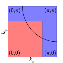
Figure 1: (Color online) The two patches dividing the Brillouin zone. The line shows a non-interacting Fermi surface for the dispersion $\epsilon_{\mathbf{k}}$ of Eq. 1. The central (red) patch covers the nodal region of the Fermi surface, while the border (blue) patch covers the antinodal region.

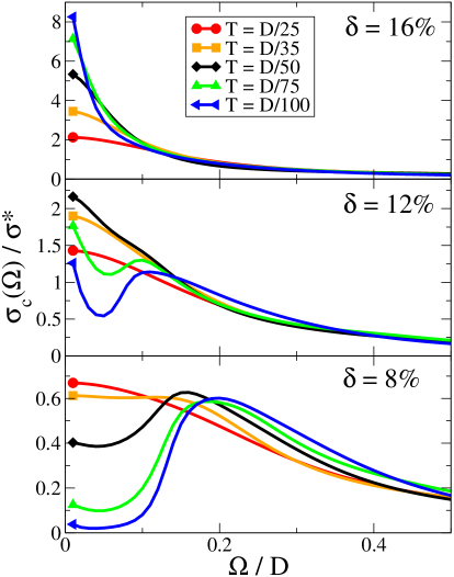
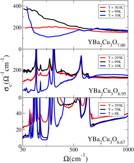
Figure 2: (Color online) Left panel: The $c$-axis optical conductivity $\sigma_{c}(\Omega)$ calculated within VB-DMFT for three doping levels. $\sigma_{c}$ is displayed in units of $\sigma^{*}$ as defined in the text ($\sigma^{*}$ is of order 50 $\Omega^{-1}\mathrm{cm}^{-1}$ for YBa₂Cu₃O_y). Frequency is normalized to the half-bandwidth $D\sim 1\rm{eV}\,=8000\rm{cm}^{-1}$. Right panel: Experimental data for the $c$-axis optical conductivity of YBa₂Cu₃O_y. The data for YBa₂Cu₃O_7.00 is taken from Ref. Schützmann et al., 1994 where the phonon contribution was subtracted by fitting to 5 Lorentzian oscillators. The data for YBa₂Cu₃O_6.95 and YBa₂Cu₃O_6.67 are taken from Refs. LaForge et al., 2008, 2009.

The VB-DMFT is a minimal cluster extension of the dynamical mean-field theory Georges et al. (1996); Maier et al. (2005) that aims at describing momentum-space differentiation together with Mott physics. We apply it to the Hubbard model on a square lattice defined by the Hamiltonian

$$\mathcal{H} = \sum_{\mathbf{k},\sigma}\epsilon_{\mathbf{k}}c^{\dagger}_{\sigma,\mathbf{k}}c^{\phantom{\dagger}}_{\sigma,\mathbf{k}}+U\sum_{i}n_{i\uparrow}n_{i\downarrow},$$ (1)

$$\epsilon_{\mathbf{k}} = -2t[\cos(\mathbf{k}_{x})+\cos(\mathbf{k}_{y})]-4t^{\prime}\cos(\mathbf{k}_{x})\cos(\mathbf{k}_{y}),$$

where $t$ and $t^{\prime}$ are the nearest and next-nearest neighbor hopping and $U$ is the onsite Coulomb repulsion. In the following, we use $U/t=10$ and $t^{\prime}/t=-0.3$, which are values commonly used for modeling hole-doped cuprates in a single-band framework. This value of $U$ is larger than the critical value for the Mott transition in the undoped model, so that we deal with a doped Mott insulator. VB-DMFT is based on an effective two-impurity model embedded in a self-consistent bath. Within this simple approach involving only two degrees of freedom, the lattice self-energy is approximated to be piecewise constant over two patches of the Brillouin zone. These two patches are shown in Fig. 1. Inspired by the phenomenology of cuprate superconductors, their shape is chosen in such a way that the central (red) patch covers the nodal region of the Fermi surface, while the border (blue) patch covers the antinodal region. With this prescription, one degree of freedom of the underlying two-impurity model is associated with the physics of nodal quasiparticles and the other degree of freedom with antinodal quasiparticles. Thank to the relative simplicity of the VB-DMFT approach, it is possible to make very efficient calculations using continuous-time quantum Monte Carlo and obtain accurate spectral functions $A(\mathbf{k},\omega)$. More details concerning this procedure are given in Appendix A and in Refs. Ferrero et al., 2009a, b.

In the VB-DMFT, the formation of Fermi arcs is described by a selective metal-insulator transition in momentum space. Ferrero et al. (2009a, b) Below a doping $\sim 16\%$, the degree of freedom describing the antinodal regions becomes insulating, while that associated to the nodal quasiparticles remains metallic. The orbital-selective mechanism responsible for the pseudogap has also been confirmed in studies involving larger clusters. Gull et al. (2009); Werner et al. (2009); Gull et al. (2010) In Refs. Ferrero et al., 2009a, b, we used the VB-DMFT to compute tunneling and ARPES spectra in good agreement with experiments.

II Interplane optical conductivity

We first compute the frequency-dependent $c$-axis optical conductivity $\sigma_{c}(\Omega)$, given by

$$\begin{split}\sigma_{c}(\Omega)&=\frac{2e^{2}c}{\hbar ab}\int\!\!d\omega\,\frac{f(\omega)-f(\omega+\Omega)}{\Omega}\\ &\quad\frac{1}{N}\sum_{\mathbf{k}}t^{2}_{\perp}(\mathbf{k})A(\mathbf{k},\omega)A(\mathbf{k},\Omega+\omega),\end{split}$$ (2)

where $f$ is the Fermi function, $A(\mathbf{k},\omega)$ the in-plane spectral function, $N$ the number of lattice sites, $e$ the electronic charge, $a,b$ the in-plane lattice constants, $c$ the interplane distance and $t_{\perp}(\mathbf{k})=t_{0}(\cos(\mathbf{k}_{x})-\cos(\mathbf{k}_{y}))^{2}$ is the interplane tunneling matrix element. Andersen et al. (1995); Ioffe and Millis (1998) Note that in this expression $t_{\perp}(\mathbf{k})$ has a strong $\mathbf{k}$-dependence, with contributions stemming mainly from the antinodal region of the Brillouin zone. For convenience, we will express energies in units of the half-bandwidth $D$ of the electronic dispersion, and the optical conductivity in units of $\sigma^{*}=2e^{2}ct_{0}^{2}/\hbar abD^{2}$. In YBa₂Cu₃O_y compounds, $D\sim 1eV\sim 8000\mathrm{cm}^{-1}$ and $\sigma^{*}$ is of order $\sigma^{*}\sim 50\Omega^{-1}\mathrm{cm}^{-1}$.

In the left panel of Fig. 2, we display the computed $\sigma_{c}(\Omega)$ for three levels of hole-doping and several temperatures. Our results show three distinctive behaviors. At high doping $\delta\gtrsim 16\%$, the conductivity displays a metallic-like behavior, with the build-up of a Drude-like peak as the temperature is decreased. Note that as the peak increases additional spectral weight appears at low-energy. At low doping $\delta\lesssim 10\%$, $\sigma_{c}(\Omega)$ is characterized by a gaplike depression at low frequencies where spectral weight is suppressed with decreasing temperature. The width of the gap when it opens at high temperature is $\sim 0.15D$ and remains approximately the same as the temperature is lowered. Note that the spectral weight that is lost in the gap is redistributed over a wide range of energies. The appearance of the depression in the spectra can be directly linked to the formation of a pseudogap in the antinodal region. Ferrero et al. (2009a, b) Indeed, the matrix element $t_{\perp}$ appearing in the expression of the optical conductivity (2) essentially probes the region Chakravarty et al. (1993) close to $(\pm\pi,0),(0,\pm\pi)$ so that a loss of coherent antinodal quasiparticles results in a loss of low-energy spectral weight in the $c$-axis optical conductivity. In Refs. Ferrero et al., 2009a, b, it has been shown that in a zero-temperature analysis of VB-DMFT, coherent quasiparticles disappear in the antinodal region at a doping $\sim 16\%$. This is consistent with $\sigma_{c}$ showing a depression only for doping levels below $\sim 16\%$. At intermediate doping, $\sigma_{c}(\Omega)$ has a mixed character (see left panel of Fig. 2 for $\delta=12\%$). Starting from high temperatures, the low-energy conductivity first displays metallic behavior with an increase in $\sigma_{c}$ as the temperature is lowered. At temperatures $T<D/50$, however, a gap starts to appear and low-energy spectral weight is suppressed.

The right panel of Fig. 2 displays the experimental interplane optical conductivity of YBa₂Cu₃O_y obtained in Refs. Schützmann et al., 1994; LaForge et al., 2008, 2009. At large doping levels, the data shows a build-up of a Drude peak consistent with our theoretical calculation. One must note however that the interplane optical conductivity of YBa₂Cu₃O₇ displays a crossing between the spectra at different temperatures and that the spectral weight transfer is not as clear as in the theoretical curves (left panel) for $\delta=16\%$. In fact, only at doping levels larger than $\delta\sim 25\%$ do the computed $\sigma_{c}$ eventually behave more metallic-like, with a sharp Drude peak at low energies. This behavior is also consistent with other experiments, e.g. on overdoped YBa₂Cu₃O_y, see Fig. 1 of Ref. Schützmann et al., 1995. At low doping, the spectra of YBa₂Cu₃O_6.67 display the opening of a gaplike depression, which is quite well captured by our theoretical results. Remarkably, $\sigma_{c}$ is typically a factor of $10$ smaller that in YBa₂Cu₃O₇, a factor quantitatively similar to what we obtain theoretically by comparing our results for $\delta=16\%$ and $\delta=8\%$. At intermediate doping between these two limits, YBa₂Cu₃O_6.95 displays spectra which depend on temperature in a non-monotonous manner, first increasing upon cooling and then decreasing at lower temperatures. This behavior is indeed observed in our theoretical results at $12\%$ doping. All these observations show that our calculations agree qualitatively, and to a certain extent quantitatively, with optical conductivity measurements on underdoped cuprates (see also e.g. Ref. Basov and Timusk, 2005, Fig. 2 in Ref. Homes et al., 1993 or Fig. 1 in Ref. Homes et al., 2005).

III Interplane resistivity

From the $\Omega=0$ extrapolation of the optical conductivity, we obtain the $c$-axis resistivity $\rho_{c}=1/\sigma_{c}(\Omega=0)$ displayed in Fig. 3 for different doping levels, as a function of temperature. $\rho_{c}$ is displayed in units of $\rho^{*}=1/\sigma^{*}$ which takes the value $\sim 0.02\Omega\mathrm{cm}$ in YBa₂Cu₃O_y. As already discussed for the optical conductivity, the properties of $\rho_{c}$ strongly depend on the doping level. At low doping ($\delta=8\%$), $\rho_{c}(T)$ has an insulating behavior with a large increase as the temperature is lowered. This increase is a direct consequence of the opening of the pseudogap in the antinodal region of the Brillouin zone.

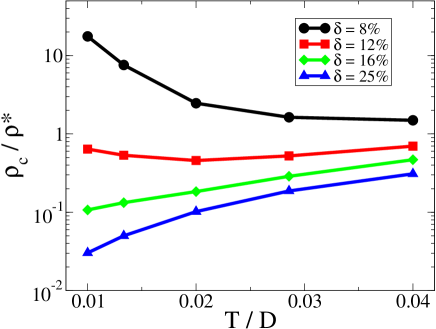
Figure 3: (Color online) The $c$-axis resistivity $\rho_{c}$ calculated within the VB-DMFT for four doping levels as a function of temperature.

As the doping level is increased (see $\delta=12\%$), $\rho_{c}(T)$ starts to display a mixed, non monotonous behavior: it has a minimum as it changes from metallic-like to insulating-like as $T$ decreases. This behavior is indeed observed in interplane resistivity measurements on La_2-xSr_xCuO₄ (Fig. 3 in Ref. Ito et al., 1991, Fig. 2 in Ref. Nakamura and Uchida, 1993), YBa₂Cu₃O_y (Fig. 1 in Ref. Takenaka et al., 1994) or Bi₂Sr₂CaCu₂O_y thin films (inset of Fig. 3 in Ref. Raffy et al., 2007). As we go to higher doping, $\rho_{c}(T)$ eventually acquires a metallic-like behavior with $d\rho_{c}/dT>0$. Note that this metallic behavior emerges from the transfer of spectral weight to lower energies as can be seen from Fig. 2. Moreover, even at the largest doping level $\delta=25\%$, $\rho_{c}(T)$ does not recover the standard Fermi-liquid behavior with $\rho_{c}(T)\sim T^{2}$ (closer inspection instead shows that $\rho_{c}(T)$ roughly behaves as $T^{\alpha}$ with $\alpha\approx 1.6$). One might need to consider even larger doping levels to recover a $T^{2}$ behavior as seen, e.g. in heavily doped La_2-xSr_xCuO₄. Ito et al. (1991)

IV Conclusions

To conclude, in this article we have computed the interplane charge dynamics within the VB-DMFT framework in order to address the properties of the normal-state of high-$T_{c}$ copper-oxide superconductors. Our results show that the interplane charge dynamics of the normal state is characterized by three regimes. (i) An overdoped regime where both the $c$-axis optical conductivity and resistivity show a metallic-like behavior. (ii) An underdoped regime where the destruction of coherent quasiparticles in the antinodal region induces a gaplike depression in $\sigma_{c}$ and a resulting insulating-like interlayer resistivity which increases as temperature is lowered. (iii) An intermediate-doping mixed regime with first the buildup of a coherence peak in $\sigma_{c}$ as the temperature is decreased, followed by a loss of low-energy spectral weight as the pseudogap opens at lower temperatures. As a consequence, $\rho_{c}$ has a non-monotonic behavior with a minimum at intermediate temperature. Our calculations are in good agreement with spectroscopic and transport experiments.

Appendix A Details about the VB-DMFT approach

Let us give here some technical details and briefly describe how our results were obtained. Within the VB-DMFT, the effective model that one has to solve is a two-impurity Anderson model Ferrero et al. (2009a, b). The even (+) combination of the two impurity orbitals is associated with the nodal part of the Brillouin zone, while the odd (-) combination is associated to the antinode. The Anderson impurity model is solved using a continuous-time quantum Monte Carlo algorithm (CTQMC) Werner et al. (2006); Werner and Millis (2006) that yields the even (resp. odd) orbital self-energy $\Sigma_{+}(i\omega_{n})$ (resp. $\Sigma_{-}(i\omega_{n})$) at the Matsubara frequencies $i\omega_{n}$. At this stage one can readily get the quasiparticle residues by carefully extrapolating $\Sigma_{\pm}(i\omega_{n})$ at zero frequency

$$Z_{\pm}=\Big{(}1-\frac{d\mathrm{Im}\Sigma_{\pm}(i\omega_{n})}{d\omega_{n}}\Big{|}_{\omega_{n}\rightarrow 0}\Big{)}^{-1}.$$ (3)

The inverse quasiparticle lifetime is then given by

$$\Gamma_{\pm}=-Z_{\pm}\mathrm{Im}\Sigma_{\pm}(i\omega_{n})\Big{|}_{\omega_{n}\rightarrow 0}.$$ (4)

Finally, the nodal ($\Gamma_{\mathrm{N}}$) and antinodal ($\Gamma_{\mathrm{AN}}$) inverse lifetimes are associated with $\Gamma_{+}$ and $\Gamma_{-}$ respectively. In order to compute the optical conductivity and the resistivities it is necessary to have access to the in-plane spectral function $A(\mathbf{k},\omega)$. A first step is to analytically continue the self-energies $\Sigma_{\pm}$ on the real-frequency axis, which is achieved using Padé approximants. Vidberg and Serene (1977) This is made possible thank to the extremely accurate, low-noise imaginary-time data. A second step is to interpolate the self-energy to obtain a $\mathbf{k}$-dependent $\Sigma(\mathbf{k},\omega)$ from which the spectral function will be computed. Refs. Ferrero et al., 2009a, b have shown that an efficient interpolation procedure is the $M$-interpolation. Stanescu and Kotliar (2006); Stanescu et al. (2006) The self-energy is obtained with $\Sigma(\mathbf{k},\omega)=\omega+\mu-M(\mathbf{k},\omega)^{-1}$, where the cumulant $M(\mathbf{k},\omega)$ is given by

$$M(\mathbf{k},\omega)=\frac{\alpha_{+}(\mathbf{k})}{\omega+\mu-\Sigma_{+}(\omega)}+\frac{\alpha_{-}(\mathbf{k})}{\omega+\mu-\Sigma_{-}(\omega)},$$ (5)

with $\alpha_{\pm}(\mathbf{k})=\frac{1}{2}\{1\pm\frac{1}{2}[\cos(\mathbf{k}_{x})+\cos(\mathbf{k}_{y})]\}$. Finally, the spectral function is computed with

$$A(\mathbf{k},\omega)=\frac{1}{\omega+\mu-\epsilon_{\mathbf{k}}-\Sigma(\mathbf{k},\omega)},$$ (6)

where $\epsilon_{\mathbf{k}}$ is the square lattice dispersion.

References

- Damascelli et al. (2003) A. Damascelli, Z. Hussain, and Z.-X. Shen, Rev. Mod. Phys. 75, 473 (2003).
- Ito et al. (1991) T. Ito, H. Takagi, S. Ishibashi, T. Ido, and S. Uchida, Nature 350, 596 (1991).
- Nakamura and Uchida (1993) Y. Nakamura and S. Uchida, Phys. Rev. B 47, 8369 (1993).
- Takenaka et al. (1994) K. Takenaka, K. Mizuhashi, H. Takagi, and S. Uchida, Phys. Rev. B 50, 6534 (1994).
- Basov and Timusk (2005) D. N. Basov and T. Timusk, Rev. Mod. Phys. 77, 721 (2005).
- Cooper et al. (1993) S. L. Cooper, D. Reznik, A. Kotz, M. A. Karlow, R. Liu, M. V. Klein, W. C. Lee, J. Giapintzakis, D. M. Ginsberg, B. W. Veal, et al., Phys. Rev. B 47, 8233 (1993).
- Homes et al. (1993) C. C. Homes, T. Timusk, R. Liang, D. A. Bonn, and W. N. Hardy, Phys. Rev. Lett. 71, 1645 (1993).
- Schützmann et al. (1994) J. Schützmann, S. Tajima, S. Miyamoto, and S. Tanaka, Phys. Rev. Lett. 73, 174 (1994).
- Tamasaku et al. (1992) K. Tamasaku, Y. Nakamura, and S. Uchida, Phys. Rev. Lett. 69, 1455 (1992).
- Tamasaku et al. (1994) K. Tamasaku, T. Ito, H. Takagi, and S. Uchida, Phys. Rev. Lett. 72, 3088 (1994).
- Puchkov et al. (1996a) A. V. Puchkov, D. N. Basov, and T. Timusk, J. Phys. Cond. Matt. 8, 10049 (1996a).
- Basov et al. (1996) D. N. Basov, R. Liang, B. Dabrowski, D. A. Bonn, W. N. Hardy, and T. Timusk, Phys. Rev. Lett. 77, 4090 (1996).
- Puchkov et al. (1996b) A. V. Puchkov, P. Fournier, D. N. Basov, T. Timusk, A. Kapitulnik, and N. N. Kolesnikov, Phys. Rev. Lett. 77, 3212 (1996b).
- Ferrero et al. (2009a) M. Ferrero, P. S. Cornaglia, L. D. Leo, O. Parcollet, G. Kotliar, and A. Georges, Europhys. Lett. 85, 57009 (2009a).
- Ferrero et al. (2009b) M. Ferrero, P. S. Cornaglia, L. D. Leo, O. Parcollet, G. Kotliar, and A. Georges, Phys. Rev. B 80, 064501 (2009b).
- LaForge et al. (2008) A. D. LaForge, W. J. Padilla, K. S. Burch, Z. Q. Li, A. A. Schafgans, K. Segawa, Y. Ando, and D. N. Basov, Phys. Rev. Lett. 101, 097008 (2008).
- LaForge et al. (2009) A. D. LaForge, W. J. Padilla, K. S. Burch, Z. Q. Li, A. A. Schafgans, K. Segawa, Y. Ando, and D. N. Basov, Phys. Rev. B 79, 104516 (2009).
- Georges et al. (1996) A. Georges, G. Kotliar, W. Krauth, and M. J. Rozenberg, Rev. Mod. Phys. 68, 13 (1996).
- Maier et al. (2005) T. Maier, M. Jarrell, T. Pruschke, and M. H. Hettler, Rev. Mod. Phys. 77, 1027 (2005).
- Gull et al. (2009) E. Gull, O. Parcollet, P. Werner, and A. J. Millis, Phys. Rev. B 80, 245102 (2009).
- Werner et al. (2009) P. Werner, E. Gull, O. Parcollet, and A. J. Millis, Phys. Rev. B 80, 045120 (2009).
- Gull et al. (2010) E. Gull, M. Ferrero, O. Parcollet, A. Georges, and A. J. Millis (2010), arXiv:1007.2592.
- Andersen et al. (1995) O. K. Andersen, A. I. Liechtenstein, O. Jepsen, and F. Paulsen, J. Phys. Chem. Solids 56, 1573 (1995).
- Ioffe and Millis (1998) L. B. Ioffe and A. J. Millis, Phys. Rev. B 58, 11631 (1998).
- Chakravarty et al. (1993) S. Chakravarty, A. S. and. P. W. Anderson, and S. Strong, Science 261, 337 (1993).
- Schützmann et al. (1995) J. Schützmann, S. Tajima, S. Miyamoto, and S. Tanaka, J. Phys. Chem. Solids 56, 1839 (1995).
- Homes et al. (2005) C. C. Homes, S. V. Dordevic, D. A. Bonn, R. Liang, W. N. Hardy, and T. Timusk, Phys. Rev. B 71, 184515 (2005).
- Raffy et al. (2007) H. Raffy, V. Toma, C. Murrills, and Z. Z. Li, Physica C 460-462, 851 (2007).
- Werner et al. (2006) P. Werner, A. Comanac, L. de’ Medici, M. Troyer, and A. J. Millis, Phys. Rev. Lett. 97, 076405 (2006).
- Werner and Millis (2006) P. Werner and A. J. Millis, Phys. Rev. B 74, 155107 (2006).
- Vidberg and Serene (1977) H. J. Vidberg and J. W. Serene, J. Low Temp. Phys. 29, 179 (1977).
- Stanescu and Kotliar (2006) T. D. Stanescu and G. Kotliar, Phys. Rev. B 74, 125110 (2006).
- Stanescu et al. (2006) T. D. Stanescu, M. Civelli, K. Haule, and G. Kotliar, Ann. Phys. 321, 1682 (2006).