Hidden regular variation: Detection and Estimation

Abstract.

Hidden regular variation defines a subfamily of distributions satisfying regular variation on $\mathbb{E}=[0,\infty]^{d}\backslash\{(0,0,\cdots,0)\}$ and models another regular variation on the sub-cone $\mathbb{E}^{(2)}=\mathbb{E}\backslash\cup_{i=1}^{d}\mathbb{L}_{i}$, where $\mathbb{L}_{i}$ is the $i$-th axis. We extend the concept of hidden regular variation to sub-cones of $\mathbb{E}^{(2)}$ as well. We suggest a procedure for detecting the presence of hidden regular variation, and if it exists, propose a method of estimating the limit measure exploiting its semi-parametric structure. We exhibit examples where hidden regular variation yields better estimates of probabilities of risk sets.

Keywords: Regular variation; vague convergence; weak convergence; spectral measure; risk sets.

1. Introduction

Multivariate risks with Pareto-like tails are usually modeled using the theory of regular variation on cones. Let $\mathbb{C}$ be a cone in $[-\infty,\infty]^{d}$ satisfying $\boldsymbol{x}\in\mathbb{C}$ implies $t\boldsymbol{x}\in\mathbb{C}$ for $t>0$ and denote the set of all non-negative Radon measures on $\mathbb{C}$ by $M_{+}(\mathbb{C}).$ The distribution of a random vector ${\bf{Z}}$ is regularly varying on $\mathbb{C}$ if there exist a scaling function $g(t)\uparrow\infty,$ and a non-zero Radon measure $\chi\in M_{+}(\mathbb{C})$ such that

(1.1) $$tP\left[\frac{{\bf{Z}}}{g(t)}\in\cdot\right]\stackrel{{\scriptstyle v}}{{\rightarrow}}\chi(\cdot)$$

in $M_{+}(\mathbb{C}),$ where $\stackrel{{\scriptstyle v}}{{\rightarrow}}$ denotes vague convergence [29]. Risks with heavy tails could also be modeled by stable distributions on a general convex cone; see [8].

Suppose the distribution of a random vector ${\bf{Z}}$ is regularly varying on the first quadrant $\operatorname{\mathbb{E}}:=[0,\infty]^{d}\backslash\{(0,0,\cdots 0)\}$ as in (1.1) with limit measure $\nu$. It is possible for $\nu$ to give zero mass to a proper sub-cone $\mathbb{C}{\subset}\operatorname{\mathbb{E}};$ for example, we could have

$$\mathbb{C}=\operatorname{\mathbb{E}}^{(2)}=\mathbb{E}\backslash\cup_{1\leq j_{1}<j_{2}<\cdots<j_{d-1}\leq d}\{x^{j_{1}}=0,\cdots,x^{j_{d-1}}=0\},$$

the first quadrant with the axes removed. If the distribution of $\bf{Z}$ is also regularly varying on the subcone $\mathbb{C}$ with scaling function $g_{\mathbb{C}}(t)\uparrow\infty$ and $g(t)/g_{\mathbb{C}}(t)\to\infty$, then we say the distribution of $\bf{Z}$ possesses hidden regular variation (HRV) on $\mathbb{C}$. HRV helps detect finer structure that may be ignored by regular variation on $\operatorname{\mathbb{E}}.$ We will later refine our definition of hidden regular variation for a finite sequence of cones $\operatorname{\mathbb{E}}\supset\mathbb{C}_{1}\supset\mathbb{C}_{2}\supset\cdots\mathbb{C}_{m}$.

Failure of regular variation on $\operatorname{\mathbb{E}}$ to distinguish between independence and asymptotic independence prodded Ledford and Tawn [19, 20] to define the coefficient of tail dependence and this idea was extended to hidden regular variation on $\operatorname{\mathbb{E}}^{(2)}$ in [26]. See also [5, 9, 12, 15, 18, 21, 22, 23, 24, 27, 32].

Hidden regular variation provides models that possess regular variation on $\operatorname{\mathbb{E}}$ and asymptotic independence [28, pages 323-325]. The concept has typically been considered in two dimensions using the sub-cone $\operatorname{\mathbb{E}}^{(2)}$. It is not clear how best to extend the ideas of HRV to dimensions higher than two and one obvious remark is that how one proceeds with definitions depends on the sort of risk regions being considered.

To demonstrate what is possible in higher dimensions, in this paper we define hidden regular variation on the sub-cones

$$\operatorname{\mathbb{E}}^{(l)}=[0,\infty]^{d}\backslash\cup_{1\leq j_{1}<j_{2}<\cdots<j_{d-l+1}\leq d}\{x^{j_{1}}=0,\cdots,x^{j_{d-l+1}}=0\},\quad 3\leq l\leq d,$$

of $\operatorname{\mathbb{E}}$ and show with an example that asymptotic independence is not a necessary condition for HRV on $\operatorname{\mathbb{E}}^{(l)},\hskip 2.84544pt3\leq l\leq d.$ Hidden regular variation on $\operatorname{\mathbb{E}}^{(l)},$ means that the distribution of the random vector ${\bf{Z}}$ is regularly varying on $\operatorname{\mathbb{E}}$ as in (1.1) with limit measure $\nu$ and $\nu(\operatorname{\mathbb{E}}^{(l-1)})>0,$ but $\nu(\operatorname{\mathbb{E}}^{(l)})=0.$ Also, there is a scaling function $g_{\operatorname{\mathbb{E}}^{(l)}}(t)$ satisfying $g(t)/g_{\operatorname{\mathbb{E}}^{(l)}}(t)\to\infty$ which makes the distribution of ${\bf{Z}}$ regularly varying on the cone $\operatorname{\mathbb{E}}^{(l)}$ as in (1.1) with limit measure $\nu^{(l)}$. Later, when we define HRV on the finite sequence of cones $\operatorname{\mathbb{E}}\supset\operatorname{\mathbb{E}}^{(2)}\supset\cdots\supset\operatorname{\mathbb{E}}^{(d)},$ our definition of HRV on $\operatorname{\mathbb{E}}^{(l)}$ will be modified accordingly. We suggest exploratory methods for detecting the presence of hidden regular variation on $\operatorname{\mathbb{E}}^{(l)},\hskip 2.84544pt2\leq l\leq d.$ The existing method of detecting hidden regular variation on $\operatorname{\mathbb{E}}^{(2)}$ is valid only for dimension $d=2,$ but our detection methods are applicable for any finite dimension.

If exploratory detection methods confirm data is consistent with the hypothesis of regular variation on a cone $\operatorname{\mathbb{E}}^{(l)}$ as in (1.1), we must estimate the limit measure $\nu^{(l)}$. Previous methods [15] for estimating the limit measure $\nu^{(2)}$ of hidden regular variation on $\mathbb{E}^{(2)}$ have been non-parametric and ignored the semi-parametric structure of $\nu^{(2)}.$ We offer some improvement by exploiting the semi-parametric structure of $\nu^{(2)}$ and estimate the parametric and non-parametric parts of $\nu^{(2)}$ separately.

On $\mathbb{E}$, estimation of the limit measure of regular variation is resolved by the familiar method of the polar coordinate transformation ${\bf{x}}\to(||{\bf{x}}||,{{\bf{x}}}/{||{\bf{x}}||});$ after this transformation, the limit measure $\nu$ is a product of a probability measure $S$ and a Pareto measure $\nu_{\alpha}$, $\nu_{\alpha}((r,\infty])=r^{-\alpha},r>0$ [28, pages 168-179]. Trying to decompose $\nu^{(2)}$ in this way presents the difficulty that the decomposition gives a Pareto measure $\nu_{\alpha^{(2)}}$ and a possibly infinite Radon measure [28, pages 324-339]. So we transform to a different coordinate system after which $\nu^{(2)}$ is a product of a Pareto measure $\nu_{\alpha^{(2)}}$ and a probability measure $S^{(2)}$ on $\delta\aleph^{(2)}=\{{\bf{x}}\in\operatorname{\mathbb{E}}^{(2)}:x^{(2)}=1\}$, where $x^{(2)}$ is the second largest component of $\boldsymbol{x}$. We call the probability measure $S^{(2)}$ the hidden angular measure on $\operatorname{\mathbb{E}}^{(2)}.$ We suggest procedures for consistently estimating the parameter $\alpha^{(2)}$ of the Pareto measure $\nu_{\alpha^{(2)}}$ and the hidden angular measure $S^{(2)}$ and explain how these estimates lead to an estimate of $\nu^{(2)}$. If HRV on $\operatorname{\mathbb{E}}^{(l)}$ is present for some $3\leq l\leq d,$ there is a similar transformation of coordinates making $\nu^{(l)}$ a product of a Pareto measure $\nu_{\alpha^{(l)}}$ and a probability measure $S^{(l)}$ on $\delta\aleph^{(l)}=\{{\bf{x}}\in\operatorname{\mathbb{E}}^{(l)}:x^{(l)}=1\},$ where $x^{(l)}$ is the $l$-th largest component of $\boldsymbol{x}$. We call this probability measure $S^{(l)}$, the hidden angular measure on $\operatorname{\mathbb{E}}^{(l)}$ and employ similar estimation methods for $l\geq 3$ as we did for $l=2$.

For empirical exploration of the spectral or hidden spectral measures, it is often desirable to make density plots. However, the hidden spectral measure $S^{(l)}$ is supported on $\delta\aleph^{((l)}$, which is a difficult plotting domain. For example, when $d=3,$ the set $\delta\aleph^{(2)}$ is a disjoint union of six rectangles lying on three different planes as shown in Figure 1. Though $\delta\aleph^{(l)}$ is a $(d-1)$-dimensional set, $d$-dimensional vectors are needed to represent $\delta\aleph^{(l)}$. So, the density plots on $\delta\aleph^{(l)}$ also requires an additional dimension. In the two dimensional case, the problem is resolved by taking a transformation of points from $\delta\aleph^{(1)}=\{{\bf{x}}\in\operatorname{\mathbb{E}}:x^{(1)}=1\}$ to $[0,1]$ and looking at the density of the induced probability measure of the transformed points [28, pages 316-321]. We seek similar appropriate transformations in higher dimensional cases. We devise a transformation of points from $\delta\aleph^{(l)}$ to the $(d-1)$-dimensional simplex $\Delta_{d-1}=\{{\bf{x}}\in[0,1]^{d-1}:\sum_{i=1}^{d-1}x^{i}\leq 1\}$ (see Section 4.1). The probability measure $\tilde{S}^{(l)}$ on the transformed points induced by $S^{(l)}$ is called the transformed (hidden) spectral measure. Since the set $\Delta_{d-1}$ is represented by $(d-1)$-dimensional vectors, the problem of incorporating an additional dimension in the density plots vanishes.

Figure 1. The shaded region shows the set $\delta\aleph^{(2)},$ when $d=3$.

For characterizations of hidden regular variation [21] it is useful to know if $\nu^{(l)}(\{{\bf{x}}\in\operatorname{\mathbb{E}}^{(l)}:||{\bf{x}}||>1\})$ is finite or not, where $||{\bf{x}}||$ is any norm of ${\bf{x}}$. Such knowledge is also useful for estimating probabilities of some risk sets. For example, if $\nu^{(l)}(\{{\bf{x}}\in\operatorname{\mathbb{E}}^{(l)}:||{\bf{x}}||>1\})$ is finite, then so is $\nu^{(l)}(\{{\bf{x}}\in\operatorname{\mathbb{E}}^{(l)}:a_{1}x^{1}+a_{2}x^{2}+\cdots+a_{d}x^{d}>y\},a_{i}>0,i=1,2,\cdots,d,y>0$. We show that this issue can be resolved by checking a moment condition.

1.1. Outline

Section 1.2 explains notation. In Section 2, we review the definitions of regular variation on $\operatorname{\mathbb{E}}$ and hidden regular variation on $\operatorname{\mathbb{E}}^{(2)}$, and extend the concept to the sub-cones $\operatorname{\mathbb{E}}^{(l)}=[0,\infty]^{d}\backslash\cup_{1\leq j_{1}<j_{2}<\cdots<j_{d-l+1}\leq d}\{x^{j_{1}}=0,\cdots,x^{j_{d-l+1}}=0\}$, $3\leq l\leq d.$ Section 3 discusses exploratory detection techniques for hidden regular variation on $\operatorname{\mathbb{E}}^{(l)}$ and estimation of the limit measure $\nu^{(l)}.$ We consider in Section 4 a transformation that allows us to visualize the hidden angular measure $S^{(l)}$ through another probability measure $\tilde{S}^{(l)}$ on the $(d-1)$-dimensional simplex. In Section 5, we discuss conditions for $\nu^{(l)}(\{{\bf{x}}\in\operatorname{\mathbb{E}}^{(l)}:||{\bf{x}}||>1\})$ being finite or not. Section 6 gives examples of risk sets where hidden regular variation helps in obtaining finer estimates of their probabilities. Our methodologies are applied to two examples in Section 7. We conclude with some remarks and outline open issues in Section 8.

1.2. Notation

1.2.1. Vectors and cones

For denoting a vector and its components, we use:

$${\bf{x}}=(x^{1},x^{2},\cdots,x^{d}),\hskip 28.45274ptx^{i}=\hbox{$i$-th component of }{\bf{x}},\hskip 2.84544pti=1,2,\cdots,d.$$

The vectors of all zeros, all ones and all infinities are denoted by ${\bf{0}}=(0,0,\cdots,0),$ ${\bf{1}}=(1,1,\cdots,1)$ and ${\boldsymbol{\infty}}=(\infty,\infty,\cdots,\infty)$ respectively. Operations on and between vectors are understood componentwise. In particular, for non-negative vectors $\boldsymbol{x}$ and ${\boldsymbol{\beta}}=(\beta^{1},\beta^{2},\cdots,\beta^{d})$, write ${\bf{x}}^{{\boldsymbol{\beta}}}=({(x^{1})}^{\beta^{1}},{(x^{2})}^{\beta^{2}},\cdots,{(x^{d})}^{\beta^{d}})$. We denote the norm of ${\bf{x}}$ as $||{\bf{x}}||$. Unless specified, this could be taken as any norm. For the $i$-th largest component of ${\bf{x}}$, we use:

$$x^{(i)}=\hbox{$i$-th largest component of }{\bf{x}},\hskip 2.84544pti=1,2,\cdots,d,\hskip 8.5359pt\hbox{i.e.}\hskip 8.5359ptx^{(1)}\geq x^{(2)}\geq\cdots\geq x^{(d)}.$$

So, the superscripts denote components of a vector and the ordered component is denoted by a parenthesis in the superscript.

Sometimes, we have to sort the $i$-th largest components of the vectors ${\bf{Z}}_{1},{\bf{Z}}_{2},\cdots,{\bf{Z}}_{n}$ in non-increasing order. We first obtain the vector $\{Z_{1}^{(i)},Z_{2}^{(i)},\cdots,Z_{n}^{(i)}\}$ by taking the $i$-th largest component for each ${\bf{Z}}_{j}$ and then sort these to get

$$Z_{(1)}^{(i)}\geq Z_{(2)}^{(i)}\geq\cdots\geq Z_{(n)}^{(i)}.$$

We use the parentheses in the subscript to avoid double parentheses on the superscript.

The cones we consider are

$$\operatorname{\mathbb{E}}= \operatorname{\mathbb{E}}^{(1)}=[0,\infty]^{d}\backslash\{{\bf{0}}\}=[0,\infty]^{d}\backslash\{x^{1}=0,\cdots,x^{d}=0\}$$

$$= [0,\infty]^{d}\backslash\{x^{(1)}=0\}=\{\boldsymbol{x}\in[0,\infty]^{d}:x^{(1)}>0\}$$

and for $2\leq l\leq d$,

$$\operatorname{\mathbb{E}}^{(l)}= [0,\infty]^{d}\backslash\cup_{1\leq j_{1}<j_{2}<\cdots<j_{d-l+1}\leq d}\{x^{j_{1}}=0,\cdots,x^{j_{d-l+1}}=0\}$$

$$= [0,\infty]^{d}\backslash\{x^{(l)}=0\}=\{\boldsymbol{x}\in[0,\infty]^{d}:x^{(l)}>0\}.$$

For $2\leq l\leq d,$ $\operatorname{\mathbb{E}}^{(l)}$ is the set of points in $\operatorname{\mathbb{E}}$ such that at least $l$ components are positive. Sometimes $\operatorname{\mathbb{E}}^{(2)}$ is expressed as $\operatorname{\mathbb{E}}^{(2)}=\operatorname{\mathbb{E}}\backslash\cup_{i=1}^{d}\mathbb{L}_{i}$, where $\mathbb{L}_{i}:=\{t{\bf{e}}_{i},t>0\}$ is the $i$-th axis and ${\bf{e}}_{i}=(0,\ldots,0,1,0,\ldots,0)$, where $1$ is in the $i$-th position, $i=1,2,\ldots,d$. For ${\bf{x}}\in\operatorname{\mathbb{E}},$ we use $[{\bf{0,x}}]^{c}$ to mean $[{\bf{0,x}}]^{c}=\operatorname{\mathbb{E}}\backslash[{\bf{0,x}}]=\{{\bf{y}}\in\operatorname{\mathbb{E}}:\vee_{i=1}^{d}{y^{i}}/{x^{i}}>1\}.$

1.2.2. Regular variation and vague convergence.

We express vague convergence [28, page 173] of Radon measures as $\stackrel{{\scriptstyle v}}{{\rightarrow}}$ and weak convergence of probability measures [1, page 14] as $\Rightarrow$. Denote the set of non-negative Radon measures on a space $\mathbb{F}$ as $M_{+}(\mathbb{F})$ and the set of all non-negative continuous functions with compact support from $\mathbb{F}$ to $\mathbb{R}^{+}$ as $C_{K}^{+}(\mathbb{F})$. The notation $RV_{\rho}$ means the family of one dimensional regularly varying functions with exponent of variation $\rho$ ([28, page 24], [2, 10]). For any measure $m$ and a real-valued function $f$, denote the integral $\int f({\bf{x}})m(dx)$ by $m(f)$.

For defining regular variation of distributions of random vectors on $\operatorname{\mathbb{E}}=\operatorname{\mathbb{E}}^{(1)}$ as in (1.1), we use the scaling function $b(t)=b^{(1)}(t)$ and get the limit measure $\nu=\nu^{(1)}$. Similarly, for defining regular variation of distributions of random vectors on $\operatorname{\mathbb{E}}^{(l)}$, $2\leq l\leq d$, we use the scaling function $b^{(l)}(t)$ and get the limit measure $\nu^{(l)}$. For each $1\leq l\leq d$, define the set $\aleph^{(l)}$ by $\aleph^{(l)}=\{{\bf{x}}\in\operatorname{\mathbb{E}}^{(l)}:x^{(l)}\geq 1\}$. Since $\aleph^{(l)}$ is compact in $\operatorname{\mathbb{E}}^{(l)}$, there always exists a suitable choice of the scaling function $b^{(l)}(t)$ which makes $\nu^{(l)}(\aleph^{(l)})=1.$ We assume this from now on.

For each $2\leq l\leq d$, if we have hidden regular variation on $\operatorname{\mathbb{E}}^{(l)}$, the limit measure $\nu^{(l)}$ can be expressed in a convenient coordinate system as a product of a Pareto measure $\nu_{\alpha^{(l)}}(dr)=\alpha^{(l)}r^{-\alpha^{(l)}-1}dr,\,r>0$ and a probability measure $S^{(l)}$ on the compact set $\delta\aleph^{(l)}=\{{\bf{x}}\in\operatorname{\mathbb{E}}^{(l)}:x^{(l)}=1\}$. The measure $S^{(l)}$ is called the hidden angular or hidden spectral measure on $\operatorname{\mathbb{E}}^{(l)}.$ Whenever $\nu^{(l)}(\{{\bf{x}}\in\operatorname{\mathbb{E}}^{(l)}:x^{(l)}\geq 1,x^{(1)}=\infty\})=0,$ we view $S^{(l)}$ through its transformed version denoted $\tilde{S}^{(l)}$, which is a probability measure on the $(d-1)$-dimensional simplex $\Delta_{d-1}=\{{\bf{x}}\in[0,1]^{d-1}:\sum_{i=1}^{d-1}x^{i}\leq 1\}$.

1.2.3. Anti-ranks.

Suppose, ${\bf{Z}}_{1},{\bf{Z}}_{2},\cdots,{\bf{Z}}_{n}$ are random vectors in ${[0,\infty)}^{d}$. For $j=1,2,\ldots,d$, $i=1,2,\cdots,n$, define the anti-rank

$$r_{i}^{j}=\sum_{l=1}^{n}1_{\{Z_{l}^{j}\geq Z_{i}^{j}\}}$$

for $Z_{i}^{j}$ to be the number of $j$-th components greater than or equal to $Z_{i}^{j}$. For $2\leq l\leq d$, define

$$m_{i}^{(l)}=\hbox{the $l$-th largest component of}\hskip 5.69046pt(\frac{1}{r_{i}^{j}},j=1,2,\ldots,d)$$

and then order them as

$$m_{(1)}^{(l)}\geq m_{(2)}^{(l)}\geq\cdots\geq m_{(n)}^{(l)}.$$

2. Hidden regular variation

We give more details about regular variation on $\operatorname{\mathbb{E}}$ and HRV on $\operatorname{\mathbb{E}}^{(2)}$ and then extend the definitions to hidden regular variation on sub-cones of $\operatorname{\mathbb{E}}^{(2)}$. We illustrate with some examples.

2.1. Hidden regular variation on $\operatorname{\mathbb{E}}^{(2)}$

Consider regular variation on $\operatorname{\mathbb{E}}$ and hidden regular variation on $\operatorname{\mathbb{E}}^{(2)}$.

2.1.1. The standard case

The distribution of ${\bf{Z}}=(Z^{1},Z^{2},\cdots,Z^{d})$ is regularly varying on $\operatorname{\mathbb{E}}:=[0,\infty]^{d}\backslash\{{\bf{0}}\}$ with limit measure $\nu$ if there exist a function $b(t)\uparrow\infty$ as $t\to\infty$ and a non-negative non-degenerate Radon measure $\nu\neq 0$ such that

(2.1) $$tP\left[\frac{{\bf{Z}}}{b(t)}\in\cdot\right]\stackrel{{\scriptstyle v}}{{\rightarrow}}\nu(\cdot)\quad\text{in $M_{+}(\operatorname{\mathbb{E}})$}.$$

The limit measure $\nu$ must have all non-zero marginals. Then, there exists $\alpha>0$ such that $b(\cdot)\in RV_{1/\alpha}$ and $\nu$ satisfies the scaling property

(2.2) $$\nu(c\cdot)=c^{-\alpha}\nu(\cdot),\hskip 28.45274ptc>0.$$

Call the limit relation (2.1) the standard case which requires the same scaling function $b(t)$ for all the components of ${\bf{Z}}$ in (2.1) and ensures that $\nu$ has all non-zero marginals.

HRV allows for another regular variation on a sub-cone such as $\operatorname{\mathbb{E}}^{(2)}$. The distribution of ${\bf{Z}}$ has hidden regular variation on $\operatorname{\mathbb{E}}^{(2)}$ if in addition to (2.1) there exist a non-decreasing function $b^{(2)}(t)\uparrow\infty$ such that $b(t)/b^{(2)}(t)\to\infty$ and a non-negative Radon measure $\nu^{(2)}\neq 0$ on $\operatorname{\mathbb{E}}^{(2)}$ such that

(2.3) $$tP\left[\frac{{\bf{Z}}}{b^{(2)}(t)}\in\cdot\right]\stackrel{{\scriptstyle v}}{{\rightarrow}}\nu^{(2)}(\cdot)\quad\text{in $M_{+}(\operatorname{\mathbb{E}}^{(2)})$};$$

see [28, page 324]. It follows from (2.3) that there exists $\alpha^{(2)}\geq\alpha$ such that $b^{(2)}(\cdot)\in RV_{1/\alpha^{(2)}}$ and $\nu^{(2)}$ satisfies the scaling property

(2.4) $$\nu^{(2)}(c\cdot)=c^{-\alpha^{(2)}}\nu^{(2)}(\cdot),\hskip 28.45274ptc>0.$$

HRV implies $\nu(\operatorname{\mathbb{E}}^{(2)})=0$, which is known as asymptotic independence [28, page 324]. We emphasize that the model of hidden regular variation on $\operatorname{\mathbb{E}}^{(2)}$ requires both (2.1) and (2.3) to be satisfied with $b(t)/b^{(2)}(t)\to\infty,$ and not only regular variation on $\operatorname{\mathbb{E}}^{(2)}$ as in (2.3).

2.1.2. The non-standard case

Non-standard regular variation may hold when (2.1) fails, but

(2.5) $$tP\left[\left(\frac{Z^{j}}{a^{j}(t)},j=1,2,\cdots,d\right)\in\cdot\right]\stackrel{{\scriptstyle v}}{{\rightarrow}}\mu(\cdot)\quad\text{in $M_{+}(\operatorname{\mathbb{E}})$}$$

for some scaling functions $a^{1}(\cdot),a^{2}(\cdot),\cdots,a^{d}(\cdot)$ satisfying $a^{i}(t)\uparrow\infty,$ where $\mu$ is a non-negative non-zero Radon measure on $\operatorname{\mathbb{E}}$ [11, 30]. We assume that marginal convergences satisfy

(2.6) $$tP\left[\frac{Z^{j}}{a^{j}(t)}\in\cdot\right]\stackrel{{\scriptstyle v}}{{\rightarrow}}\nu_{\beta^{j}}(\cdot)\quad\text{in $M_{+}((0,\infty])$},$$

where $\nu_{\beta^{j}}((x,\infty])=x^{-\beta^{j}},\,\beta^{j}>0,x>0.$ Relation (2.5) is equivalent to

(2.7) $$tP\left[\left(\frac{{a^{j}}^{\leftarrow}(Z^{j})}{t},j=1,2,\cdots,d\right)\in\cdot\right]\stackrel{{\scriptstyle v}}{{\rightarrow}}\nu(\cdot)\quad\text{in $M_{+}(\operatorname{\mathbb{E}})$},$$

where $\nu$ satisfies the scaling property $\nu(c\cdot)=c^{-1}\nu(\cdot),\,c>0,$ ([25, page 277], [10, 15]). The limit measures $\nu$ and $\mu$ are related:

(2.8) $$\mu([{\bf{0,x}}]^{c})=\nu([{\bf{0,x^{{\boldsymbol{\beta}}}}}]^{c}),\quad{\bf{x}}\in\operatorname{\mathbb{E}}.$$

In this non-standard case, the distribution of ${\bf{Z}}$ has hidden regular variation on $\operatorname{\mathbb{E}}^{(2)}$ if, in addition to (2.7), there exist a non-decreasing function $b^{(2)}(t)\uparrow\infty$, such that $t/b^{(2)}(t)\to\infty$, and a non-negative non-zero Radon measure $\nu^{(2)}$ on $\operatorname{\mathbb{E}}^{(2)}$ satisfying

(2.9) $$tP\left[\frac{\left({a^{j}}^{\leftarrow}(Z^{j}),j=1,2,\cdots,d\right)}{b^{(2)}(t)}\in\cdot\right]\stackrel{{\scriptstyle v}}{{\rightarrow}}\nu^{(2)}(\cdot)\quad\text{in $M_{+}(\operatorname{\mathbb{E}}^{(2)})$}.$$

Then, there exists $\alpha^{(2)}\geq 1$ such that $b^{(2)}(\cdot)\in RV_{1/\alpha^{(2)}}$ and $\nu^{(2)}$ satisfies the scaling property (2.4).

Note that (2.7) standardizes (2.5) with scaling function $b(t)=t$, and the definition of hidden regular variation on $\operatorname{\mathbb{E}}^{(2)}$ in (2.9), is the most natural substitute for (2.3). This reduces the non-standard case to the standard one. Of course, we have to deal with the unknown nature of the scaling functions $a^{j}(\cdot),\hskip 5.69046ptj=1,2,\cdots,d$.

2.2. Hidden regular variation beyond $\operatorname{\mathbb{E}}^{(2)}$

For dimension $d>2,$ it is possible to refine the model of HRV on $\operatorname{\mathbb{E}}^{(2)}$ by defining hidden regular variation on sub-cones of $\operatorname{\mathbb{E}}^{(2)}.$ For $d>2,$ even in the absence of asymptotic independence, it is possible to define HRV on sub-cones of $\operatorname{\mathbb{E}}^{(2)}$ and the family of distributions satisfying HRV on some sub-cone of $\operatorname{\mathbb{E}}^{(2)}$ is not a subfamily of distributions satisfying HRV on $\operatorname{\mathbb{E}}^{(2)}$.

2.2.1. Motivation

A reason for seeking HRV on $\operatorname{\mathbb{E}}^{(2)}$ is that in the presence of asymptotic independence when the limit measure $\nu$ puts zero mass on $\operatorname{\mathbb{E}}^{(2)},$ regular variation on $\operatorname{\mathbb{E}}$ may fail to provide non-zero estimates of the probabilities of remote critical sets such as failure regions (reliability), overflow regions (hydrology), and out-of-compliance regions (environmental protection). Beyond $\operatorname{\mathbb{E}}^{(2)}$, if the limit measure $\nu^{(2)}$ in (2.3) puts zero mass on $\operatorname{\mathbb{E}}^{(3)}$ we would seek to refine HRV on $\operatorname{\mathbb{E}}^{(2)}.$

Consider the following thought experiment. Suppose, ${\bf{Z}}=(Z^{1},Z^{2},\cdots,Z^{d})$ represents concentrations of a pollutant at $d$ locations and that Z has a regularly varying distribution on $\operatorname{\mathbb{E}}$ with asymptotic independence. Assume we found HRV on $\operatorname{\mathbb{E}}^{(2)}$ and the limiting measure $\nu^{(2)}$ in this case satisfies $\nu^{(2)}(\operatorname{\mathbb{E}}^{(3)})=0$, so HRV on $\operatorname{\mathbb{E}}^{(2)},$ estimates $P(Z^{j_{1}}>x_{1},Z^{j_{2}}>x_{2},\cdots Z^{j_{l}}>x_{l})$ to be $0$ for $3\leq l\leq d$ and $1\leq j_{1}<j_{2}<\cdots<j_{l}\leq d$. This resulting estimate seems crude and we seek a remedy by looking for finer structure of on the sub-cones $\operatorname{\mathbb{E}}^{(3)}\supset\cdots\supset\operatorname{\mathbb{E}}^{(d)}$ in a sequential manner.

Another context for HRV on $\operatorname{\mathbb{E}}^{(3)}$ is as a refinement of regular variation on $\operatorname{\mathbb{E}}$ when asymptotic independence is absent. Suppose, in the above thought experiment, Z has a regularly varying distribution on $\operatorname{\mathbb{E}}$ with limit measure $\nu$ such that $\nu(\operatorname{\mathbb{E}}^{(2)})>0,$ but $\nu(\operatorname{\mathbb{E}}^{(3)})=0.$ Asymptotic independence is absent, but $P(Z^{j_{1}}>x_{1},Z^{j_{2}}>x_{2},\cdots Z^{j_{l}}>x_{l})$ is estimated to be $0$ for all $3\leq l\leq d$ and $1\leq j_{1}<j_{2}<\cdots<j_{l}\leq d$. This suggests seeking HRV on the sub-cones $\operatorname{\mathbb{E}}^{(3)}\supset\cdots\supset\operatorname{\mathbb{E}}^{(d)}.$

Examples in Section 2.3 show each modeling situation we considered in the above thought experiments can happen.

We seek regular variation on the cones $\operatorname{\mathbb{E}}\supset\operatorname{\mathbb{E}}^{(2)}\supset\operatorname{\mathbb{E}}^{(3)}\supset\cdots\supset\operatorname{\mathbb{E}}^{(d)}$ in a sequential manner. If for some $1\leq j\leq d$, regular variation is present on $\operatorname{\mathbb{E}}^{(j)}$, as in (1.1) and the limit measure $\nu^{(j)}$ puts non-zero mass on $\operatorname{\mathbb{E}}^{(l)}$, $j<l\leq d$, i.e. $\nu^{(j)}(\operatorname{\mathbb{E}}^{(l)})>0$, then there is no need to seek HRV on any of the cones $\operatorname{\mathbb{E}}^{(j+1)}\supset\cdots\supset\operatorname{\mathbb{E}}^{(l)}$. Recall the conventions that we replace $\nu$, $\alpha$, $\operatorname{\mathbb{E}}$ and $b(t)$ by $\nu^{(1)}$, $\alpha^{(1)}$, $\operatorname{\mathbb{E}}^{(1)}$ and $b^{(1)}(t)$ respectively.

Of course, there are other ways to nest sub-regions of $\operatorname{\mathbb{E}}$ and seek regular variation but our sequential search for regular variation on the cones $\operatorname{\mathbb{E}}^{(l)};\,l=2,\dots,d$ is one structured approach to the problem of refined estimates.

2.2.2. Formal definition of HRV on $\operatorname{\mathbb{E}}^{(l)}$

The definition proceeds sequentially and begins with the standard case. Assume that ${\bf{Z}}$ satisfies regular variation on $\operatorname{\mathbb{E}}^{(1)}$ as in (2.1) and that we have regular variation on a sub-cone $\operatorname{\mathbb{E}}^{(j)}$ with scaling function $b^{(j)}(t)\in RV_{1/\alpha^{(j)}}$ and limiting Radon measure $\nu^{(j)}\neq 0$. For $j<l\leq d$, further assume that $\nu^{(j)}(\operatorname{\mathbb{E}}^{(l-1)})>0$ and $\nu^{(j)}(\operatorname{\mathbb{E}}^{(l)})=0$. The cone $\operatorname{\mathbb{E}}^{(j)}$ could be $\operatorname{\mathbb{E}}^{(1)}$. The distribution of ${\bf{Z}}$ has hidden regular variation on $\operatorname{\mathbb{E}}^{(l)}$, if in addition to regular variation on $\operatorname{\mathbb{E}}^{(j)}$, there is a non-decreasing function $b^{(l)}(t)\uparrow\infty$ such that $b^{(j)}(t)/b^{(l)}(t)\rightarrow\infty$, and a non-negative Radon measure $\nu^{(l)}\neq 0$ on $\operatorname{\mathbb{E}}^{(l)}$ such that

(2.10) $$tP\left[\frac{{\bf{Z}}}{b^{(l)}(t)}\in\cdot\right]\stackrel{{\scriptstyle v}}{{\rightarrow}}\nu^{(l)}(\cdot)\quad\text{in $M_{+}(\operatorname{\mathbb{E}}^{(l)})$}.$$

From (2.10), there exists $\alpha^{(l)}\geq\alpha^{(j)}$ such that $b^{(l)}(\cdot)\in RV_{1/\alpha^{(l)}}$ and $\nu^{(l)}$ has the scaling property

(2.11) $$\nu^{(l)}(c\cdot)=c^{-\alpha^{(l)}}\nu^{(l)}(\cdot),\hskip 28.45274ptc>0.$$

For vague convergence on $\operatorname{\mathbb{E}}^{(l)}$, it is important to identify the compact sets of $\operatorname{\mathbb{E}}^{(l)}$. From Proposition 6.1 of [28, page 171], the compact sets of $\operatorname{\mathbb{E}}^{(l)}$ are closed sets contained in sets of the form $\{{\bf{x}}\in\operatorname{\mathbb{E}}^{(1)}:x^{j_{1}}>w_{1},x^{j_{2}}>w_{2},\cdots,x^{j_{l}}>w_{l}\}$ for some $1\leq j_{1}<j_{2}<\cdots<j_{l}\leq d$ and for some $w_{1},w_{2},\cdots,w_{l}>0$. So, for all $\delta>0$, $[x^{(l)}>\delta]$ is compact and

$$tP\left[\frac{{\bf{Z}}}{b^{(j)}(t)}\in\{{\bf{x}}\in\operatorname{\mathbb{E}}^{(1)}:x^{(l)}>\delta\}\right]=tP\left[\frac{Z^{(l)}}{b^{(l)}(t)}>\frac{b^{(j)}(t)}{b^{(l)}(t)}\delta\right]\rightarrow 0,$$

since $b^{(j)}(t)/b^{(l)}(t)\to\infty$. Therefore, $\nu^{(j)}(\operatorname{\mathbb{E}}^{(l)})=0$ is a necessary condition for HRV on $\operatorname{\mathbb{E}}^{(l)}$.

For defining HRV in the non-standard case, assume (2.7) holds on $\operatorname{\mathbb{E}}^{(1)}$ and the rest of the definition is the same with ${\bf{Z}}$ and $b^{(1)}(t)$ replaced by $({a^{1}}^{\leftarrow}(Z^{1}),{a^{2}}^{\leftarrow}(Z^{2}),\cdots,{a^{d}}^{\leftarrow}(Z^{d}))$ and $t$ respectively.

Remark 2.1.

A few important remarks about hidden regular variation:

1. The definition of hidden regular variation leading to (2.10) is consistent with the definition of hidden regular variation on $\operatorname{\mathbb{E}}^{(2)}.$

2. The definition of regular variation on $\operatorname{\mathbb{E}}^{(1)}$ as in (2.1) or (2.7) requires that the limit measure $\nu^{(1)}$ has non-zero marginals. When defining regular variation on $\operatorname{\mathbb{E}}^{(l)},\,2\leq l\leq d,$ as in (2.10), we do not demand such a condition. For instance, ${\bf{Z}}=(Z^{1},Z^{2},Z^{3})$ being regularly varying on $\operatorname{\mathbb{E}}^{(2)}$ does not imply that $(Z^{1},Z^{2})$ is regularly varying on $(0,\infty]^{2}.$ See Example 2.4.

3. Non-standard regular variation allows each component $Z^{j}$ of the random vector $\bf{Z}$ to be scaled by a possibly different scaling function $a^{j}(t)$ as in (2.5). An alternative approach to defining regular variation on $\operatorname{\mathbb{E}}^{(l)}$, $2\leq l\leq d$, would allow each component $Z^{j}$ of the random vector $\bf{Z}$ to be scaled by a possibly different scaling function $b^{(l),j}(t)$ and this would produce a more general model of HRV than the one we defined. However, we do not have a method of estimating the scaling functions $b^{(l),j}(n/k)$; see estimation of $b^{(l)}(n/k)$ using (3.6) and estimation of $a^{j}(b^{(2)}(n/k))$ in the non-standard case using (6.9).

2.3. Examples

We give examples to exhibit subtleties. Example 2.3 shows a model in which HRV is not present in $\operatorname{\mathbb{E}}^{(2)}$ but is present in $\operatorname{\mathbb{E}}^{(3)}$. So, non-existence of HRV on $\operatorname{\mathbb{E}}^{(2)}$ does not preclude HRV on $\operatorname{\mathbb{E}}^{(3)}.$ Example 2.3 also shows that asymptotic independence is not a necessary condition for the presence of HRV on $\operatorname{\mathbb{E}}^{(3)}.$ In Examples 2.4 and 2.5, we learn that HRV on $\operatorname{\mathbb{E}}^{(2)}$ does not imply HRV on $\operatorname{\mathbb{E}}^{(3)}.$ In Example 2.5, HRV on $\operatorname{\mathbb{E}}^{(3)}$ fails because $\nu^{(2)}(\operatorname{\mathbb{E}}^{(3)})>0,$ but a different reason for failure holds in Example 2.4. In contrast, Example 2.2 demonstrates that HRV could be present on each of the sub-cones $\operatorname{\mathbb{E}}^{(l)}$, $2\leq l\leq d$. Also, Example 2.5 shows that asymptotic independence, unlike independence, does not imply $\nu^{(2)}(\operatorname{\mathbb{E}}^{(3)})=0.$

Example 2.2.

An extension of Example 5.1 of [21]: Suppose, $Z^{1},Z^{2},\cdots,Z^{d}$ are iid Pareto($1$). Then, regular variation of ${\bf{Z}}=(Z^{1},Z^{2},\cdots,Z^{d})$ is present on $\operatorname{\mathbb{E}}$ with $\alpha=1$ and HRV is present on each of the sub-cones $\operatorname{\mathbb{E}}^{(l)}$ with $\alpha^{(l)}=l$, for $2\leq l\leq d$.

Example 2.3.

Suppose, $X$ and $Y$ are iid Pareto($1$) and ${\bf{Z}}=(X,2X,Y)$, so

$$tP\left[\frac{{\bf{Z}}}{2t}\in\cdot\right]\stackrel{{\scriptstyle v}}{{\rightarrow}}\nu(\cdot)\quad\text{in $M_{+}(\operatorname{\mathbb{E}})$},$$

and $\nu$ has all non-zero marginals. However, ${\bf{Z}}$ does not possess asymptotic independence since $Z^{1}$ and $Z^{2}$ are not asymptotically independent [25, page 296, Proposition 5.27] and thus HRV cannot be present on $\operatorname{\mathbb{E}}^{(2)}$ [28, page 325, Property 9.1]. However,

$$\nu(\operatorname{\mathbb{E}}^{(3)}) =\lim_{w\to 0}\nu(\{{\bf{x}}:x^{1}\wedge x^{2}\wedge x^{3}>w\})=\lim_{w\to 0}\lim_{t\to\infty}tP\left[X>tw,2X>tw,Y>tw\right]$$

$$=\lim_{w\to 0}\lim_{t\to\infty}tP\left[X>tw,Y>tw\right]=\lim_{w\to 0}\lim_{t\to\infty}t{(tw)}^{-1}{(tw)}^{-1}=0.$$

This suggests seeking HRV on $\operatorname{\mathbb{E}}^{(3)}$ and indeed this holds with $b^{(3)}(t)=\sqrt{t}$ since for $w_{1},w_{2},w_{3}>0$,

$$\lim_{t\to\infty}tP\left[X>\sqrt{t}w_{1},\right. \left.2X>\sqrt{t}w_{2},Y>\sqrt{t}w_{3}\right]=\lim_{t\to\infty}tP\left[X>\sqrt{t}\left(w_{1}\vee\frac{w_{2}}{2}\right),Y>\sqrt{t}w_{3}\right]$$

$$=\lim_{t\to\infty}t{\left[\sqrt{t}\left(w_{1}\vee\frac{w_{2}}{2}\right)\right]}^{-1}{(\sqrt{t}w_{3})}^{-1}=\frac{1}{\left(w_{1}\vee\frac{w_{2}}{2}\right)w_{3}}.$$

So, for this example,

1. Regular variation holds on $\operatorname{\mathbb{E}}^{(1)}$ and $\operatorname{\mathbb{E}}^{(2)}$ (since $\nu(\operatorname{\mathbb{E}}^{(2)})\neq 0$), HRV holds on $\operatorname{\mathbb{E}}^{(3)},\hskip 2.84544pt\nu(\operatorname{\mathbb{E}}^{(1)})=\nu(\operatorname{\mathbb{E}}^{(2)})=\infty,\hskip 2.84544pt\nu(\operatorname{\mathbb{E}}^{(3)})=0.$

2. Asymptotic independence is absent but HRV on $\operatorname{\mathbb{E}}^{(3)}$ is present.

Example 2.4.

Example 5.2 from [21]: Let, $X_{1},X_{2},X_{3}$ be iid Pareto($1$) random variables. Also, let $B_{1},B_{2}$ be iid Bernoulli random variables independent of $(X_{1},X_{2},X_{3})$ with $P[B_{i}=1]=P[B_{i}=0]=1/2,\,i=1,2.$ Define ${\bf{Z}}=(B_{2}X_{1},(1-B_{2})X_{2},(1-B_{1})X_{3})$. From [21], HRV exists on the cone $\operatorname{\mathbb{E}}^{(2)}$ with $\alpha^{(2)}=2$ and $\nu^{(2)}$ concentrates on $[x^{1}>0,x^{3}>0]\cup[x^{2}>0,x^{3}>0].$ Also, $\nu^{(2)}(\{{\bf{x}}:x^{1}>0,x^{2}>0\})=0$. Since, $\operatorname{\mathbb{E}}^{(3)}$ is a subset of $\{{\bf{x}}:x^{1}>0,x^{2}>0\}$, $\nu^{(2)}(\operatorname{\mathbb{E}}^{(3)})=0$. However, HRV on $\operatorname{\mathbb{E}}^{(3)}$ fails. The compact sets of $\operatorname{\mathbb{E}}^{(3)}$ are contained in sets of the form $\{{\bf{x}}:x^{1}>w^{1},x^{2}>w^{2},x^{3}>w^{3}\}$ for $w^{1},w^{2},w^{3}>0$. Since either $Z^{1}$ or $Z^{2}$ must be zero, for any increasing function $h(t)\uparrow\infty$, and l $w^{1},w^{2},w^{3}>0$, we have

$$\lim_{t\to\infty}tP\left[\frac{{\bf{Z}}}{h(t)}\in\{{\bf{x}}:x^{1}>w^{1},x^{2}>w^{2},x^{3}>w^{3}\}\right]=0.$$

Hence, HRV holds on $\operatorname{\mathbb{E}}^{(2)}$ with $b^{(2)}(t)=\sqrt{t}$, but HRV on $\operatorname{\mathbb{E}}^{(3)}$ fails.

Example 2.5.

Let $X_{1}$, $X_{2}$ and $X_{3}$ be iid Pareto(1) random variables and define ${\bf{Z}}=\bigl{(}(X_{1})^{2}\wedge(X_{2})^{2},(X_{2})^{2}\wedge(X_{3})^{2},(X_{1})^{2}\wedge(X_{3})^{2}\bigr{)}$. First, note that

$$tP\left[\frac{{\bf{Z}}}{3t}\in\cdot\right]\stackrel{{\scriptstyle v}}{{\rightarrow}}\nu(\cdot)\quad\text{in $M_{+}(\operatorname{\mathbb{E}})$}$$

for some non-zero Radon measure $\nu$ on $\operatorname{\mathbb{E}}$ with non-zero marginals. Also,

$$tP\left[\frac{{\bf{Z}}}{t^{2/3}}\in\cdot\right]\stackrel{{\scriptstyle v}}{{\rightarrow}}\nu^{(2)}(\cdot)\quad\text{in $M_{+}(\operatorname{\mathbb{E}}^{(2)})$}$$

for a non-zero Radon measure $\nu^{(2)}$ on $\operatorname{\mathbb{E}}^{(2)}$. So, HRV exists on $\operatorname{\mathbb{E}}^{(2)}$ and hence, the components of ${\bf{Z}}$ are asymptotically independent [28, page 325, Property 9.1]. For $w_{1},w_{2},w_{3}>0$,

$$\lim_{t\to\infty}tP \left[\frac{{\bf{Z}}}{t^{2/3}}\in\{{\bf{x}}:x^{1}>w_{1},x^{2}>w_{2},x^{3}>w_{3}\}\right]$$

$$\qquad=\lim_{t\to\infty}tP\left[X_{1}>t^{1/3}{(w_{1}\vee w_{3})}^{1/2},X_{2}>t^{1/3}{(w_{1}\vee w_{2})}^{1/2},X_{3}>t^{1/3}{(w_{2}\vee w_{3})}^{1/2}\right]$$

$$\qquad=\frac{1}{\sqrt{(w_{1}\vee w_{3})\cdot(w_{1}\vee w_{2})\cdot(w_{2}\vee w_{3})}}=\nu^{(2)}(\{{\bf{x}}:x^{1}>w_{1},x^{2}>w_{2},x^{3}>w_{3}\}).$$

As $\{{\bf{x}}:x^{1}>w_{1},x^{2}>w_{2},x^{3}>w_{3}\}\subset\operatorname{\mathbb{E}}^{(3)}$, $\nu^{(2)}(\operatorname{\mathbb{E}}^{(3)})>0$. So, for this example,

1. HRV exists on $\operatorname{\mathbb{E}}^{(2)},$ not on $\operatorname{\mathbb{E}}^{(3)},$ but ${\bf{Z}}$ is regularly varying on $\operatorname{\mathbb{E}}^{(3)}$ in the sense of (1.1).

2. Asymptotic independence holds but $\nu^{(2)}(\operatorname{\mathbb{E}}^{(3)})>0.$

3. Exploratory detection and estimation techniques

Existing exploratory detection techniques for HRV on $\operatorname{\mathbb{E}}^{(2)}$ are valid in two dimensions. Our methods, applicable to any dimension, also allow for sequential search for HRV on $\operatorname{\mathbb{E}}^{(l)},\hskip 2.84544pt2\leq l\leq d.$

We find a coordinate system in which the limit measure $\nu^{(l)}$ in (2.10) is a product of a probability measure and a Pareto measure of the form $\nu_{\alpha^{(l)}}$ for some $\alpha^{(l)}>0.$ Thus we exploit the semi-parametric nature of $\nu^{(l)}$ for estimation and detection.

3.1. Decomposition of the limit measure $\nu^{(l)}$

By a suitable choice of scaling function $b^{(l)}(t)$, we can and do make $\nu^{(l)}(\aleph^{(l)})=1$, where $\aleph^{(l)}=\{{\bf{x}}\in\operatorname{\mathbb{E}}^{(l)}:x^{(l)}\geq 1\}$. We decompose $\nu^{(l)}$ into a Pareto measure $\nu_{\alpha^{(l)}}$ and a probability measure $S^{(l)}$ on $\delta\aleph^{(l)}=\{{\bf{x}}\in\operatorname{\mathbb{E}}^{(l)}:x^{(l)}=1\}$ called the hidden spectral or hidden angular measure.

Proposition 3.1.

The distribution of the random vector ${\bf{Z}}$ has regular variation on $\operatorname{\mathbb{E}}^{(l)},$ i.e. it satisfies (1.1) with $\mathbb{C}=\operatorname{\mathbb{E}}^{(l)}$ and $\chi=\nu^{(l)}$, and the condition $\nu^{(l)}(\aleph^{(l)})=1$ holds iff

(3.1) $$tP\left[\left(\frac{Z^{(l)}}{b^{(l)}(t)},\frac{{\bf{Z}}}{Z^{(l)}}\right)\in\cdot\right]\stackrel{{\scriptstyle v}}{{\rightarrow}}\nu_{\alpha^{(l)}}\times S^{(l)}(\cdot)\quad\text{in $M_{+}((0,\infty]\times\delta\aleph^{(l)})$},$$

where $Z^{(l)}$ is the $l$-th largest component of ${\bf{Z}}$. The limit measure $\nu^{(l)}$ and the probability measure $S^{(l)}$ are related by

(3.2) $$\nu^{(l)}(\{{\bf{x}}\in\operatorname{\mathbb{E}}^{(l)}:x^{(l)}\geq r,\frac{{\bf{x}}}{x^{(l)}}\in\Lambda\})=r^{-\alpha^{(l)}}S^{(l)}(\Lambda),$$

which holds for all $r>0$ and all Borel sets $\Lambda\subset\delta\aleph^{(l)}$.

Proof.

See Appendix A. ∎

Remark 3.2.

Proposition 3.1 only assumes regular variation on $\operatorname{\mathbb{E}}^{(l)}$, $\alpha^{(l)}>0,$ whereas hidden regular variation on $\operatorname{\mathbb{E}}^{(l)}$ also requires (2.1) to hold and $b(t)/b^{(l)}(t)\to\infty$.

Also, the convergence in (3.1) is equivalent to

1. $Z^{(l)}$ having regularly varying tail with index $\alpha^{(l)}>0$ and

2. as $t\to\infty,$

   $$P\left[\frac{{\bf{Z}}}{Z^{(l)}}\in\cdot\hskip 2.84544pt{\Big{|}}Z^{(l)}>t\right]\Rightarrow S^{(l)}(\cdot)\quad\text{on $\delta\aleph^{(l)}$}.$$

Remark 3.3.

The polar coordinate transformation ${\bf{x}}\mapsto\left(||{\bf{x}}||,{{\bf{x}}}/{||{\bf{x}}||}\right)$ usually used for regular variation introduces a non-compact unit sphere $\{{\bf{x}}\in\operatorname{\mathbb{E}}^{(l)}:||{\bf{x}}||=1\}.$ This defect is fixed by using $\delta\aleph^{(l)}$ instead.

Example 3.4 uses Proposition 3.1 to construct random variables having regular variation on the cone $\operatorname{\mathbb{E}}^{(l)}$ with the limit measure $\nu^{(l)}$.

Example 3.4.

Suppose, $(R,{\bf{\Theta}})$ is an independent pair of random variables on $(0,\infty]\times\delta\aleph^{(l)}$ with

$$P[R>r]=r^{-\alpha^{(l)}},\hskip 5.69046ptr>1,\hskip 28.45274ptP[{\bf{\Theta}}\in\cdot]=S^{(l)}(\cdot).$$

Then,

$$tP\left[\frac{R}{t^{1/\alpha^{(l)}}}>r,{\bf{\Theta}}\in\Lambda\right]=t{\left(t^{1/\alpha^{(l)}}r\right)}^{-\alpha^{(l)}}S^{(l)}(\Lambda)=r^{-\alpha^{(l)}}S^{(l)}(\Lambda).$$

By Proposition 3.1, the distribution of ${\bf{Z}}=R{\bf{\Theta}}$ is regularly varying on $\operatorname{\mathbb{E}}^{(l)}$ and satisfies (2.10) with $\nu^{(l)}(\aleph^{(l)})=1$. This, however, does not guarantee regular variation on $\operatorname{\mathbb{E}}$. Also, unless ${\bf{\Theta}}$ has a support contained in $\{{\bf{\theta}}\in\delta\aleph^{(l)}:\theta^{(1)}<\infty\}$, the random variable ${\bf{Z}}$ might not be real-valued.

3.2. Detection of HRV on $\operatorname{\mathbb{E}}^{(l)}$ and estimation of $\nu^{(l)}$

Is the model of hidden regular variation on $\operatorname{\mathbb{E}}^{(l)}$ appropriate for a given data set? If so, how do we estimate the limit measure $\nu^{(l)}$ and tail probabilities of the form $P[Z^{i_{1}}>z_{1},Z^{i_{2}}>z_{2},\cdots Z^{i_{l}}>z_{l}]$ for $1\leq i_{1}<i_{2}\cdots<i_{l}\leq d.$ We consider the standard and non-standard cases and assume $\nu^{(l)}(\aleph^{(l)})=1$.

3.2.1. The standard case

Suppose, ${\bf{Z}}_{1},{\bf{Z}}_{2},\cdots,{\bf{Z}}_{n}$ are iid random vectors in ${[0,\infty)}^{d}$ whose common distribution satisfies regular variation on $\operatorname{\mathbb{E}}$ as in (2.1). We want to detect if HRV is present in $\operatorname{\mathbb{E}}^{(l)}$ and this requires prior detection of regular variation on a bigger sub-cone $\operatorname{\mathbb{E}}^{(j)}\supset\operatorname{\mathbb{E}}^{(l)}$ with the limit measure $\nu^{(j)}$ having the property $\nu^{(j)}(\operatorname{\mathbb{E}}^{(l-1)})>0$ and $\nu^{(j)}(\operatorname{\mathbb{E}}^{(l)})=0.$ Recall $\operatorname{\mathbb{E}}^{(j)}$ could be $\operatorname{\mathbb{E}}^{(1)}$.

Here is a method for verifying that $\nu^{(j)}(\operatorname{\mathbb{E}}^{(l-1)})>0$ and $\nu^{(j)}(\operatorname{\mathbb{E}}^{(l)})=0.$ For each $p>j,$ define a transformation $M^{(p)}:\delta\aleph^{(j)}\mapsto[0,1]$ as ${\bf{x}}\mapsto x^{(p)}$. If $\nu^{(j)}(\operatorname{\mathbb{E}}^{(l-1)})>0$ and $\nu^{(j)}(\operatorname{\mathbb{E}}^{(l)})=0,$ then the probability measure $S^{(j)}\circ{M^{(l)}}^{-1}$ is degenerate at zero but $S^{(j)}\circ{M^{(l-1)}}^{-1}$ is not; see Remark 4.2. As will be discussed later, we can construct an atomic measure $\hat{S}^{(j)}$, which consistently estimates $S^{(j)}$. Using the atoms of $\hat{S}^{(j)}\circ{M^{(l-1)}}^{-1},$ we plot a kernel density estimate of the density of $S^{(j)}\circ{M^{(l-1)}}^{-1}.$ If the plotted density appears to concentrate around zero, we believe that $\nu^{(j)}(\operatorname{\mathbb{E}}^{(l-1)})=0.$ Otherwise, we assume that $\nu^{(j)}(\operatorname{\mathbb{E}}^{(l-1)})>0.$ Then, using similar methods, we proceed to check whether $\nu^{(j)}(\operatorname{\mathbb{E}}^{(l)})=0.$

Once convinced that $\nu^{(j)}(\operatorname{\mathbb{E}}^{(l-1)})>0$ and $\nu^{(j)}(\operatorname{\mathbb{E}}^{(l)})=0$, we seek HRV on $\operatorname{\mathbb{E}}^{(l)}$. Using Proposition 3.1, HRV implies

(3.3) $$tP\left[{Z^{(l)}}/{b^{(l)}(t)}\in\cdot\right]\stackrel{{\scriptstyle v}}{{\rightarrow}}\nu_{\alpha^{(l)}}(\cdot)\quad\text{in $M_{+}((0,\infty])$}.$$

So, we apply Hill, QQ and Pickands plots to the iid data $\{Z^{(l)}_{i},i=1,2,\cdots,n\}$ and attempt to infer that $Z^{(l)}$ has a regularly varying distribution [28, Chapter 4].

If convinced that HRV is present, we estimate the limit measure $\nu^{(l)}$. Define the set

$$\operatorname{\mathbb{E}}_{l\setminus\infty}=\operatorname{\mathbb{E}}^{(l)}\backslash\cup_{1\leq j_{1}<j_{2}<\cdots<j_{l}\leq d}[x^{j_{1}}=\infty,x^{j_{2}}=\infty,\cdots,x^{j_{l}}=\infty]=\operatorname{\mathbb{E}}^{(l)}\setminus[x^{(l)}=\infty]$$

and the transformation $Q^{(l)}:\operatorname{\mathbb{E}}_{l\setminus\infty}\mapsto(0,\infty)\times\delta\aleph^{(l)}$ as

(3.4) $$Q^{(l)}({\bf{x}})=\left(x^{(l)},{{\bf{x}}}/{x^{(l)}}\right).$$

From (3.2) and the fact that $Q^{(l)}$ is one-one, we get for any Borel set $A\subset\operatorname{\mathbb{E}}^{(l)}$,

$$\nu^{(l)}(A)=\nu^{(l)}(A\cap\operatorname{\mathbb{E}}_{l\setminus\infty})=\nu_{\alpha^{(l)}}\times S^{(l)}(Q^{(l)}(A\cap\operatorname{\mathbb{E}}_{l\setminus\infty})).$$

So, estimating $\alpha^{(l)}$ and the hidden spectral measure $S^{(l)}$ is equivalent to estimating $\nu^{(l)}$.

We estimate $\alpha^{(l)}$ using one dimensional methods such as the Hill, QQ or Pickands estimator applied to the iid data $\{Z^{(l)}_{i},i=1,2,\cdots,n\}$. An estimator of $S^{(l)}$ can be constructed using standard ideas as follows [15]. Suppose, $k(n)\to\infty$, ${k(n)}/{n}\to 0$, as $n\to\infty$. Using Theorem 5.3(ii) of [28, page 139], we get

(3.5) $$\frac{1}{k}\sum_{i=1}^{n}\epsilon_{\left(Z^{(l)}_{i}/b^{(l)}(\frac{n}{k}),{\bf{Z}}_{i}/Z^{(l)}_{i}\right)}\Rightarrow\nu_{\alpha^{(l)}}\times S^{(l)}$$

on $M_{+}((0,\infty]\times\delta\aleph^{(l)})$. Choosing $\left([1,\infty]\times\cdot\right)$ as the set in (3.5), gives an estimator of $S^{(l)}$, but this estimator uses the unknown $b^{(l)}(n/k)$, which must be replaced by a statistic.

Order the observations $\{Z^{(l)}_{i},i=1,2,\cdots,n\}$ as $Z^{(l)}_{(1)}\geq Z^{(l)}_{(2)}\geq\cdots\geq Z^{(l)}_{(n)}$ which are order statistics from a sample drawn from a regularly varying distribution. Using (3.3) and Theorem 4.2 of [28, page 81], we get

(3.6) $$\frac{Z^{(l)}_{(k)}}{b^{(l)}(n/k)}\stackrel{{\scriptstyle P}}{{\rightarrow}}1.$$

Then (3.5) and (3.6) yield

(3.7) $$\left(\frac{1}{k}\sum_{i=1}^{n}\epsilon_{\left(Z^{(l)}_{i}/b^{(l)}({n}/{k}),{\bf{Z}}_{i}/Z^{(l)}_{i}\right)},Z^{(l)}_{(k)}/b^{(l)}\left({n}/{k}\right)\right)\Rightarrow\left(\nu_{\alpha^{(l)}}\times S^{(l)},1\right)$$

on $M_{+}\bigl{(}(0,\infty]\times\delta\aleph^{(l)}\bigr{)}\times(0,\infty]$. Applying the almost surely continuous map

$$\left(\nu\times S,x\right)\mapsto\nu\times S([x,\infty]\times\cdot)$$

to (3.7), the continuous mapping theorem [1, page 21] gives

$$\frac{1}{k}\sum_{i=1}^{n}\epsilon_{\left(Z^{(l)}_{i}/b^{(l)}({n}/{k}),{\bf{Z}}_{i}/Z^{(l)}_{i}\right)} ([Z^{(l)}_{(k)}/b^{(l)}\left({n}/{k}\right),\infty]\times\cdot)$$

(3.8) $$=\frac{1}{k}\sum_{i=1}^{n}\epsilon_{\left(Z^{(l)}_{i}/Z^{(l)}_{(k)},{\bf{Z}}_{i}/Z^{(l)}_{i}\right)}([1,\infty]\times\cdot)\Rightarrow\nu_{\alpha^{(l)}}([1,\infty])S^{(l)}(\cdot)=S^{(l)}(\cdot)$$

on $\delta\aleph^{(l)}$. Thus, a consistent estimator for $S^{(l)}(\cdot)$ is $\frac{1}{k}\sum_{i=1}^{n}\epsilon_{\left(Z^{(l)}_{i}/Z^{(l)}_{(k)},\hskip 2.84544pt{\bf{Z}}_{i}/Z^{(l)}_{i}\right)}([1,\infty]\times\cdot)$ or

(3.9) $$\hat{S}^{(l)}(\cdot):=\frac{\sum_{i=1}^{n}\epsilon_{\left(Z^{(l)}_{i}/Z^{(l)}_{(k)},\hskip 2.84544pt{\bf{Z}}_{i}/Z^{(l)}_{i}\right)}([1,\infty]\times\cdot)}{\sum_{i=1}^{n}\epsilon_{Z^{(l)}_{i}/Z^{(l)}_{(k)}}([1,\infty])}.$$

3.2.2. The non-standard case

Suppose, ${\bf{Z}}_{1},{\bf{Z}}_{2},\ldots{\bf{Z}}_{n}$ are iid random vectors in ${[0,\infty)}^{d}$ such that their common distribution satisfies non-standard regular variation (2.7) on $\operatorname{\mathbb{E}}$. We seek HRV on $\operatorname{\mathbb{E}}^{(l)}$. HRV is defined sequentially, so if HRV on $\operatorname{\mathbb{E}}^{(l)}$ exists,

1. either (2.7) holds, and $\left({a^{i}}^{\leftarrow}(Z^{i}),\,i=1,2,\cdots,d\right)$ is standard regularly varying on $\operatorname{\mathbb{E}}^{(j)},\operatorname{\mathbb{E}}^{(l)}$ with limit measures $\nu^{(j)},\nu^{(l)}$ and scaling functions $b^{(j)}(t),b^{(l)}(t)$ for $1\leq j<l\leq d$ and $\nu^{(j)}(\operatorname{\mathbb{E}}^{(l-1)})>0$ and $\nu^{(j)}(\operatorname{\mathbb{E}}^{(l)})=0,$

2. or (2.7) holds, (2.10) holds with $\bf{Z}$ replaced by $\left({a^{i}}^{\leftarrow}(Z^{i}),\,i=1,2,\cdots,d\right),$ and $\nu(\operatorname{\mathbb{E}}^{(l-1)})>0$ and $\nu(\operatorname{\mathbb{E}}^{(l)})=0.$

In each case, (2.7) holds, (2.10) holds for $\left({a^{i}}^{\leftarrow}(Z^{i}),\,i=1,2,\cdots,d\right)$ and $t/b^{(l)}(t)\to\infty$.

Recall the definitions of antiranks $\{r_{i}^{j},i=1,2,\cdots,n,j=1,2,\cdots,d\},$ $l$-th largest components of $\{1/r_{i}^{j},j=1,2,\cdots,d\}$ denoted $m^{(l)}_{i}$ for each $i,$ and order statistics of $\{m^{(l)}_{i},i=1,2,\cdots,n\},$ denoted $\{m^{(l)}_{(p)},p=1,2,\cdots,n\}.$ Here is a method to detect HRV on $\operatorname{\mathbb{E}}^{(l)}$ in the non-standard case.

Proposition 3.5.

Assume that ${\bf{Z}}_{1},{\bf{Z}}_{2},\ldots{\bf{Z}}_{n}$ are iid random vectors from a distribution on $[0,\infty)^{d}$ that satifies both regular variation on $\operatorname{\mathbb{E}}$ and HRV on $\operatorname{\mathbb{E}}^{(l)}$, so that (2.7) holds and (2.10) holds with ${\bf{Z}}$ replaced by $\left({a^{j}}^{\leftarrow}(Z^{j}),j=1,2,\cdots,d\right)$. We assume that $\nu^{(l)}(\aleph^{(l)})=1$. Then, we have on $M_{+}(\operatorname{\mathbb{E}}^{(l)})$,

(3.10) $$\hat{\nu}^{(l)}:=\frac{1}{k}\sum_{i=1}^{n}\epsilon_{\left((1/r_{i}^{j})/m^{(l)}_{(k)},1\leq j\leq d\right)}\Rightarrow\nu^{(l)}\quad\text{on $M_{+}(\operatorname{\mathbb{E}}^{(l)})$}.$$

Proof.

For $l=d,$ the statement is the same as Proposition 2 of [15], except that instead of defining HRV on $\operatorname{\mathbb{E}}^{(2)},$ we have assumed HRV on $\operatorname{\mathbb{E}}^{(d)}.$ The proof of the case $2\leq l<d$ is similar to the case for $l=d$ and is omitted. ∎

Remark 3.6.

In the case, $l=2<d,$ the only improvement of Proposition 3.5, over Proposition 2 of [15] is that here we assume $\nu^{(2)}(\aleph^{(2)})=1$ instead of assuming $\nu^{(2)}(\{x\in\operatorname{\mathbb{E}}^{(2)}:\wedge_{j=1}^{d}x^{j}\geq 1\})=1$. We claim that if HRV on $\operatorname{\mathbb{E}}^{(2)}$ is present, the assumption $\nu^{(2)}(\aleph^{(2)})=1$ could always be achieved by a suitable choice of $b^{(2)}(t)$, but if $d>2$, this may not be true for the assumption of $\nu^{(2)}(\{x\in\operatorname{\mathbb{E}}^{(2)}:\wedge_{j=1}^{d}x^{j}\geq 1\})=1$, as claimed in [15]. See Example 2.2 for an illustration.

Proposition 3.5 gives us a consistent estimator of $\nu^{(l)}$, without using the semi-parametric structure of $\nu^{(l)}$ resulting from (2.11) and we now exploit this structure. In the non-standard case, decomposition of $\nu^{(l)}$ is achieved as in Proposition 3.1, only the role of ${\bf{Z}}$ is played by $\left({a^{j}}^{\leftarrow}(Z^{j}),j=1,2,\cdots,d\right)$. The limit measure $\nu^{(l)}$ of (2.10) is related to the hidden spectral measure $S^{(l)}$ through (3.2), which acts as the definition of the hidden spectral measure $S^{(l)}$ in the non-standard case.

Proposition 3.7.

The following two statements are equivalent:

1. The estimator of $\nu^{(l)}$ based on ranks is consistent as $k(n)\to\infty$, $k(n)/n\to 0$, and $n\to\infty$; i.e.

   (3.11) $$\hat{\nu}^{(l)}:=\frac{1}{k}\sum_{i=1}^{n}\epsilon_{\left((1/r_{i}^{j})/m^{(l)}_{(k)},1\leq j\leq d\right)}\Rightarrow\nu^{(l)}\quad\text{on $M_{+}(\operatorname{\mathbb{E}}^{(l)})$}.$$

2. The estimator of $\nu_{\alpha^{(l)}}\times S^{(l)}$ based on ranks is consistent as $k(n)\to\infty$, $k(n)/n\to 0$, and $n\to\infty$; i.e.

   (3.12) $$\frac{1}{k}\sum_{i=1}^{n}\epsilon_{\left(m^{(l)}_{i}/m^{(l)}_{(k)},\hskip 2.84544pt\left((1/r_{i}^{j})/m^{(l)}_{i},\hskip 2.84544pt1\leq j\leq d\right)\right)}\Rightarrow\nu_{\alpha^{(l)}}\times S^{(l)}\quad\text{on $M_{+}((0,\infty]\times\delta\aleph^{(l)})$}.$$

Proof.

See Appendix B. ∎

Detection of hidden regular variation on $\operatorname{\mathbb{E}}^{(l)}$, for some $2\leq l\leq d,$ requires the prior conclusion that $\left({a^{i}}^{\leftarrow}(Z^{i}),\,i=1,2,\cdots,d\right)$ is standard regularly varying on a bigger sub-cone $\operatorname{\mathbb{E}}^{(j)}\supset\operatorname{\mathbb{E}}^{(l)}$. Using the rank transform, we explore for regular variation on $\operatorname{\mathbb{E}}$ and then move sequentially through the cones $\operatorname{\mathbb{E}}\supset\operatorname{\mathbb{E}}^{(2)}\supset\cdots.$ We also need $\nu^{(j)}$ to satisfy $\nu^{(j)}(\operatorname{\mathbb{E}}^{(l-1)})>0$ and $\nu^{(j)}(\operatorname{\mathbb{E}}^{(l)})=0$ which is verified using the hidden spectral measure $S^{(j)}.$ Finally, we verify regular variation on the cone $\operatorname{\mathbb{E}}^{(l)}.$ From Proposition 3.5 and Proposition 3.7, HRV on $\operatorname{\mathbb{E}}^{(l)}$ implies

(3.13) $$\frac{1}{k}\sum_{i=1}^{n}\epsilon_{m^{(l)}_{i}/m^{(l)}_{(k)}}\Rightarrow\nu_{\alpha^{(l)}}\quad\text{on $M_{+}((0,\infty])$}.$$

We can use, for example, a Hill plot to determine whether (3.13) is true since consistency of the Hill estimator is only dependent on the consistency of the tail empirical measure and does not require the tail empirical measure to be constructed using iid data. ([31], [28, page 80]). This gives us an exploratory method for detecting hidden regular variation on $\operatorname{\mathbb{E}}^{(l)}$ in the non-standard case.

To estimate the limit measure $\nu^{(l)}$, it is again sufficient to estimate $\alpha^{(l)}$ and the hidden spectral measure $S^{(l)}$. Estimate $\alpha^{(l)}$ using, say, the Hill estimator based on the rank-based data $\{m^{(l)}_{i},i=1,2,\cdots,n\}$ [28, Chapter 4] and using Proposition 3.5 and Proposition 3.7, we get in $M_{+}(\delta\aleph^{(l)})$ that $\frac{1}{k}\sum_{i=1}^{n}\epsilon_{(m^{(l)}_{i}/m^{(l)}_{(k)},\hskip 2.84544pt((1/r_{i}^{j})/m^{(l)}_{i},\hskip 2.84544pt1\leq j\leq d))}([1,\infty]\times\cdot)\Rightarrow\nu_{\alpha^{(l)}}([1,\infty])S^{(l)}(\cdot)=S^{(l)}(\cdot)$ or

(3.14) $$\hat{S}^{(l)}(\cdot):=\frac{\sum_{i=1}^{n}\epsilon_{\left(m^{(l)}_{i}/m^{(l)}_{(k)},\hskip 2.84544pt\left((1/r_{i}^{j})/m^{(l)}_{i},\hskip 2.84544pt1\leq j\leq d\right)\right)}([1,\infty]\times\cdot)}{\sum_{i=1}^{n}\epsilon_{\left(m^{(l)}_{i}/m^{(l)}_{(k)}\right)}([1,\infty])}\Rightarrow S^{(l)}(\cdot).$$

This gives a consistent estimator of $S^{(l)}(\cdot)$.

4. A different representation of the hidden spectral measure

As discussed in the introduction, we map points of $\delta\aleph^{(l)}$ to the $(d-1)$-dimensional simplex $\Delta_{d-1}=\{{\bf{x}}\in[0,1]^{d-1}:\sum_{i=1}^{d-1}x^{i}\leq 1\}$. The probability measure $\tilde{S}^{(l)}$ on the transformed points induced by $S^{(l)}$ is called the transformed (hidden) spectral measure. However, we must make the standing assumption that

(4.1) $$\nu^{(l)}(\{{\bf{x}}\in\operatorname{\mathbb{E}}^{(l)}:x^{(l)}\geq 1,x^{(1)}=\infty\})=0,\qquad\text{ for all }2\leq l\leq d,$$

whenever $\nu^{(l)}$ exists, since otherwise the transformation is not one-one. Assumption (4.1) is not very strong and most examples satisfy this assumption. Nonetheless, this assumption is not always true, as illustrated by examples in Section 4.4. Recall the conventions that we replace $\nu$, $\alpha$, $S$ and $\tilde{S}$ by $\nu^{(1)}$, $\alpha^{(1)}$, $S^{(1)}$ and $\tilde{S}^{(1)}$ respectively.

4.1. The transformation

First note that $\nu^{(1)}(\{{\bf{x}}\in\operatorname{\mathbb{E}}^{(1)}:x^{(1)}=\infty\})=0$ due to the scaling property of $\nu^{(1)}$ in (2.2) and the compactness of $\{{\bf{x}}\in\operatorname{\mathbb{E}}^{(1)}:x^{(1)}\geq 1\}$ in $\operatorname{\mathbb{E}}^{(1)}$. So we may modify (4.1) to include $l=1$.

For each $l$, $1\leq l\leq d$, define a transformation $T^{(l)}:\delta\aleph^{(l)}\mapsto\Delta_{d-1}=:\{{\bf{s}}\in[0,1]^{d-1}:\sum_{i=1}^{d-1}s^{i}\leq 1\}$, which is one-one on an appropriate subset of $\delta\aleph^{(l)}$. The appropriate subset is

(4.2) $$D_{1}^{(l)}=\{{\bf{x}}\in\delta\aleph^{(l)}:x^{(1)}<\infty\}.$$

On $D_{1}^{(l)}$, define $T^{(l)}$ as

(4.3) $$T^{(l)}({\bf{x}})=\frac{(x^{2},x^{3},\cdots,x^{d})}{\sum_{i=1}^{d}x^{i}}.$$

To identify $T^{(l)}(D_{1}^{(l)})$, first we define a map $\phi^{(l)}:\Delta_{d-1}\to[0,1]$ as

(4.4) $$\phi^{(l)}(s^{1},s^{2},\cdots,s^{d-1})=\hbox{the $l$-th largest component of}\hskip 5.69046pt(1-\sum_{i=1}^{d-1}s^{i},s^{1},s^{2},\cdots,s^{d-1}).$$

Using this notation, we see that

(4.5) $$D_{2}^{(l)}:=T^{(l)}(D_{1}^{(l)})=\{(s^{1},s^{2},\cdots,s^{d-1})\in\Delta_{d-1}:\phi^{(l)}(s^{1},s^{2},\cdots,s^{d-1})>0\}\subset\Delta_{d-1}.$$

To show that $T^{(l)}$ is one-one on $D_{1}^{(l)}$, we explicitly define the map ${T^{(l)}}^{-1}:D_{2}^{(l)}\to D_{1}^{(l)}$ as

(4.6) $${T^{(l)}}^{-1}(s^{1},s^{2},\cdots,s^{d-1})=\frac{(1-\sum_{i=1}^{d-1}s^{i},s^{1},s^{2},\cdots,s^{d-1})}{\phi^{(l)}(s^{1},s^{2},\cdots,s^{d-1})}.$$

We extend our definition of $T^{(l)}$ from $D_{1}^{(l)}$ to the entire set $\delta\aleph^{(l)}$ by setting $T^{(l)}({\bf{x}})={\bf{0}}$ for ${\bf{x}}\in{D_{1}^{(l)}}^{c}$. We define a similar extension of ${T^{(l)}}^{-1}$ to the whole simplex $\Delta_{d-1}$ by setting ${T^{(l)}}^{-1}(s^{1},s^{2},\cdots,s^{d-1})={\bf{1}}$ for $(s^{1},s^{2},\cdots,s^{d-1})\in{D_{2}^{(l)}}^{c}$. Now define the probability measure $\tilde{S}^{(l)}=S^{(l)}\circ{T^{(l)}}^{-1}$ on $\Delta_{d-1}$; this is called the transformed hidden angular measure on $\operatorname{\mathbb{E}}^{(l)}$. Note that,

$$S^{(l)}({D_{1}^{(l)}}^{c}) =\nu^{(l)}(\{{\bf{x}}\in\operatorname{\mathbb{E}}^{(l)}:x^{(l)}\geq 1,\frac{{\bf{x}}}{x^{(l)}}\in{D_{1}^{(l)}}^{c}\})=\nu^{(l)}(\{{\bf{x}}\in\operatorname{\mathbb{E}}^{(l)}:x^{(l)}\geq 1,x^{(1)}=\infty\})=0.$$

Therefore, using (4.5), we get $\tilde{S}^{(l)}(D_{2}^{(l)})=1$. Since $T^{(l)}$ is one-one on $D_{1}^{(l)}$ and $S^{(l)}(D_{1}^{(l)})=1$, for any Borel set $A\subset\delta\aleph^{(l)}$, we can compute $S^{(l)}(A)$ by noting that

(4.7) $$S^{(l)}(A)=S^{(l)}(A\cap D_{1}^{(l)})=\tilde{S}^{(l)}(T^{(l)}(A\cap D_{1}^{(l)})).$$

So, studying the transformed hidden angular measure $\tilde{S}^{(l)}$ on the nice set $\Delta_{d-1}$ is sufficient to understand the hidden angular measure $S^{(l)}$.

4.2. Estimation of $\tilde{S}^{(l)}$

In the standard case, we get from (3.9),

(4.8) $$\hat{S}^{(l)}(\cdot):=\frac{1}{k}\sum_{i=1}^{n}\epsilon_{\left(Z^{(l)}_{i}/Z^{(l)}_{(k)},\hskip 2.84544pt{\bf{Z}}_{i}/Z^{(l)}_{i}\right)}([1,\infty]\times\cdot)\Rightarrow S^{(l)}(\cdot)$$

on $M_{+}(\delta\aleph^{(l)})$. The function $T^{(l)}$ defined (4.3) is continuous on $D_{1}^{(l)}$ and hence is continuous almost surely with respect to the probability measure $S^{(l)}$. Therefore, by the continuous mapping theorem [1, page 21],

(4.9) $$\hat{S}^{(l)}\circ{T^{(l)}}^{-1}(\cdot):=\frac{1}{k}\sum_{i=1}^{n}\epsilon_{\left(Z^{(l)}_{i}/Z^{(l)}_{(k)},\hskip 2.84544ptT^{(l)}\left({\bf{Z}}_{i}/Z^{(l)}_{i}\right)\right)}([1,\infty]\times\cdot)\Rightarrow S^{(l)}\circ{T^{(l)}}^{-1}(\cdot)=\tilde{S}^{(l)}(\cdot)$$

on $M_{+}(\Delta_{d-1})$. Conversely, (4.9) implies (4.8) by continuity of ${T^{(l)}}^{-1}$ on $D_{2}^{(l)}$ and the fact $\tilde{S}^{(l)}(D_{2}^{(l)})=1$. Thus (4.8) and (4.9) are equivalent.

In the non-standard case, (3.14) implies that on $M_{+}(\delta\aleph^{(l)})$,

$$\hat{S}^{(l)}(\cdot):= \frac{1}{k}\sum_{i=1}^{n}\epsilon_{\left(m^{(l)}_{i}/m^{(l)}_{(k)},\hskip 2.84544pt\left((1/r_{i}^{j})/m^{(l)}_{i},\hskip 2.84544pt1\leq j\leq d\right)\right)}([1,\infty]\times\cdot)\Rightarrow S^{(l)}(\cdot).$$

By a similar argument as in the standard case, this is equivalent to the fact that on $M_{+}(\Delta_{d-1})$,

$$\hat{S}^{(l)}\circ{T^{(l)}}^{-1}(\cdot):=\frac{1}{k}\sum_{i=1}^{n}\epsilon_{\left(m^{(l)}_{i}/m^{(l)}_{(k)},\hskip 2.84544ptT^{(l)}\left((1/r_{i}^{j})/m^{(l)}_{i},\hskip 2.84544pt1\leq j\leq d\right)\right)}([1,\infty]\times\cdot)\Rightarrow S^{(l)}\circ{T^{(l)}}^{-1}(\cdot)=\tilde{S}^{(l)}(\cdot).$$

4.3. Supports of transformed (hidden) spectral measure $\tilde{S}^{(l)}$

The following lemma illustrates that the supports of the transformed (hidden) spectral measures are disjoint.

Lemma 4.1.

Recall $D_{2}^{(l)}$ defined in (4.5). For $1\leq j<l\leq d$,

$$\nu^{(j)}(\operatorname{\mathbb{E}}^{(l)})=0\hskip 2.84544pt\hbox{iff}\hskip 5.69046pt\tilde{S}^{(j)}(D_{2}^{(l)})=0.$$

Proof.

By the scaling property (2.2) or (2.11), $\nu^{(j)}(\{{\bf{x}}\in\operatorname{\mathbb{E}}:x^{(j)}=\infty\})=0$, and hence, by the continuous mapping theorem,

$$\nu^{(j)}(\operatorname{\mathbb{E}}^{(l)})=\nu^{(j)}(\operatorname{\mathbb{E}}^{(l)}\cap\{{\bf{x}}\in\operatorname{\mathbb{E}}:x^{(j)}<\infty\})=\nu_{\alpha^{(j)}}\times S^{(j)}(Q^{(j)}(\operatorname{\mathbb{E}}^{(l)}\cap\{{\bf{x}}\in\operatorname{\mathbb{E}}:x^{(j)}<\infty\})),$$

where $Q^{(j)}({\bf{x}})=\left(x^{(j)},\frac{{\bf{x}}}{x^{(j)}}\right)$. Now,

$$\nu_{\alpha^{(j)}}\times S^{(j)}(Q^{(j)}(\operatorname{\mathbb{E}}^{(l)}\cap\{{\bf{x}}\in\operatorname{\mathbb{E}}:x^{(j)}<\infty\})) =\nu_{\alpha^{(j)}}\times S^{(j)}(\{(r,{\boldsymbol{\theta}})\in(0,\infty)\times\delta\aleph^{(j)}:\theta^{(l)}>0\})$$

$$=\lim_{\lambda\to 0}\lambda^{-\alpha^{(j)}}S^{(j)}(\{{\boldsymbol{\theta}}\in\delta\aleph^{(j)}:\theta^{(l)}>0\})$$

Hence, $\nu^{(j)}(\operatorname{\mathbb{E}}^{(l)})=0$ iff $S^{(j)}(\{{\boldsymbol{\theta}}\in\delta\aleph^{(j)}:\theta^{(l)}>0\})=0$. Since $S^{(j)}(D_{1}^{(j)})=1$, where $D_{1}^{(j)}$ is as given in (4.2), we get

$$S^{(j)}(\{{\boldsymbol{\theta}}\in\delta\aleph^{(j)}:\theta^{(l)}>0\}) =S^{(j)}(\{{\boldsymbol{\theta}}\in\delta\aleph^{(j)}:\theta^{(l)}>0\}\cap D_{1}^{(j)})$$

$$=\tilde{S}^{(j)}(T^{(j)}(\{{\boldsymbol{\theta}}\in\delta\aleph^{(j)}:\theta^{(l)}>0\}\cap D_{1}^{(j)}))$$

$$=\tilde{S}^{(j)}(\{(s^{1},s^{2},\cdots,s^{d-1})\in\Delta_{d-1}:\phi^{(l)}(s^{1},s^{2},\cdots,s^{d-1})>0\})$$

$$=\tilde{S}^{(j)}(D_{2}^{(l)}).$$

Hence, the result follows. ∎

Remark 4.2.

The fact that $\nu^{(j)}(\operatorname{\mathbb{E}}^{(l)})=0$ iff $S^{(j)}(\{{\boldsymbol{\theta}}\in\delta\aleph^{(j)}:\theta^{(l)}>0\})=0$, follows from the proof of Lemma 4.1. Notice, this result does not require the assumption (4.1).

If $\nu^{(j)}(\operatorname{\mathbb{E}}^{(l)})=0$ and HRV on $\operatorname{\mathbb{E}}^{(l)}$ exists, then the support of $\tilde{S}^{(j)}$ is contained in ${D_{2}^{(l)}}^{c}$ and the support of $\tilde{S}^{(l)}$ is contained in $D_{2}^{(l)}$, which are disjoint. So, if one seeks (hidden) regular variation on the nested cones $\operatorname{\mathbb{E}}=\operatorname{\mathbb{E}}^{(1)}\supset\operatorname{\mathbb{E}}^{(2)}\supset\cdots\supset\operatorname{\mathbb{E}}^{(d)}$, if HRV is present, the transformed spectral measure and the transformed hidden spectral measures on $\Delta_{d-1}$ will have disjoint supports.

For a visual illustration, fix $d=3$ and suppose $\tilde{S}^{(1)}$ is concentrated on the corner points of the triangle $\Delta_{2}$. By Lemma 4.1, $\nu^{(1)}(\operatorname{\mathbb{E}}^{(2)})=0$ and we search for HRV on $\operatorname{\mathbb{E}}^{(2)}$. Assume that it is indeed present and so consider $\tilde{S}^{(2)}$. As we have already noticed, the support of $\tilde{S}^{(2)}$ is contained in $D_{2}^{(2)}$ and hence does not put any mass on the corner points of the triangle $\Delta_{2}$. Therefore, $\tilde{S}^{(2)}$ and $\tilde{S}^{(1)}$ have disjoint supports. Two cases might arise from this situation. In the first case, $\tilde{S}^{(2)}$ puts positive mass in the interior of the triangle $\Delta_{2}$. Applying Lemma 4.1, we infer that $\nu^{(2)}(\operatorname{\mathbb{E}}^{(3)})>0$ which rules out the possibility of HRV on $\operatorname{\mathbb{E}}^{(3)}$. Hence, we do not consider $\tilde{S}^{(3)}$. In the second case, $\tilde{S}^{(2)}$ is concentrated on the axes of the triangle $\Delta_{2}$ and by Lemma 4.1, $\nu^{(2)}(\operatorname{\mathbb{E}}^{(3)})=0$. Hence, as usual, we search for HRV on $\operatorname{\mathbb{E}}^{(3)}$ and let us assume that it is present. Then, we consider $\tilde{S}^{(3)}$. As noted, the support of $\tilde{S}^{(3)}$ is contained in $D_{2}^{(3)}$ and hence it only puts mass in the interior of the triangle $\Delta_{2}$. Hence, in this case, all three of $\tilde{S}^{(1)}$, $\tilde{S}^{(2)}$ and $\tilde{S}^{(3)}$ have disjoint supports.

Now, consider another case, where $\tilde{S}^{(1)}$ is not concentrated on the corner points of the triangle $\Delta_{2}$, but is concentrated on its axes. Using Lemma 4.1, $\nu(\operatorname{\mathbb{E}}^{(2)})>0$, but $\nu^{(1)}(\operatorname{\mathbb{E}}^{(3)})=0$. So, we should not search for HRV on $\operatorname{\mathbb{E}}^{(2)}$ and hence should not consider $\tilde{S}^{(2)}$. However, we consider presence of HRV on $\operatorname{\mathbb{E}}^{(3)}$ and hence consider $\tilde{S}^{(3)}$. But, the support of $\tilde{S}^{(3)}$ is contained in the interior of the triangle $\Delta_{2}$ and hence $\tilde{S}^{(3)}$ does not put any mass on the axes. So, in this case also, we would consider only $\tilde{S}^{(3)}$ and $\tilde{S}^{(1)}$, which have disjoint supports.

In the final case, suppose $\tilde{S}^{(1)}$ puts mass in the interior of the triangle $\Delta_{2}$. Lemma 4.1 implies $\nu^{(1)}(\operatorname{\mathbb{E}}^{(3)})>0$ and we should not seek HRV on any of the sub-cones $\operatorname{\mathbb{E}}^{(2)}$ or $\operatorname{\mathbb{E}}^{(3)}$.

In all these illustrative cases, the transformed spectral measure and the transformed hidden spectral measures have disjoint supports.

4.4. Lines through ${\boldsymbol{\infty}}$

Section 4 made the standing assumption (4.1), which is not always true. In Example 4.3, the measure $\nu^{(2)}$ concentrates on the lines through $\infty;$ i.e., on the set $\{{\bf{x}}\in\operatorname{\mathbb{E}}^{(2)}:x^{(1)}=\infty\}.$ Examples 4.4 and 4.5 show that for $2\leq j<l\leq d,$ $\nu^{(l)}(\{{\bf{x}}\in\operatorname{\mathbb{E}}^{(l)}:x^{(l)}\geq 1,x^{(1)}=\infty\})=0$ does not imply $\nu^{(j)}(\{{\bf{x}}\in\operatorname{\mathbb{E}}^{(j)}:x^{(j)}\geq 1,x^{(1)}=\infty\})=0$ and vice versa.

Example 4.3.

Let $X$ and $Y$ be two iid Pareto($1$) random variables. Let $B$ be another random variable independent of $(X,Y)$ such that $P[B=0]=P[B=1]=\frac{1}{2}$. Define

$${\bf{Z}}=(Z^{1},Z^{2})=B(X,X^{2})+(1-B)(Y^{2},Y),$$

so that

$$tP\left[{{\bf{Z}}}/{t^{2}}\in\cdot\,\right]\stackrel{{\scriptstyle v}}{{\rightarrow}}\nu(\cdot)\quad\text{in $M_{+}(\operatorname{\mathbb{E}})$},$$

where for $w,v>0$, $\nu((w,\infty]\times[0,\infty])=\frac{1}{2}w^{-1/2}$, $\nu([0,\infty]\times(v,\infty])=\frac{1}{2}v^{-1/2}$ and $\nu(\operatorname{\mathbb{E}}^{(2)})=0$. For $w,v>0$,

$$\lim_{t\to\infty}tP \left[\frac{{\bf{Z}}}{t}\in(w,\infty]\times(v,\infty]\right]=\lim_{t\to\infty}\frac{t}{2}P\left[X>tw,X^{2}>tv\right]+\lim_{t\to\infty}\frac{t}{2}P\left[Y^{2}>tw,Y>tv\right]$$

$$=\lim_{t\to\infty}\frac{t}{2}P\left[X>tw\right]+\lim_{t\to\infty}\frac{t}{2}P\left[Y>tv\right]=\frac{1}{2}\left(\frac{1}{w}+\frac{1}{v}\right).$$

So HRV exists on the cone $\operatorname{\mathbb{E}}^{(2)}$ with limit measure $\nu^{(2)}$ such that

$$\nu^{(2)}((w,\infty]\times(v,\infty])=\frac{1}{2}\left(\frac{1}{w}+\frac{1}{v}\right).$$

Hence, letting $v\to\infty$, we get $\nu^{(2)}((w,\infty]\times\{\infty\})=\frac{1}{2w}$ and similarly, $\nu^{(2)}(\{\infty\}\times(v,\infty])=\frac{1}{2v}.$ So, we conclude that in this case, $\nu^{(2)}(\{{\bf{x}}\in\operatorname{\mathbb{E}}^{(l)}:x^{(2)}\geq 1,x^{(1)}=\infty\})=1$.

Example 4.4.

Let $X_{1},X_{2},\cdots,X_{5}$ be five iid Pareto($1$) random variables. Let $(B_{1},B_{2},B_{3})$ be another set of random variables independent of $(X_{1},X_{2},\cdots,X_{5})$ such that $P[B_{i}=1]=1-P[B_{i}=0]=\frac{1}{3}$ and $\sum_{i=1}^{3}B_{i}=1$. Now, define ${\bf{Z}}$ as

$${\bf{Z}}=(Z^{1},Z^{2},Z^{3})=B_{1}(X_{1},X_{1}^{2},0)+B_{2}(X_{2}^{2},X_{2},0)+B_{3}(X_{3}^{2},X_{4}^{2},X_{5}^{2}).$$

It follows that

$$tP\left[\frac{{\bf{Z}}}{25t^{2}/9}\in\cdot\right]\stackrel{{\scriptstyle v}}{{\rightarrow}}\nu(\cdot)\quad\text{in $M_{+}(\operatorname{\mathbb{E}})$},$$

where for $w,v,x>0$, $\nu((w,\infty]\times[0,\infty]\times[0,\infty])=\frac{2}{5}w^{-1/2}$, $\nu([0,\infty]\times(v,\infty]\times[0,\infty])=\frac{2}{5}v^{-1/2}$, $\nu([0,\infty]\times[0,\infty]\times(x,\infty])=\frac{1}{5}x^{-1/2}$ and $\nu(\operatorname{\mathbb{E}}^{(2)})=0$. Now, we look for HRV on $\operatorname{\mathbb{E}}^{(2)}$. Notice that

$$tP\left[\frac{{\bf{Z}}}{5t/3}\in\cdot\right]\stackrel{{\scriptstyle v}}{{\rightarrow}}\nu^{(2)}(\cdot)\quad\text{in $M_{+}(\operatorname{\mathbb{E}}^{(2)})$},$$

where for $w,v,x>0$, $\nu^{(2)}((w,\infty]\times(v,\infty]\times[0,\infty])=\frac{1}{5}\left(w^{-1}+v^{-1}+{(wv)}^{-1/2}\right)$, $\nu^{(2)}([0,\infty]\times(v,\infty]\times(x,\infty])=\frac{1}{5}{(vx)}^{-1/2}$, $\nu^{(2)}((w,\infty]\times[0,\infty]\times(x,\infty])=\frac{1}{5}{(xw)}^{-1/2}$ and $\nu^{(2)}(\operatorname{\mathbb{E}}^{(3)})=0$. Hence, letting $v\to\infty$, we get

$$\nu^{(2)}((w,\infty]\times\{\infty\}\times[0,\infty])=\frac{1}{5w},$$

and so $\nu^{(2)}(\{{\bf{x}}\in\operatorname{\mathbb{E}}^{(2)}:x^{(2)}\geq 1,x^{(1)}=\infty\})>0$. We now seek HRV on the cone $\operatorname{\mathbb{E}}^{(3)}$. For $w,v,x>0$,

$$\lim_{t\to\infty}tP \left[\frac{{\bf{Z}}}{{(t/3)}^{2/3}}\in(w,\infty]\times(v,\infty]\times(x,\infty]\right]$$

$$=\lim_{t\to\infty}\frac{t}{3}P\left[X_{3}^{2}>{(t/3)}^{2/3}w,X_{4}^{2}>{(t/3)}^{2/3}v,X_{5}^{2}>{(t/3)}^{2/3}x\right]={(wvx)}^{-1/2}.$$

So, HRV exists on the cone $\operatorname{\mathbb{E}}^{(3)}$ with limit measure $\nu^{(3)}$ such that for $w,v,x>0$,

$$\nu^{(3)}((w,\infty]\times(v,\infty]\times(x,\infty])={(wvx)}^{-1/2}.$$

Hence, for this example, $\nu^{(3)}(\{{\bf{x}}\in\operatorname{\mathbb{E}}^{(3)}:x^{(3)}\geq 1,x^{(1)}=\infty\})=0$ and thus for $2\leq j<l\leq d,$ $\nu^{(l)}(\{{\bf{x}}\in\operatorname{\mathbb{E}}^{(l)}:x^{(l)}\geq 1,x^{(1)}=\infty\})=0$ does not imply $\nu^{(j)}(\{{\bf{x}}\in\operatorname{\mathbb{E}}^{(j)}:x^{(j)}\geq 1,x^{(1)}=\infty\})=0$.

Example 4.5.

Let $X_{1},X_{2},\cdots,X_{5}$ be five iid Pareto($1$) random variables. Let $(B_{1},B_{2},B_{3})$ be another set of random variables independent of $(X_{1},X_{2},\cdots,X_{5})$ such that $P[B_{i}=1]=1-P[B_{i}=0]=\frac{1}{3}$ and $\sum_{i=1}^{3}B_{i}=1$. Now, define ${\bf{Z}}$ as

$${\bf{Z}}=(Z^{1},Z^{2},Z^{3})=B_{1}(X_{1},X_{1}^{3},X_{1}^{5/4})+B_{2}(X_{2}^{3},X_{2},X_{2}^{5/4})+B_{3}(X_{3}^{3},X_{4}^{3},X_{5}^{3}).$$

It follows that

$$tP\left[\frac{{\bf{Z}}}{125t^{3}/27}\in\cdot\right]\stackrel{{\scriptstyle v}}{{\rightarrow}}\nu(\cdot)\quad\text{in $M_{+}(\operatorname{\mathbb{E}})$},$$

where for all $w,v,x>0$, $\nu((w,\infty]\times[0,\infty]\times[0,\infty])=\frac{2}{5}w^{-1/3}$, $\nu([0,\infty]\times(v,\infty]\times[0,\infty])=\frac{2}{5}v^{-1/3}$, $\nu([0,\infty]\times[0,\infty]\times(x,\infty])=\frac{1}{5}x^{-1/3}$ and $\nu(\operatorname{\mathbb{E}}^{(2)})=0$. Now, when we seek HRV on $\operatorname{\mathbb{E}}^{(2)}$, we get

$$tP\left[\frac{{\bf{Z}}}{t^{3/2}}\in\cdot\right]\stackrel{{\scriptstyle v}}{{\rightarrow}}\nu^{(2)}(\cdot)\quad\text{in $M_{+}(\operatorname{\mathbb{E}}^{(2)})$},$$

where for $w,v,x>0$, $\nu^{(2)}((w,\infty]\times(v,\infty]\times[0,\infty])=\frac{1}{3}{(wv)}^{-1/3}$, $\nu^{(2)}([0,\infty]\times(v,\infty]\times(x,\infty])=\frac{1}{3}{(vx)}^{-1/3}$, $\nu^{(2)}((w,\infty]\times[0,\infty]\times(x,\infty])=\frac{1}{3}{(xw)}^{-1/3}$ and $\nu^{(2)}(\operatorname{\mathbb{E}}^{(3)})=0$. Notice, $\nu^{(2)}(\{{\bf{x}}\in\operatorname{\mathbb{E}}^{(2)}:x^{(2)}\geq 1,x^{(1)}=\infty\})=0$. Now, we look for HRV on the cone $\operatorname{\mathbb{E}}^{(3)}$. For $w,v,x>0$,

$$\lim_{t\to\infty}tP \left[\frac{{\bf{Z}}}{t}\in(w,\infty]\times(v,\infty]\times(x,\infty]\right]$$

$$=\lim_{t\to\infty}\frac{t}{3}P\left[X_{1}>tw,X_{1}^{3}>tv,X_{1}^{5/4}>tx\right]$$

$$\qquad+\lim_{t\to\infty}\frac{t}{3}P\left[X_{2}^{3}>tw,X_{2}>tv,X_{2}^{5/4}>tx\right]$$

$$\qquad+\lim_{t\to\infty}\frac{t}{3}P\left[X_{3}^{3}>tw,X_{4}^{3}>tv,X_{5}^{3}>tx\right]$$

$$=\lim_{t\to\infty}\frac{t}{3}P\left[X_{1}>tw\right]+\lim_{t\to\infty}\frac{t}{3}P\left[X_{2}>tv\right]$$

$$\qquad+\lim_{t\to\infty}\frac{t}{3}P\left[X_{3}>{(tw)}^{1/3},X_{4}>{(tv)}^{1/3},X_{5}>{(tx)}^{1/3}\right]$$

$$=\frac{1}{3}\left(w^{-1}+v^{-1}+{(wvx)}^{-1/3}\right).$$

So, HRV exists on the cone $\operatorname{\mathbb{E}}^{(3)}$ with limit measure $\nu^{(3)}$ such that

$$\nu^{(3)}((w,\infty]\times(v,\infty]\times(x,\infty])=\frac{1}{3}\left(w^{-1}+v^{-1}+{(wvx)}^{-1/3}\right).$$

Following Example 4.3, $\nu^{(3)}(\{{\bf{x}}\in\operatorname{\mathbb{E}}^{(3)}:x^{(3)}\geq 1,x^{(1)}=\infty\})=2/3$ so that for $2\leq j<l\leq d,$ $\nu^{(j)}(\{{\bf{x}}\in\operatorname{\mathbb{E}}^{(j)}:x^{(j)}\geq 1,x^{(1)}=\infty\})=0$ does not imply $\nu^{(l)}(\{{\bf{x}}\in\operatorname{\mathbb{E}}^{(l)}:x^{(l)}\geq 1,x^{(1)}=\infty\})=0$.

5. Deciding finiteness of $\nu^{(l)}(\{{\bf{x}}\in\operatorname{\mathbb{E}}^{(l)}:||{\bf{x}}||>1\})$

For characterizations of HRV [21], it is useful to characterize when $\nu^{(l)}(\{{\bf{x}}\in\operatorname{\mathbb{E}}^{(l)}:||{\bf{x}}||>1\})$ is finite and when it is not, where $||{\bf{x}}||$ is any norm of ${\bf{x}}$. Such characterizations are also useful for estimating risk set probabilities. For example, the limit measure $\nu^{(l)}$ puts a finite mass on a risk set of the form $\{{\bf{x}}\in\operatorname{\mathbb{E}}^{(l)}:a_{1}x^{1}+a_{2}x^{2}+\cdots+a_{d}x^{d}>y\},a_{i}>0,i=1,2,\cdots,d,y>0$, iff $\nu^{(l)}(\{{\bf{x}}\in\operatorname{\mathbb{E}}^{(l)}:||{\bf{x}}||>1\})$ is finite. The HRV theory is not useful for estimation of risk set probability if the limit measure puts infinite mass on that risk region.

The following section resolves this issue using a moment condition. Subsequently we show that for $2\leq j<l\leq d$, neither $\nu^{(l)}(\{{\bf{x}}\in\operatorname{\mathbb{E}}^{(l)}:||{\bf{x}}||>1\})$ being finite implies $\nu^{(j)}(\{{\bf{x}}\in\operatorname{\mathbb{E}}^{(j)}:||{\bf{x}}||>1\})$ is finite, nor the reverse is true.

5.1. A moment condition

The following theorem gives a necessary and sufficient condition for the finiteness of $\nu^{(l)}(\{{\bf{x}}\in\operatorname{\mathbb{E}}^{(l)}:||{\bf{x}}||>1\})$. For $d=2$, the condition of Theorem 5.1 is given in Proposition 5.1 of [21].

Theorem 5.1.

For each $l$, $2\leq l\leq d$, the limit measure $\nu^{(l)}$ puts finite mass on the set $\{{\bf{x}}\in\operatorname{\mathbb{E}}^{(l)}:||{\bf{x}}||>1\}$, i.e. $\nu^{(l)}(\{{\bf{x}}\in\operatorname{\mathbb{E}}^{(l)}:||{\bf{x}}||>1\})$ is finite iff

(5.1) $$\int_{\delta\aleph^{(l)}}{||{\boldsymbol{\theta}}||}^{\alpha^{(l)}}S^{(l)}(d{\boldsymbol{\theta}})<\infty.$$

Proof.

We have,

$$\nu^{(l)} (\{{\bf{x}}\in\operatorname{\mathbb{E}}^{(l)}:||{\bf{x}}||>1\})=\nu^{(l)}(\{{\bf{x}}\in\operatorname{\mathbb{E}}^{(l)}:x^{(l)}||\frac{{\bf{x}}}{x^{(l)}}||>1\})$$

$$=\nu_{\alpha^{(l)}}\times S^{(l)}(\{(r,{\boldsymbol{\theta}})\in(0,\infty]\times\delta\aleph^{(l)}:r||{\boldsymbol{\theta}}||>1\})$$

$$=\int_{\delta\aleph^{(l)}}\nu_{\alpha^{(l)}}(\{r\in(0,\infty]:r>1/||{\boldsymbol{\theta}}||\})S^{(l)}(d{\boldsymbol{\theta}})=\int_{\delta\aleph^{(l)}}{||{\boldsymbol{\theta}}||}^{\alpha^{(l)}}S^{(l)}(d{\boldsymbol{\theta}}).$$

Hence, the result follows. ∎

The following corollaries translate the condition of Theorem 5.1 to the transformed hidden angular measure $\tilde{S}^{(l)}$.

Corollary 5.2.

If $\nu^{(l)}(\{{\bf{x}}\in\operatorname{\mathbb{E}}^{(l)}:x^{(l)}\geq 1,x^{(1)}=\infty\})>0$, then $\nu^{(l)}(\{{\bf{x}}\in\operatorname{\mathbb{E}}^{(l)}:||{\bf{x}}||>1\})$ is infinite.

Proof.

Observe, if we denote the largest component of ${\boldsymbol{\theta}}$ as ${\theta}^{(1)}$, we get

$$S^{(l)}(\{{\boldsymbol{\theta}}\in\delta\aleph^{(l)}:{\theta}^{(1)}=\infty\})=\nu^{(l)}(\{{\bf{x}}\in\operatorname{\mathbb{E}}^{(l)}:x^{(l)}\geq 1,x^{(1)}=\infty\})>0.$$

Hence, the result follows from Theorem 5.1. ∎

Corollary 5.3.

Suppose, $\nu^{(l)}(\{{\bf{x}}\in\operatorname{\mathbb{E}}^{(l)}:x^{(l)}\geq 1,x^{(1)}=\infty\})=0$. Then, $\nu^{(l)}(\{{\bf{x}}\in\operatorname{\mathbb{E}}^{(l)}:||{\bf{x}}||>1\})$ is finite iff

(5.2) $$\int_{D_{2}^{(l)}}{\left(\frac{||(1-\sum_{i=1}^{d-1}s^{i},s^{1},s^{2},\cdots,s^{d-1})||}{\phi^{(l)}(s^{1},s^{2},\cdots,s^{d-1})}\right)}^{\alpha^{(l)}}\tilde{S}^{(l)}(d{\bf{s}})<\infty,$$

where $\phi^{(l)}$ and $D^{(l)}_{2}$ are defined in (4.4) and (4.5) respectively.

Proof.

The condition $S^{(l)}({D_{1}^{(l)}}^{c})=\nu^{(l)}(\{{\bf{x}}\in\operatorname{\mathbb{E}}^{(l)}:x^{(l)}\geq 1,x^{(1)}=\infty\})=0,$ where $D_{1}^{(l)}$ is defined in (4.2), allows us to apply the change of variable formula to (5.1) using the almost surely one-one transformation $T^{(l)}$ as in (4.3). Now, the result follows from Theorem 5.1. ∎

Choosing the $L_{1}$-norm in (5.2), we get the simple condition: $\nu^{(l)}(\{{\bf{x}}\in\operatorname{\mathbb{E}}^{(l)}:||{\bf{x}}||>1\})<\infty$ iff

$$\int_{D_{2}^{(l)}}{\left(\phi^{(l)}(s^{1},s^{2},\cdots,s^{d-1})\right)}^{-\alpha^{(l)}}\tilde{S}^{(l)}(d{\bf{s}})<\infty.$$

5.2. A particular construction

We defined HRV on a series of sub-cones $\operatorname{\mathbb{E}}\supset\operatorname{\mathbb{E}}^{(2)}\supset\operatorname{\mathbb{E}}^{(3)}\supset\cdots\supset\operatorname{\mathbb{E}}^{(d)}$, and discussed the finiteness condition in Theorem 5.1 for each of the limit measures $\nu^{(l)},\hskip 2.84544pt2\leq l\leq d$. A natural question is if for some $2\leq j<l\leq d$, HRV exists on both the cones $\operatorname{\mathbb{E}}^{(j)}$ and $\operatorname{\mathbb{E}}^{(l)}$, does finiteness of $\nu^{(j)}(\{{\bf{x}}\in\operatorname{\mathbb{E}}^{(j)}:||{\bf{x}}||>1\})$ imply finiteness of $\nu^{(l)}(\{{\bf{x}}\in\operatorname{\mathbb{E}}^{(l)}:||{\bf{x}}||>1\})$ or vice versa? We construct an example to show that there are no such implications.

Example 5.4.

Suppose, $X_{i},\hskip 2.84544pti=1,2,\cdots,d$ are iid Pareto(1). Also, assume $R_{i},\hskip 2.84544pti=2,3,\cdots,d$ are mutually independent random variables with $R_{i}$ having distribution Pareto$\left(\frac{i(i+1)}{2i+1}\right)$. Now, for each $2\leq l\leq d$, define a set of mutually independent random variables ${\bf{s}}_{i},\hskip 2.84544pti=2,3,\cdots,d$, such that ${\bf{s}}_{i}$ has a distribution $\bar{S}^{(i)}$ on $\{{\bf{x}}\in D_{2}^{(i)}:x^{i}=x^{i+1}=\cdots=x^{d-1}=0\}$, where $D_{2}^{(i)}$ is defined in (4.5). Also, assume that $(X_{i},i=1,2,\cdots,d)$, $(R_{i},i=2,3,\cdots,d)$ and $({\bf{s}}_{i},\hskip 2.84544pti=2,3,\cdots,d)$ are independent of each other. Note that even though we have restricted the supports of the probability measures $\bar{S}^{(i)}$, we still have the flexibility to choose them in a way so that (5.2) is satisfied or not, depending on whether we want to make $\nu^{(i)}(\{{\bf{x}}\in\operatorname{\mathbb{E}}^{(i)}:||{\bf{x}}||>1\})$ finite or infinite.

Now, let $(B_{1},B_{2},\cdots,B_{d})$ be another set of random variables independent of all the previous random variables such that $P[B_{i}=1]=1-P[B_{i}=0]=\frac{1}{d}$ and $\sum_{i=1}^{d}B_{i}=1$. Recall the definition of the transformation ${T^{(l)}}^{-1}$ from (4.6), which maps points from $D_{2}^{(l)}$ to $\delta\aleph^{(l)}=\{{\bf{x}}\in\operatorname{\mathbb{E}}^{(l)}:x^{(l)}=1\}$. Note that, the range of ${T^{(l)}}^{-1}$ is $D_{1}^{(l)},$ where $D_{1}^{(l)}$ is defined in (4.2). Now, define the random vector ${\bf{Z}}$ as

$${\bf{Z}} =(Z^{1},Z^{2},\cdots,Z^{d})$$

$$=B_{1}(X_{1},X_{2},\cdots,X_{d})+B_{2}R_{2}{T^{(2)}}^{-1}({\bf{s}}_{2})+B_{3}R_{3}{T^{(3)}}^{-1}({\bf{s}}_{3})+\cdots+B_{d}R_{d}{T^{(d)}}^{-1}({\bf{s}}_{d}).$$

Since the range of ${T^{(l)}}^{-1}$ is $D_{1}^{(l)}$, all the components of ${T^{(l)}}^{-1}({\bf{s}}_{l})$ are finite, $2\leq l\leq d$, and hence all the components of ${\bf{Z}}$ are $[0,\infty)$-valued. Also,

$$tP\left[{{\bf{Z}}}/{t}\in\cdot\,\right]\stackrel{{\scriptstyle v}}{{\rightarrow}}\nu(\cdot)\quad\text{in $M_{+}(\operatorname{\mathbb{E}})$},$$

where $\nu([0,\infty]\times\cdots\times[0,\infty]\times(u,\infty]\times[0,\infty]\times\cdots\times[0,\infty])={(d\cdot u)}^{-1}$, where $(u,\infty]$ is in the $i$-th position and this holds for all $1\leq i\leq d$. Also, $\nu(\operatorname{\mathbb{E}}^{(2)})=0.$ Notice, for each $2\leq l\leq d$, the parameter of the distribution of $R_{l}$ is chosen in such a way that HRV of $(X_{1},X_{2},\cdots,X_{d})$ on $\operatorname{\mathbb{E}}^{(l)}$ or regular variation of $R_{p}{T^{(p)}}^{-1}({\bf{s}}_{p})$ on $\operatorname{\mathbb{E}}^{(l)}$, $l<p\leq d$, does not affect the HRV of ${\bf{Z}}$ on $\operatorname{\mathbb{E}}^{(l)}$. Also, by choosing the support of $\bar{S}^{(p)}$, $2\leq p\leq d$, to be concentrated on $\{{\bf{x}}\in D_{2}^{(p)}:x^{p}=x^{p+1}=\cdots=x^{d-1}=0\}$ we have ensured that $R_{p}{T^{(p)}}^{-1}({\bf{s}}_{p})$, $2\leq p<l$, would not have any HRV on the cone $\operatorname{\mathbb{E}}^{(l)}$. So, the only part of ${\bf{Z}}$ contributing in HRV on $\operatorname{\mathbb{E}}^{(l)}$ is $R_{l}{T^{(l)}}^{-1}({\bf{s}}_{l})$, and therefore, for $2\leq l\leq d$ and $x>0$,

$$\lim_{t\to\infty}tP \left[\frac{Z^{(l)}}{{(t/d)}^{(2l+1)/l(l+1)}}>x,\frac{{\bf{Z}}}{Z^{(l)}}\in\cdot\right]=\lim_{t\to\infty}\frac{t}{d}P\left[\frac{R_{l}}{{(t/d)}^{(2l+1)/l(l+1)}}>x,{T^{(l)}}^{-1}({\bf{s}}_{l})\in\cdot\right]$$

$$=\lim_{t\to\infty}\frac{t}{d}P\left[\frac{R_{l}}{{(t/d)}^{(2l+1)/l(l+1)}}>x\right]P\left[{T^{(l)}}^{-1}({\bf{s}}_{l})\in\cdot\right]$$

$$=\lim_{t\to\infty}\frac{t}{d}{\left({(t/d)}^{(2l+1)/l(l+1)}x\right)}^{-l(l+1)/(2l+1)}P\left[{T^{(l)}}^{-1}({\bf{s}}_{l})\in\cdot\right]$$

$$=x^{-l(l+1)/(2l+1)}P\left[{T^{(l)}}^{-1}({\bf{s}}_{l})\in\cdot\right].$$

Hence, following Proposition 3.1, for $2\leq l\leq d$, ${\bf{Z}}$ has regular variation on the cone $\operatorname{\mathbb{E}}^{(l)}$ with scaling function $b^{(l)}(t)={(t/d)}^{(2l+1)/l(l+1)}$, $\alpha^{(l)}=l(l+1)/(2l+1)$ and hidden spectral measure $S^{(l)}(\cdot)=P\left[{T^{(l)}}^{-1}({\bf{s}}_{l})\in\cdot\right]$. Also, notice $1/\alpha^{(l)}=\left(\frac{1}{l}+\frac{1}{l+1}\right)$ is a decreasing function in $l$, which indeed confirms that for $2\leq j<l\leq d$, $b^{(j)}(t)/b^{(l)}(t)\to\infty$, which is a required condition for HRV on $\operatorname{\mathbb{E}}^{(l)}$. So, ${\bf{Z}}$ has HRV on the each of the cones $\operatorname{\mathbb{E}}^{(l)}$ with the limit measure $\nu^{(l)},\hskip 2.84544pt2\leq l\leq d$. Now, we look for the transformed hidden spectral measure $\tilde{S}^{(l)}$ for the limit measure $\nu^{(l)}$ and show that it indeed coincides with $\bar{S}^{(l)}$.

Since the hidden spectral measure $S^{(l)}$ has been defined through the function ${T^{(l)}}^{-1}$ which has range $D_{1}^{(l)}$, we have $S^{(l)}(D_{1}^{(l)})=1$, where $D_{1}^{(l)},$ where $D_{1}^{(l)}$ is defined in (4.2). So, we get the transformed hidden spectral measure $\tilde{S}^{(l)}(\cdot)$ as $\tilde{S}^{(l)}(\cdot)=P\left[{\bf{s}}_{l}\in\cdot\right]$. So, this hidden transformed spectral measure $\tilde{S}^{(l)}$ matches with our earlier $\bar{S}^{(l)}$. Following the comments made before about $\bar{S}^{(l)}$, we have the flexibility to choose $\tilde{S}^{(l)}$ in such a way that (5.2) is satisfied or not, and this could be done independently for each $2\leq l\leq d$. So, this example shows that we could construct a random variable which has regular variation on each of the cones $\operatorname{\mathbb{E}}^{(l)}$ with limit measure $\nu^{(l)},\hskip 2.84544pt2\leq l\leq d$, and for each $2\leq l\leq d$, we could independently choose to make $\nu^{(l)}(\{{\bf{x}}\in\operatorname{\mathbb{E}}^{(l)}:||{\bf{x}}||>1\})$ finite or infinite. Therefore, for $2\leq j<l\leq d$, neither $\nu^{(j)}(\{{\bf{x}}\in\operatorname{\mathbb{E}}^{(j)}:||{\bf{x}}||>1\})$ is finite implies $\nu^{(l)}(\{{\bf{x}}\in\operatorname{\mathbb{E}}^{(l)}:||{\bf{x}}||>1\})$ is finite , nor the reverse is true.

6. Computation of probabilities of risk sets

In this section, we consider two risk regions and illustrate how HRV helps obtain more accurate estimates of probabilities of risk sets.

6.1. At least one risk is large.

One scenario has ${\bf{Z}}=(Z^{1},Z^{2},\cdots,Z^{d})$ representing risks such as pollutant concentrations at $d$ sites [15]. A critical risk level, such as pollutant concentration $t^{i}$ ($i=1,2,\cdots,d$) at the $i$-th site, is set by a government agency. Exceeding $t^{i}$ for some $i$ results in a fine and the event non-compliance is represented by $\cup_{i=1}^{d}[Z^{i}>t^{i}]$. The probability of non-compliance is,

$$P[\hbox{non-compliance}] =P[\cup_{i=1}^{d}\{Z^{i}>t^{i}\}]=\sum_{i}P[Z^{i}>t^{i}]-\sum_{1\leq i_{1}<i_{2}\leq d}P[Z^{i_{1}}>t^{i_{1}},Z^{i_{2}}>t^{i_{2}}]$$

$$\quad+\cdots+{(-1)}^{(j-1)}\sum_{1\leq i_{1}<i_{2}<\cdots i_{j}\leq d}P[Z^{i_{1}}>t^{i_{1}},Z^{i_{2}}>t^{i_{2}},\cdots,Z^{i_{j}}>t^{i_{j}}]$$

$$\qquad+\cdots+{(-1)}^{(d-1)}P[Z^{1}>t^{1},Z^{2}>t^{2},\cdots,Z^{d}>t^{d}].$$

Suppose, ${\bf{Z}},{\bf{Z}}_{1},{\bf{Z}}_{2},\cdots,{\bf{Z}}_{n}$ are iid random vectors whose common distribution, for simplicity, is assumed standard regularly varying on $\operatorname{\mathbb{E}}=\operatorname{\mathbb{E}}^{(1)}$ with scaling function $b(t)=b^{(1)}(t)$ as in (2.1). Assume HRV holds on each of the cones $\operatorname{\mathbb{E}}^{(l)}$ with scaling function $b^{(l)}(t)$ as in (2.10), $2\leq l\leq d$. Since asymptotic independence is present, relying only on regular variation on $\operatorname{\mathbb{E}}$ means all the interaction terms in the inclusion-exclusion formula are estimated to be 0 but HRV improves on this.

Estimating $P[Z^{i}>t^{i}],\hskip 2.84544pt1\leq i\leq d,$ is a standard procedure, perhaps using peaks over threshold and maximum likelihood; see [10, page 141], [4]. For $2\leq j\leq d$, $1\leq i_{1}<i_{2}<\cdots i_{j}\leq d$, large $k$ and large $n/k$, the probability $P[Z^{i_{1}}>t^{i_{1}},\cdots,Z^{i_{j}}>t^{i_{j}}]$ is approximated using HRV on $\operatorname{\mathbb{E}}^{(j)}$ by

$$P[Z^{i_{1}}>t^{i_{1}},\cdots,Z^{i_{j}}>t^{i_{j}}] =P\left[\frac{Z^{i_{1}}}{b^{(j)}(n/k)}>\frac{t^{i_{1}}}{b^{(j)}(n/k)},\cdots,\frac{Z^{i_{j}}}{b^{(j)}(n/k)}>\frac{t^{i_{j}}}{b^{(j)}(n/k)}\right]$$

(6.1) $$\approx\frac{k}{n}\nu^{(j)}\left(\left\{{\bf{x}}\in\operatorname{\mathbb{E}}^{(j)}:x^{i_{1}}>\frac{t^{i_{1}}}{b^{(j)}(n/k)},\cdots,x^{i_{j}}>\frac{t^{i_{j}}}{b^{(j)}(n/k)}\right\}\right).$$

We need to estimate $\nu^{(j)}$ and $b^{(j)}(n/k)$. Notice that, for $w^{1},\cdots,w^{j}>0$,

$$\nu^{(j)} \left(\left\{{\bf{x}}\in\operatorname{\mathbb{E}}^{(j)}:x^{i_{1}}>w^{1},\cdots,x^{i_{j}}>w^{j}\right\}\right)$$

$$=\nu_{\alpha^{(j)}}\times S^{(j)}\left(\left\{(r,{\boldsymbol{\theta}})\in(0,\infty]\times\delta\aleph^{(j)}:r{\theta}^{i_{1}}>w^{1},\cdots,r{\theta}^{i_{j}}>w^{j}\right\}\right)$$

(6.2) $$=\int_{\delta\aleph^{(j)}}{\left(\vee_{p=1}^{j}\frac{w^{i_{p}}}{{\theta}^{i_{p}}}\right)}^{-\alpha^{(j)}}S^{(j)}(d{\boldsymbol{\theta}}).$$

Using (3.6), we get

(6.3) $$Z^{(j)}_{(k)}{\big{/}}b^{(j)}\left(n/k\right)\stackrel{{\scriptstyle P}}{{\rightarrow}}1,$$

and thus we use $Z^{(j)}_{(k)}$ as an estimator of $b^{(j)}\left(n/k\right)$. From (6.1), (6.1) and (6.3), we approximate $P[Z^{i_{1}}>t^{i_{1}},\cdots,Z^{i_{j}}>t^{i_{j}}]$ as

$$P[Z^{i_{1}}>t^{i_{1}},\cdots,Z^{i_{j}}>t^{i_{j}}]\approx\frac{k}{n}\int_{\delta\aleph^{(j)}}{\left(\bigvee_{p=1}^{j}\frac{t^{i_{p}}}{Z^{(j)}_{(k)}{\theta}^{i_{p}}}\right)}^{-\hat{\alpha}^{(j)}}\hat{S}^{(j)}(d{\boldsymbol{\theta}}),$$

where $\hat{\alpha}^{(j)}$ and $\hat{S}^{(j)}$ are the consistent estimates of $\alpha^{(j)}$ and $S^{(j)}$ obtained in Section 3.2.1.

6.2. Linear combination of risks.

A second kind of risk set used in hydrology [3, 9] is of the form $\{{\bf{x}}\in\operatorname{\mathbb{E}}:\gamma_{1}x^{1}+\gamma_{2}x^{2}+\cdots+\gamma_{d}x^{d}>y\}$ for $\gamma_{i}>0,\hskip 2.84544pti=1,2,\cdots,d$ and $y>0$. Here the risks could be wind speed and wave height and a linear combination represents dike exceedance. Assume for simplicity $d=2$ and note

$$P[\gamma_{1}Z^{1}+\gamma_{2}Z^{2}>y] =P[\gamma_{1}Z^{1}>y]+P[\gamma_{2}Z^{2}>y]-P[\gamma_{1}Z^{1}>y,\gamma_{2}Z^{2}>y]$$

(6.4) $$\qquad+P[\gamma_{1}Z^{1}+\gamma_{2}Z^{2}>y,\gamma_{1}Z^{1}\leq y,\gamma_{2}Z^{2}\leq y].$$

Suppose, ${\bf{Z}},{\bf{Z}}_{1},{\bf{Z}}_{2},\cdots,{\bf{Z}}_{n}$ are iid vectors whose common distribution has non-standard regular variation on $\operatorname{\mathbb{E}}=\operatorname{\mathbb{E}}^{(1)}$ as in (2.7) and HRV on $\operatorname{\mathbb{E}}^{(2)}$ with scaling function $b^{(2)}(t)$ as in (2.9). Asymptotic independence holds and thus regular variation on $\operatorname{\mathbb{E}}$ estimates the last two terms on the right hand side of (6.2) as zero. This is crude and HRV should improve the risk estimate.

As in the previous scenario, estimating $P[\gamma_{i}Z^{i}>y],\,i=1,2,$ using (2.6) is standard and we proceed to estimate $P[\gamma_{1}Z^{1}>y,\gamma_{2}Z^{2}>y].$ From Section 2.3 in [15], we have (2.9) equivalent to

(6.5) $$tP\left[\left(\frac{Z^{j}}{a^{j}(b^{(2)}(t))},j=1,2\right)\in\cdot\,\right]\stackrel{{\scriptstyle v}}{{\rightarrow}}\tilde{\nu}^{(2)}(\cdot)\quad\text{in $M_{+}(\operatorname{\mathbb{E}}^{(2)})$},$$

where $\tilde{\nu}^{(2)}$ and $\nu^{(2)}$ are related by

(6.6) $$\tilde{\nu}^{(2)}(({\bf{x}},{\boldsymbol{\infty}}])=\nu^{(2)}(({\bf{x}^{\boldsymbol{\beta}}},{\boldsymbol{\infty}}]),\hskip 5.69046pt{\bf{x}}\in\operatorname{\mathbb{E}}^{(2)},$$

where ${\boldsymbol{\beta}}=(\beta^{1},\beta^{2})$ and $\beta^{j},\hskip 2.84544ptj=1,2,$ is the marginal index of regular variation defined in (2.6). Using (6.5) and (6.6), we approximate $P[\gamma_{1}Z^{1}>y,\gamma_{2}Z^{2}>y]$ as

$$P[\gamma_{1}Z^{1}>y,\gamma_{2}Z^{2} >y]=P\left[\frac{Z^{1}}{a^{1}(b^{(2)}(n/k))}>\frac{y}{\gamma_{1}a^{1}(b^{(2)}(n/k))},\frac{Z^{2}}{a^{2}(b^{(2)}(n/k))}>\frac{y}{\gamma_{2}a^{2}(b^{(j)}(n/k))}\right]$$

$$\approx\frac{k}{n}\tilde{\nu}^{(2)}\left(\left\{{\bf{x}}\in\operatorname{\mathbb{E}}^{(2)}:x^{1}>\frac{y}{\gamma_{1}a^{1}(b^{(2)}(n/k))},x^{2}>\frac{y}{\gamma_{2}a^{2}(b^{(j)}(n/k))}\right\}\right)$$

(6.7) $$=\frac{k}{n}\nu^{(2)}\left(\left\{{\bf{x}}\in\operatorname{\mathbb{E}}^{(2)}:x^{1}>{\left(\frac{y}{\gamma_{1}a^{1}(b^{(j)}(n/k))}\right)}^{\beta^{1}},x^{2}>{\left(\frac{y}{\gamma_{2}a^{2}(b^{(j)}(n/k))}\right)}^{\beta^{2}}\right\}\right).$$

We require estimates of $\nu^{(2)},\beta^{i}$ and $a^{i}(b^{(2)}(n/k)),\hskip 2.84544pti=1,2.$ There are standard methods for estimating one dimensional indices $\beta^{i},i=1,2,$ based on (2.6) ([28, Chapter 4], [4, 10]) which yield consistent estimators $\hat{\beta}^{i},i=1,2$. For $\nu^{(2)},$ observe,

$$\nu^{(2)}\Bigl{(}\Bigl{\{}{\bf{x}}\in\operatorname{\mathbb{E}}^{(2)} :x^{1}>w^{1},x^{2}>w^{2}\Bigr{\}}\Bigr{)}$$

$$=\nu_{\alpha^{(2)}}\times S^{(2)}\left(\left\{(r,{\boldsymbol{\theta}})\in(0,\infty]\times\delta\aleph^{(2)}:r{\theta}^{1}>w^{1},r{\theta}^{2}>w^{2}\right\}\right)$$

(6.8) $$=\int_{\delta\aleph^{(2)}}{\left(\frac{w^{1}}{{\theta}^{1}}\bigvee\frac{w^{2}}{{\theta}^{2}}\right)}^{-\alpha^{(2)}}S^{(2)}(d{\boldsymbol{\theta}}),\qquad\qquad(w^{1},w^{2}>0).$$

Also, from Section 4.3 in [15], we get

(6.9) $$Z^{j}_{(\lceil 1/m^{(2)}_{(k)}\rceil)}{\big{/}}a^{j}\left(b^{(2)}\left(n/k\right)\right)\stackrel{{\scriptstyle P}}{{\rightarrow}}1,$$

where $Z^{j}_{(\lceil 1/m^{(2)}_{(k)}\rceil)}$ is the $\lceil 1/m^{(2)}_{(k)}\rceil$-th largest order statistic of the $j$-th components of ${\bf{Z}}_{i},\hskip 2.84544pti=1,2,\cdots,n.$ So, we use $Z^{j}_{(\lceil 1/m^{(2)}_{(k)}\rceil)}$ as an estimator of $a^{j}\left(b^{(2)}\left(n/k\right)\right),\hskip 5.69046ptj=1,2$. Finally, using (6.2), (6.2) and (6.9), we approximate $P[\gamma_{1}Z^{1}>y,\gamma_{2}Z^{2}>y]$ as

(6.10) $$P[\gamma_{1}Z^{1}>y,\gamma_{2}Z^{2}>y]\approx\frac{k}{n}\int_{\delta\aleph^{(2)}}{\left(\vee_{p=1}^{2}\frac{1}{\theta^{p}}\cdot{\left(\frac{y}{\gamma_{p}Z^{p}_{(\lceil 1/m^{(2)}_{(k)}\rceil)}}\right)}^{\hat{\beta}^{p}}\right)}^{-\hat{\alpha}^{(2)}}\hat{S}^{(2)}(d{\bf{\theta}}),$$

where $\hat{\alpha}^{(2)}$ and $\hat{S}^{(2)}$ are consistent estimates of $\alpha^{(2)}$ and $S^{(2)}$ obtained in Section 3.2.2.

Estimation of the fourth term of the right side of (6.2) requires care. First, observe

$$P[ \gamma_{1}Z^{1}+\gamma_{2}Z^{2}>y,\gamma_{1}Z^{1}\leq y,\gamma_{2}Z^{2}\leq y]$$

$$=P\left[\gamma_{1}a^{1}(b^{(2)}(n/k))\frac{Z^{1}}{a^{1}(b^{(2)}(n/k))}+\gamma_{2}a^{2}(b^{(2)}(n/k))\frac{Z^{2}}{a^{2}(b^{(2)}(n/k))}>y,\right.$$

$$\hskip 56.9055pt\left.\gamma_{1}a^{1}(b^{(2)}(n/k))\frac{Z^{1}}{a^{1}(b^{(2)}(n/k))}\leq y,\gamma_{2}a^{2}(b^{(2)}(n/k))\frac{Z^{2}}{a^{2}(b^{(2)}(n/k))}\leq y\right]$$

$$\approx\frac{k}{n}\tilde{\nu}^{(2)}(\{{\bf{x}}\in\operatorname{\mathbb{E}}:\gamma_{1}a^{1}(b^{(2)}(n/k))x^{1}+\gamma_{2}a^{2}(b^{(2)}(n/k))x^{2}>y,$$

$$\qquad\qquad\gamma_{1}a^{1}(b^{(2)}(n/k))x^{1}\leq y,\gamma_{2}a^{2}(b^{(2)}(n/k))x^{2}\leq y\})$$

(6.11) $$\approx\frac{k}{n}\tilde{\nu}^{(2)}(\{{\bf{x}}\in\operatorname{\mathbb{E}}:\gamma_{1}Z^{1}_{(\lceil 1/m^{(2)}_{(k)}\rceil)}x^{1}+\gamma_{2}Z^{2}_{(\lceil 1/m^{(2)}_{(k)}\rceil)}x^{2}>y,\gamma_{1}Z^{1}_{(\lceil 1/m^{(2)}_{(k)}\rceil)}x^{1}\vee\gamma_{2}Z^{2}_{(\lceil 1/m^{(2)}_{(k)}\rceil)}x^{2}\leq y\}).$$

In the last approximation in (6.2), $a^{j}\left(b^{(2)}\left(n/k\right)\right)$ is replaced by $Z^{j}_{(\lceil 1/m^{(2)}_{(k)}\rceil)}$, $j=1,2,$ using (6.9).

For $\phi_{1},\phi_{2}>0,$ the set $\{{\bf{x}}\in\operatorname{\mathbb{E}}:\phi_{1}x^{1}+\phi_{2}x^{2}>y,\phi_{1}x^{1}\leq y,\phi_{2}x^{2}\leq y\}\subset\operatorname{\mathbb{E}}^{(2)}$ is not a compact subset of $\operatorname{\mathbb{E}}^{(2)}$, so, $\tilde{\nu}^{(2)}(\{{\bf{x}}\in\operatorname{\mathbb{E}}:\phi_{1}x^{1}+\phi_{2}x^{2}>y,\phi_{1}x^{1}\leq y,\phi_{2}x^{2}\leq y\})$ could be infinite in which case it is not clear how HRV can refine the estimate of $P[\gamma_{1}Z^{1}+\gamma_{2}Z^{2}>y,\gamma_{1}Z^{1}\leq y,\gamma_{2}Z^{2}\leq y]$. So, we must check finiteness of the quantity on the right side of (6.2).

Set $\phi_{j}=\gamma_{j}Z^{j}_{(\lceil 1/m^{(2)}_{(k)}\rceil)},j=1,2$ and define $A:=\{{\bf{x}}\in\operatorname{\mathbb{E}}:\phi_{1}x^{1}+\phi_{2}x^{2}>y,\phi_{1}x^{1}\leq y,\phi_{2}x^{2}\leq y\}$. Using (6.6) and following similar methods as in (6.1), we get

$$\tilde{\nu}^{(2)}(\{{\bf{x}}\in\operatorname{\mathbb{E}}: \phi_{1}x^{1}+\phi_{2}x^{2}>y,\phi_{1}x^{1}\leq y,\phi_{2}x^{2}\leq y\})=\int_{A}\beta^{1}\beta^{2}(x^{1})^{(\beta^{1}-1)}(x^{2})^{(\beta^{2}-1)}\nu^{(2)}(d{\bf{x}})$$

$$=\int_{\delta\aleph^{(2)}}\beta^{1}\beta^{2}(\theta^{1})^{(\beta^{1}-1)}(\theta^{2})^{(\beta^{2}-1)}\int_{y/(\phi_{1}\theta^{1}+\phi_{2}\theta^{2})}^{y/(\phi_{1}\theta^{1}\vee\phi_{2}\theta^{2})}r^{(\beta^{1}+\beta^{2}-2)}\nu_{\alpha^{(2)}}(dr)S^{(2)}(d{\boldsymbol{\theta}})$$

$$=\int_{\delta\aleph^{(2)}}\frac{\beta^{1}\beta^{2}}{\beta^{1}+\beta^{2}-\alpha^{(2)}-2}(\theta^{1})^{(\beta^{1}-1)}(\theta^{2})^{(\beta^{2}-1)}$$

(6.12) $$\qquad\times\left[{\left(\frac{y}{\phi_{1}\theta^{1}+\phi_{2}\theta^{2}}\right)}^{(\beta^{1}+\beta^{2}-\alpha^{(2)}-2)}-{\left(\frac{y}{\phi_{1}\theta^{1}\vee\phi_{2}\theta^{2}}\right)}^{(\beta^{1}+\beta^{2}-\alpha^{(2)}-2)}\right]S^{(2)}(d{\boldsymbol{\theta}}).$$

Finiteness of the quantity on the right hand side of (6.2) is equivalent to the finiteness of the quantity on the right hand side of (6.2) which is difficult to verify; see [15]. This problem is inherent in estimation for this type of risk region.

We proceed assuming the finiteness of $\tilde{\nu}^{(2)}(\{{\bf{x}}\in E:\phi_{1}x^{1}+\phi_{2}x^{2}>y,\phi_{1}x^{1}\leq y,\phi_{2}x^{2}\leq y\})$. From (6.2) and (6.2), we get for large $k$ and $n/k$, the estimate,

$$P[\gamma_{1}Z^{1}+ \gamma_{2}Z^{2}>y,\gamma_{1}Z^{1}\leq y,\gamma_{2}Z^{2}\leq y]\approx\frac{k}{n}\int_{\delta\aleph^{(2)}}\frac{\hat{\beta}^{1}\hat{\beta}^{2}}{\hat{\beta}^{1}+\hat{\beta}^{2}-\hat{\alpha}^{(2)}-2}(\theta^{1})^{(\hat{\beta}^{1}-1)}(\theta^{2})^{(\hat{\beta}^{2}-1)}$$

$$\times\left[{\left(\frac{y}{\phi_{1}\theta^{1}+\phi_{2}\theta^{2}}\right)}^{(\hat{\beta}^{1}+\hat{\beta}^{2}-\hat{\alpha}^{(2)}-2)}-{\left(\frac{y}{\phi_{1}\theta^{1}\vee\phi_{2}\theta^{2}}\right)}^{(\hat{\beta}^{1}+\hat{\beta}^{2}-\hat{\alpha}^{(2)}-2)}\right]\hat{S}^{(2)}(d{\boldsymbol{\theta}}),$$

where $\hat{\alpha}^{(2)}$ and $\hat{S}^{(2)}$ are consistent estimates of $\alpha^{(2)}$ and $S^{(2)}$ obtained in Section 3.2.2.

7. Computational Examples

This section considers the performance of the estimation procedure described in Section 6 on two data sets, one simulated and one consisting of Internet measurements. We also compare performance with Heffernan and Resnick [15].

7.1. Simulated data

We simulated iid samples $\{(X_{i},Y_{i}),i=1,2,\cdots,n=5000.\}$, where $X_{1}\sim\rm{Pareto}(1),$ $Y_{1}\sim\rm{Pareto}(2)$ and $X_{1}$ and $Y_{1}$ are independent. Therefore, using (2.9) we get

(7.1) $$\nu^{(2)}\left((x,y),\boldsymbol{\infty}\right]=\frac{1}{xy},\qquad\qquad(x,y>0),$$

and $\alpha^{(2)}=2$ and $\nu^{(2)}(\{{\bf{x}}\in\operatorname{\mathbb{E}}^{(2)}:x^{(2)}\geq 1,x^{(1)}=\infty\})=0.$ Using (4.7), we obtain the transformed hidden spectral measure $\tilde{S}^{(2)}$

(7.2) $$\tilde{S}^{(2)}(\cdot)=\nu^{(2)}\left(\left\{{\bf{x}}\in\operatorname{\mathbb{E}}^{(2)}:x^{(2)}\geq 1,\frac{x^{2}}{x^{1}+x^{2}}\in\cdot\right\}\right).$$

The density with respect to Lebesgue measure of $\tilde{S}^{(2)}$ is

(7.3) $$f(s)=\left\{\begin{array}[]{cc}\frac{1}{2}{(1-s)}^{-2},&\hbox{ if $0\leq s<\frac{1}{2},$}\\ \frac{1}{2}s^{-2},&\hbox{ if $\frac{1}{2}\leq s\leq 1,$ }\\ 0&\hbox{otherwise.}\end{array}\right.$$

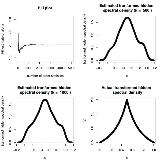
Figure 2. Hill plot of $\alpha^{(2)}$ and estimated and actual transformed hidden spectral densities

We test accuracy of our estimates of $\alpha^{(2)}$ and $\tilde{S}^{(2)}(\cdot)$. The Hill plot for $\{m^{(2)}_{i},i=1,2,\cdots,n\},$ the plot of the estimated transformed hidden spectral densities for $k=500,1000$, and the plot of the actual transformed hidden spectral density (7.3) are shown in Figure 2. We also estimate probabilities of risk sets of the form $P[X_{1}>t_{1},Y_{1}>t_{2}]$ for large thresholds $t_{1}$ and $t_{2}$. Using a method similar to the one used to obtain (6.10), we estimate the probability $P[X_{1}>t_{1},Y_{1}>t_{2}]$ as

$$P[X_{1}>t_{1},Y_{1}>t_{2}]\approx\frac{k}{n}\int_{\delta\aleph^{(2)}}{\Bigl{(}\Bigl{[}\frac{1}{\theta^{1}}{\Bigl{(}\frac{t_{1}}{X_{(\lceil 1/m^{(2)}_{(k)}\rceil)}}\Bigr{)}}^{\hat{\beta}^{1}}\Bigr{]}\bigvee\Bigl{[}\frac{1}{\theta^{2}}{\Bigr{(}\frac{t_{2}}{Y_{(\lceil 1/m^{(2)}_{(k)}\rceil)}}\Bigr{)}}^{\hat{\beta}^{2}}\Bigr{]}\Bigr{)}}^{-\hat{\alpha}^{(2)}}\hat{S}^{(2)}(d{\bf{\theta}}),$$

where $X_{(1)}\geq X_{(2)}\geq\cdots\geq X_{(n)}$ and $Y_{(1)}\geq Y_{(2)}\geq\cdots\geq Y_{(n)}$ are the order statistics for $\{X_{i},i=1,\cdots,n\}$ and $\{Y_{i},i=1,\cdots,n\}$, and the remaining notation has the same meaning as in (6.10). Since we simulate the data we take $\hat{\beta}_{1}=1$ and $\hat{\beta}_{2}=2$ and concentrate on estimating $\alpha^{(2)}$ using the Hill estimator and estimating $S^{(2)}$ by the formula given in (3.14). We compute the estimates of $P[X_{1}>100,Y_{1}>\sqrt{10}]$ for different values of $k$ using these estimators and plot the graph in Figure 3. The range of $k$ is $k=500$ to $k=5000.$

A different estimate of $P[X_{1}>t_{1},Y_{1}>t_{2}]$ is given by Heffernan and Resnick [15]:

$$P[X_{1}>t_{1},Y_{1}>t_{2}]\approx\frac{k}{n}\hat{\nu}^{(2)}\Bigl{(}\Bigl{(}\Bigl{(}{\Bigl{(}\frac{t_{1}}{X_{(\lceil 1/m^{(2)}_{(k)}\rceil)}}\Bigr{)}}^{\hat{\beta}^{1}},{\Bigl{(}\frac{t_{2}}{Y_{(\lceil 1/m^{(2)}_{(k)}\rceil)}}\Bigr{)}}^{\hat{\beta}^{2}}\Bigr{)},\boldsymbol{\infty}\Bigr{]}\Bigr{)},$$

where $\hat{\nu}^{(2)}$ is defined in (3.11). We again use $\hat{\beta}_{1}=1,\hskip 2.84544pt\hat{\beta}_{2}=2$ and estimate $\alpha^{(2)}$ using the Hill estimator. Then, using the above estimator, we compute the probability $P[X_{1}>100,Y_{1}>\sqrt{10}]$ for different values of $k$ and plot it as a graph in Figure 3. The values of $k$ are chosen between $k=500$ and $k=5000.$

Using the true distribution of $(X_{1},Y_{1}),$ we calculate $P[X_{1}>100,Y_{1}>\sqrt{10}]=0.001.$ In Figure 3, we observe that the plot of the risk estimates obtained using the Heffernan-Resnick [15] estimator is more stable but our current estimator of $P[X_{1}>100,Y_{1}>\sqrt{10}]$ is more accurate for most $k$ in the range $k=500$ to $k=5000$.

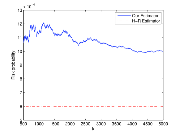
Figure 3. Plots of estimates of $P[X_{1}>100,Y_{1}>\sqrt{10}]$ for different values of k (sample size = 5000) using both our and H-R(Heffernan-Resnick [15]) estimator

The Heffernan-Resnick [15] estimator of $P[X_{1}>t_{1},Y_{1}>t_{2}]$ uses an empirical distribution function and thus is subject to the defect that a zero estimate is reported for the risk probability when $t_{1}$ and $t_{2}$ are high but actually $P[X_{1}>t_{1},Y_{1}>t_{2}]$ is non-zero. Irrespective of how high the threshold is, our estimator does not estimate $P[X_{1}>t_{1},Y_{1}>t_{2}]$ as zero, unless it is actually zero.

As an illustration, we reduced the sample size to $n=500$ and applied the two estimators of the risk probability $P[X_{1}>100,Y_{1}>\sqrt{10}]$. As suspected, the Heffernan-Resnick [15] estimator estimates the probability $P[X_{1}>100,Y_{1}>\sqrt{10}]$ as zero, whereas our estimator is still reasonably accurate. This is shown in Figure 4 where $k$ ranges between $k=50$ and $k=500.$

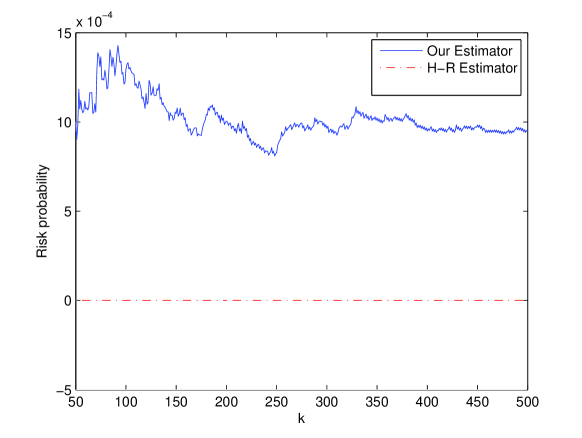
Figure 4. Plots of estimates of $P[X_{1}>100,Y_{1}>\sqrt{10}]$ for different values of k (sample size = 500) using both our and H-R(Heffernan-Resnick [15]) estimator

7.2. Internet traffic data

We analyze HTTP Internet response data consisting of sizes and durations of responses collected during a four hour period from 1–5 pm on April 26, 2001 by the University of North Carolina at Chapel Hill Department of Computer Science’s Distributed and Real-Time Systems Group under the direction of Don Smith and Kevin Jaffey. This dataset was also analyzed in [15]. We investigate joint behavior of two variables - size of response and throughput (size of response/time duration of response) and estimate the probability that both the size and rate are big as a measure of burstiness.

We start by estimating marginal tail parameters. We use QQ plots [28, page 97] (not shown here) to choose the value $k=5000$ for both the variables size and rate. Using this $k$, we get the estimates of tail indices $\hat{\beta}^{1}=1.15$ and $\hat{\beta}^{2}=1.51$ for size and rate using the QQ estimator.

Next, we investigate presence of asymptotic independence by plotting an estimated density of the transformed spectral measure $\tilde{S}(\cdot),$ defined in Section 4.1. In agreement with Heffernan and Resnick [15], our estimated density plots for different values of $k$ for the transformed spectral measure show two modes at the points $0$ and $1$ and take values close to zero in between, thus indicating asymptotic independence of size and rate (plots are not shown).

Is hidden regular variation present? The Hill plot in Figure 5 of $\{m^{(2)}_{i},1\leq i\leq n\}$ suggests this is so and we proceed to estimate the density of the transformed hidden spectral measure. Figure 5 gives plots of the estimated transformed hidden spectral densities for $k=500,1000,5000$.

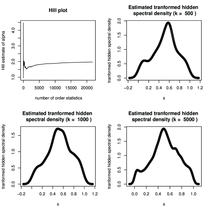
Figure 5. Hill plot of $\alpha^{(2)}$ and estimated transformed hidden spectral densities

Next, we estimate probabilities of risk sets of the form $[\text{Size}>x,\text{Rate}>y]$ which we consider as measures of burstiness. Examination of the (Size, Rate) data, indicates $x=2\times 10^{7}$ and $y=10^{5}$ are reasonably high thresholds. We use both our estimator and the estimator given in [15] to compute $P[\text{Size}>x,\text{Rate}>y]$ for different values of $k$ from $k=500$ to $k=n$ and plot them in Figure 6.

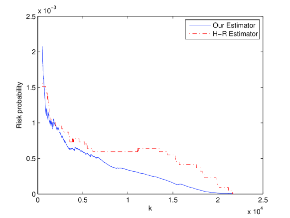
Figure 6. Plots of estimates of $P[\text{Size}>2\times 10^{7},\text{Rate}>10^{5}]$ for different values of $k$ using our estimator and H-R(Heffernan-Resnick [15]) estimator

We also estimated $P[\text{Size}>x,\text{Rate}>y]$ for higher thresholds $x=2\times 10^{8}$ and $y=10^{7},$ as a measure of extreme traffic burstiness. Again, we use both our estimator and the Heffernan-Resnick [15] estimator to estimate $P[\text{Size}>x,\text{Rate}>y]$ for different values of $k$ from $k=500$ to $k=n$ and plot them in Figure 7. If hidden regular variation is present for the pair (Size, Rate), then the actual risk probability cannot be zero. The Heffernan-Resnick [15] estimator reports an estimate of zero but ours does not.

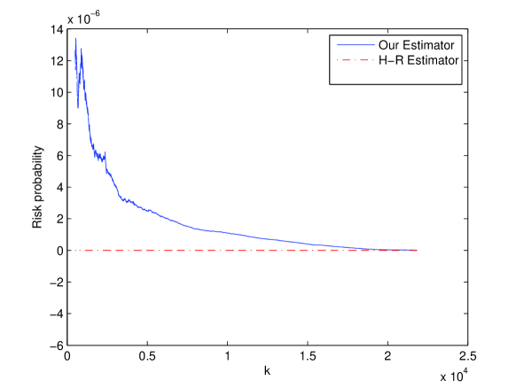
Figure 7. Plots of estimates of $P[\text{Size}>2\times 10^{8},\text{Rate}>10^{6}]$ for different values of $k$ using our estimator and H-R( Heffernan-Resnick [15]) estimator

8. Concluding remarks

Hidden regular variation provides a sub-family of the distributions having regular variation on $\operatorname{\mathbb{E}}$ that is sometimes equipped to obtain more precise estimates of probabilities of certain risk sets, which are crudely estimated as zero by regular variation on $\operatorname{\mathbb{E}}$; two examples are shown in Section 6.

The theory of HRV has deficiencies. Consider $d=3$, and on the planes of $\operatorname{\mathbb{E}}^{(2)}$, suppose the random vector ${\bf{Z}}$ has regular variation with three different tail indices $\alpha^{(2),1}<\alpha^{(2),2}<\alpha^{(2),3}$. As a convention, say ${\bf{Z}}$ has regular variation with tail index $\alpha^{(2),i}$ on $\{{\bf{x}}\in\operatorname{\mathbb{E}}^{(2)}:x^{i}=0\}$, $i=1,2,3$. If we follow our HRV model and method of estimation, we ignore the regular variation ${\bf{Z}}$ exhibits on $\{{\bf{x}}\in\operatorname{\mathbb{E}}^{(2)}:x^{2}=0\}$ with tail index $\alpha^{(2),2}$, which is actually more important than the regular variation on $\operatorname{\mathbb{E}}^{(3)}$. A way to repair this defect is the following alternative method: In $d$ dimensions, first consider the big cone $\operatorname{\mathbb{E}}$, then consider all the $d\choose 2$ pairs of components of ${\bf{Z}}$ and their regular variation on $(0,\infty]^{2}$, then consider all the $d\choose 3$ triplets of components of ${\bf{Z}}$ and their regular variation on $(0,\infty]^{3}$, and so on. This alternative method requires considering regular variation on $2^{d}-1$ cones, whereas our HRV formulation requires considering regular variation on at most $d$ cones. The alternative method is difficult to apply in high dimensions. Obviously, there is considerable flexibility in choosing a nested sequence of cones and informed choice by a practicioner will be governed by the application.

Another potential defect of our formulation of HRV is that it is designed to deal with the kind of degeneracy which arises when the limit measures are concentrated on the axes, planes etc. But the limit measures might exhibit different kind of degeneracies. For example, consider the degeneracy in the case of complete asymptotic dependence, where the limit measure is concentrated on the ray $\{{\bf{x}}\in\operatorname{\mathbb{E}}:x^{1}=x^{2}=\cdots=x^{d}\}$. One might think of removing the ray and considering hidden regular variation on the cone $\operatorname{\mathbb{E}}\setminus\{{\bf{x}}\in\operatorname{\mathbb{E}}:x^{1}=x^{2}=\cdots=x^{d}\}$. Our HRV discussion does not address this issue and we are currently actively thinking about this as well as methods of unifying theories of HRV and the conditional extreme value model [17, 16, 7, 6, 14, 13].

Other variants of our formulation are possible. The hidden variation on a subcone could be of extreme value type other than regular variation and even if we focus only on the hidden variation being regular variation, one could envisage different scaling functions for the hidden variation. These topics are also being actively considered.

In estimating the limit measure $\nu^{(l)}$ of hidden regular variation on $\operatorname{\mathbb{E}}^{(l)}$, $2\leq l\leq d$, we have suggested a method that exploits the semi-parametric structure of $\nu^{(l)}$. Also, we have constructed a consistent estimator of $\nu^{(l)}$ which relies completely on non-parametric methods, as given in (3.10). Our numerical experiments in Section 7 clearly suggest the method exploiting the semi-parametric structure is superior, presumably because it uses more available information about the limit measure $\nu^{(l)}$. However, we have no precise, provable comparison.

An important statistical issue is we have only developed parameter estimators which are consistent. We have not yet developed theory which allows one to report on confidence intervals for parameter estimates or risk probability estimates.

For characterizations of hidden regular variation, it is important to identify when $\nu^{(l)}(\{{\bf{x}}\in\operatorname{\mathbb{E}}^{(l)}:||{\bf{x}}||>1\})$ is finite. We found a moment condition to check this, but it requires knowledge of the hidden angular measure $S^{(l)}$. A similar problem appeared in checking the finiteness of the right side of (6.2). It would be useful to have a statistical test for finiteness.

9. Acknowledgements

S. I. Resnick and A. Mitra were partially supported by ARO Contract W911NF-07-1-0078 at Cornell University.

Appendix A

Proof of Proposition 3.1.

The idea of the proof is similar to Proposition 2 of [26]. Define $\operatorname{\mathbb{E}}_{l\setminus\infty}=\operatorname{\mathbb{E}}^{(l)}\backslash\cup_{1\leq i_{1}<i_{2}<\cdots i_{l}\leq d}[x^{i_{1}}=\infty,x^{i_{2}}=\infty,\cdots,x^{i_{l}}=\infty]$ and $\operatorname{\mathbb{E}}_{2}=(0,\infty)\times\delta\aleph^{(l)}.$ Define a continuous bijection $Q^{(l)}:\operatorname{\mathbb{E}}_{l\setminus\infty}\to\operatorname{\mathbb{E}}_{2}$ as in (3.4). We first show the equivalence of the vague convergence of measures restricted to $\operatorname{\mathbb{E}}_{l\setminus\infty}$ and $\operatorname{\mathbb{E}}_{2}$, and then extend the convergence to the corresponding whole spaces using the scaling property.
Step 1: First, we prove the direct part. So, we suppose that (2.10) holds with $\nu^{(l)}(\aleph^{(l)})=1$. Hence, the convergence also holds with the measures being restricted to $\operatorname{\mathbb{E}}_{l\setminus\infty}$, i.e.

$$tP\left[\frac{{\bf{Z}}}{b^{(l)}(t)}\in\cdot\cap\operatorname{\mathbb{E}}_{l\setminus\infty}\right]\stackrel{{\scriptstyle v}}{{\rightarrow}}\nu^{(l)}(\cdot\cap\operatorname{\mathbb{E}}_{l\setminus\infty})\quad\text{in $M_{+}(\operatorname{\mathbb{E}}_{l\setminus\infty})$}.$$

Now, we proceed to show that for each compact set $K_{2}$ in $\operatorname{\mathbb{E}}_{2}$, ${(Q^{(l)})}^{-1}(K_{2})$ is a compact set of $\operatorname{\mathbb{E}}_{l\setminus\infty}$. Note that the compact sets in $\operatorname{\mathbb{E}}_{l\setminus\infty}$ are those closed sets $K$ for which every ${\bf{x}}\in K$ satisfies the property that $r\leq x^{(l)}\leq s$ for some $0<r<s$ [28, page 170]. Take a compact set $K_{2}$ in $\operatorname{\mathbb{E}}_{2}$. We claim that $K_{2}$ must be contained in a set $\tilde{K}_{2}$ of the form $\tilde{K}_{2}=[r,s]\times\delta\aleph^{(l)}$. Now, from the description of the compact sets of $\operatorname{\mathbb{E}}_{l\setminus\infty}$, ${(Q^{(l)})}^{-1}(\tilde{K}_{2})=\{{\bf{x}}\in\operatorname{\mathbb{E}}^{(l)}:r\leq x^{(l)}\leq s\}$ is compact in $\operatorname{\mathbb{E}}_{l\setminus\infty}$. Also, since $Q^{(l)}$ is continuous, ${(Q^{(l)})}^{-1}(K_{2})$ is closed. Therefore, ${(Q^{(l)})}^{-1}(K_{2})$ is a closed subset of the compact set ${(Q^{(l)})}^{-1}(\tilde{K}_{2})$ and hence is compact in $\operatorname{\mathbb{E}}_{l\setminus\infty}$. So, using Proposition 5.5 (b) of [28] we get

$$tP\left[\left(\frac{Z^{(l)}}{b^{(l)}(t)},\frac{{\bf{Z}}}{Z^{(l)}}\right)\in\cdot\cap\operatorname{\mathbb{E}}_{2}\right]\stackrel{{\scriptstyle v}}{{\rightarrow}}\nu_{\alpha^{(l)}}\times S^{(l)}(\cdot\cap\operatorname{\mathbb{E}}_{2})\quad\text{in $M_{+}(\operatorname{\mathbb{E}}_{2})$}.$$

Now, we want to extend the convergence over the whole space $(0,\infty]\times\delta\aleph^{(l)}.$ Choose any relatively compact subset $\Lambda$ of $\delta\aleph^{(l)}$ such that $S^{(l)}(\delta\Lambda)=0$ and choose $s>r>0$. Then,

$$tP\left[\frac{Z^{(l)}}{b^{(l)}(t)}>r,\frac{{\bf{Z}}}{Z^{(l)}}\in\Lambda\right] \geq tP\left[\frac{Z^{(l)}}{b^{(l)}(t)}\in(r,s],\frac{{\bf{Z}}}{Z^{(l)}}\in\Lambda\right]\to\nu_{\alpha^{(l)}}((r,s])S^{(l)}(\Lambda)$$

as $$t\to\infty, s>r>0$$ which implies that for ,

$$\liminf_{t\to\infty}tP \left[\frac{Z^{(l)}}{b^{(l)}(t)}>r,\frac{{\bf{Z}}}{Z^{(l)}}\in\Lambda\right]\geq\nu_{\alpha^{(l)}}((r,s])S^{(l)}(\Lambda).$$

Hence, letting $$s\to\infty$$, we get

(A.1) $$\liminf_{t\to\infty}tP \left[\frac{Z^{(l)}}{b^{(l)}(t)}>r,\frac{{\bf{Z}}}{Z^{(l)}}\in\Lambda\right]\geq r^{-\alpha^{(l)}}S^{(l)}(\Lambda).$$

Now, we know that

(A.2) $$tP\left[\frac{Z^{(l)}}{b^{(l)}(t)}>r,\frac{{\bf{Z}}}{Z^{(l)}}\in\Lambda\right]=tP\left[\frac{Z^{(l)}}{b^{(l)}(t)}\in(r,s],\frac{{\bf{Z}}}{Z^{(l)}}\in\Lambda\right]+tP\left[\frac{Z^{(l)}}{b^{(l)}(t)}>s,\frac{{\bf{Z}}}{Z^{(l)}}\in\Lambda\right],$$

and

$$\lim_{s\to\infty}\limsup_{t\to\infty} tP\left[\frac{Z^{(l)}}{b^{(l)}(t)}>s,\frac{{\bf{Z}}}{Z^{(l)}}\in\Lambda\right]\leq\lim_{s\to\infty}\limsup_{t\to\infty}tP\left[\frac{Z^{(l)}}{b^{(l)}(t)}>s\right]$$

(A.3) $$=\lim_{s\to\infty}\nu^{(l)}(\{{\bf{x}}\in\operatorname{\mathbb{E}}^{(l)}:x^{(l)}>s\})=\lim_{s\to\infty}s^{-\alpha^{(l)}}\nu^{(l)}(\{{\bf{x}}\in\operatorname{\mathbb{E}}^{(l)}:x^{(l)}>1\})=0.$$

The first equality in the above set of relations follows from (2.10). Hence, from (A.2) and (A), we get

(A.4) $$\limsup_{t\to\infty}tP\left[\frac{Z^{(l)}}{b^{(l)}(t)}>r,\frac{{\bf{Z}}}{Z^{(l)}}\in\Lambda\right]\leq\lim_{s\to\infty}\limsup_{t\to\infty}tP\left[\frac{Z^{(l)}}{b^{(l)}(t)}\in(r,s],\frac{{\bf{Z}}}{Z^{(l)}}\in\Lambda\right]=r^{-\alpha^{(l)}}S^{(l)}(\Lambda).$$

Hence, from (A) and (A.4), we conclude the direct part of the proof:

$$\lim_{t\to\infty}tP\left[\frac{Z^{(l)}}{b^{(l)}(t)}>r,\frac{{\bf{Z}}}{Z^{(l)}}\in\Lambda\right]=r^{-\alpha^{(l)}}S^{(l)}(\Lambda).$$

Step 2: To see the converse, again we prove first the vague convergence of the restricted measures in $M_{+}(\operatorname{\mathbb{E}}_{l\setminus\infty})$ and then extend it to convergence of measures in $M_{+}(\operatorname{\mathbb{E}}^{(l)})$. We assume that (3.1) holds. Restriction on $\operatorname{\mathbb{E}}_{2}$ gives

$$tP\left[\left(\frac{Z^{(l)}}{b^{(l)}(t)},\frac{{\bf{Z}}}{Z^{(l)}}\right)\in\cdot\cap\operatorname{\mathbb{E}}_{2}\right]\stackrel{{\scriptstyle v}}{{\rightarrow}}\nu_{\alpha^{(l)}}\times S^{(l)}(\cdot\cap\operatorname{\mathbb{E}}_{2})\quad\text{in $M_{+}(\operatorname{\mathbb{E}}_{2})$}.$$

First we note that the compact sets of $\operatorname{\mathbb{E}}_{2}$ are those closed sets $K$ for which every $(w,{\bf{v}})\in K$ satisfies the property that $r\leq w\leq s$ for some $0<r<s.$ Take a compact set $K_{1}$ of $\operatorname{\mathbb{E}}_{l\setminus\infty}$. Observe, from the description of the compact sets of $\operatorname{\mathbb{E}}_{l\setminus\infty}$ as given before, that $K_{1}$ must be contained in a set $\tilde{K}_{1}$ of the form $\tilde{K}_{1}=\{{\bf{x}}\in\operatorname{\mathbb{E}}^{(l)}:x^{(l)}\in[r,s]\}$. From the description of compact sets of $\operatorname{\mathbb{E}}_{2}$, $Q^{(l)}(\tilde{K}_{1})=[r,s]\times\delta\aleph^{(l)}$ is compact in $\operatorname{\mathbb{E}}_{2}$. Since ${(Q^{(l)})}^{-1}$ is also continuous, the set $Q^{(l)}(K_{1})$ is closed, and hence, being a closed subset of a compact set $Q^{(l)}(\tilde{K}_{1})$, is compact. Therefore, using the continuous map ${(Q^{(l)})}^{-1}:\operatorname{\mathbb{E}}_{2}\to\operatorname{\mathbb{E}}_{l\setminus\infty}$ and Proposition 5.5 (b) of [28], we get

$$tP\left[\frac{{\bf{Z}}}{b^{(l)}(t)}\in\cdot\cap\operatorname{\mathbb{E}}_{l\setminus\infty}\right]\stackrel{{\scriptstyle v}}{{\rightarrow}}\nu^{(l)}(\cdot\cap\operatorname{\mathbb{E}}_{l\setminus\infty})\quad\text{in $M_{+}(\operatorname{\mathbb{E}}_{l\setminus\infty})$}.$$

Now, we want to extend this convergence over the whole space $\operatorname{\mathbb{E}}^{(l)}$. Choose a relatively compact set $A$ of $\operatorname{\mathbb{E}}^{(l)}$ such that $\nu^{(l)}(\delta A)=0$. Note that, from the description of relatively compact sets in $\operatorname{\mathbb{E}}^{(l)}$ as given in Section 2.2.2, $A\subseteq\{{\bf{x}}\in\operatorname{\mathbb{E}}^{(l)}:x^{(l)}>r\}$ for some $r>0$. Also, from the earlier description of compact sets of $\operatorname{\mathbb{E}}_{l\setminus\infty}$, it follows that for all $s>r$, $A\cap\{{\bf{x}}\in\operatorname{\mathbb{E}}^{(l)}:x^{(l)}<s\}$ is a relatively compact set of $\operatorname{\mathbb{E}}_{l\setminus\infty}$, and

$$\nu^{(l)}(\delta(A\cap\{{\bf{x}}\in\operatorname{\mathbb{E}}^{(l)}:x^{(l)}<s\}))\leq\nu^{(l)}(\delta A)+\nu^{(l)}(\{{\bf{x}}\in\operatorname{\mathbb{E}}^{(l)}:x^{(l)}=s\})=0.$$

Hence, it follows that

$$tP\left[\frac{{\bf{Z}}}{b^{(l)}(t)}\in A\right]\geq tP \left[\frac{{\bf{Z}}}{b^{(l)}(t)}\in A\cap\{{\bf{x}}\in\operatorname{\mathbb{E}}^{(l)}:x^{(l)}<s\}\right]\to\nu^{(l)}(A\cap\{{\bf{x}}\in\operatorname{\mathbb{E}}^{(l)}:x^{(l)}<s\}),$$

which implies, by letting $s\to\infty$,

(A.5) $$\liminf_{t\to\infty}tP \left[\frac{{\bf{Z}}}{b^{(l)}(t)}\in A\right]\geq\nu^{(l)}(A),$$

since by (2.11), $\nu^{(l)}(\{{\bf{x}}\in\operatorname{\mathbb{E}}^{(l)}:x^{(l)}=\infty\})=0$. Now, we know that

(A.6) $$tP\left[\frac{{\bf{Z}}}{b^{(l)}(t)}\in A\right]=tP \left[\frac{{\bf{Z}}}{b^{(l)}(t)}\in A\cap\{{\bf{x}}\in\operatorname{\mathbb{E}}^{(l)}:x^{(l)}<s\}\right]+tP\left[\frac{{\bf{Z}}}{b^{(l)}(t)}\in A\cap\{{\bf{x}}\in\operatorname{\mathbb{E}}^{(l)}:x^{(l)}\geq s\}\right],$$

and

$$\lim_{s\to\infty}\limsup_{t\to\infty} tP\left[\frac{{\bf{Z}}}{b^{(l)}(t)}\in A\cap\{{\bf{x}}\in\operatorname{\mathbb{E}}^{(l)}:x^{(l)}\geq s\}\right]\leq\lim_{s\to\infty}\limsup_{t\to\infty}tP\left[\frac{{\bf{Z}}}{b^{(l)}(t)}\in\{{\bf{x}}\in\operatorname{\mathbb{E}}^{(l)}:x^{(l)}\geq s\}\right]$$

(A.7) $$=\lim_{s\to\infty}\limsup_{t\to\infty}tP\left[\frac{Z^{(l)}}{b^{(l)}(t)}\geq s\right]=\lim_{s\to\infty}\nu_{\alpha^{(l)}}([s,\infty])=\lim_{s\to\infty}s^{-\alpha^{(l)}}=0.$$

The second equality in the above set of relations follows from (3.1). Hence, from (A.6) and (A), we get

(A.8) $$\limsup_{t\to\infty}tP\left[\frac{{\bf{Z}}}{b^{(l)}(t)}\in A\right]\leq\lim_{s\to\infty}\limsup_{t\to\infty}tP\left[\frac{{\bf{Z}}}{b^{(l)}(t)}\in A\cap\{{\bf{x}}\in\operatorname{\mathbb{E}}^{(l)}:x^{(l)}<l\}\right]=\nu^{(l)}(A).$$

Therefore, from (A.5) and (A.8), we conclude

$$\lim_{t\to\infty}tP\left[\frac{{\bf{Z}}}{b^{(l)}(t)}\in A\right]=\nu^{(l)}(A),$$

which completes the converse part of the proof.

∎

Appendix B

Proof of Proposition 3.7.

The idea of this proof is similar to Theorem 6.1 of [28, page 173]. Define, $\operatorname{\mathbb{E}}_{l\setminus\infty}=\operatorname{\mathbb{E}}^{(l)}\backslash\cup_{1\leq i_{1}<i_{2}<\cdots<i_{l}\leq d}[x^{i_{1}}=\infty,x^{i_{2}}=\infty,\cdots,x^{i_{l}}=\infty]$ and $\operatorname{\mathbb{E}}_{2}=(0,\infty)\times\delta\aleph^{(l)}$. Now, define the continuous bijection $Q^{(l)}:\operatorname{\mathbb{E}}_{l\setminus\infty}\to\operatorname{\mathbb{E}}_{2}$ as in (3.4). As in Proposition 3.1, here also the idea of the proof is to first show the equivalence of the weak convergence of random measures restricted to $M_{+}(\operatorname{\mathbb{E}}_{l\setminus\infty})$ and $M_{+}(\operatorname{\mathbb{E}}_{2})$, and then extend the convergence to the corresponding whole spaces using the scaling property.

Step 1: First, we prove that (3.11) implies (3.12). The convergence in (3.11) implies

$$\hat{\nu}^{(l)}(\cdot\cap\operatorname{\mathbb{E}}_{l\setminus\infty}):=\frac{1}{k}\sum_{i=1}^{n}\epsilon_{\left((1/r_{i}^{j})/m^{(l)}_{(k)},1\leq j\leq d\right)}1_{\{m^{(l)}_{i}/m^{(l)}_{(k)}<\infty\}}\Rightarrow\nu^{(l)}(\cdot\cap\operatorname{\mathbb{E}}_{l\setminus\infty})$$

on $M_{+}(\operatorname{\mathbb{E}}_{l\setminus\infty})$. Also, as shown in the proof of Proposition 3.1, for any compact set $K_{2}\subset\operatorname{\mathbb{E}}_{2}$, ${(Q^{(l)})}^{-1}(K_{2})$ is compact in $\operatorname{\mathbb{E}}_{l\setminus\infty}$. Then, using Proposition 5.5(b) of [28] we get

(B.1) $$\hat{\nu}^{(l)}(\cdot\cap\operatorname{\mathbb{E}}_{l\setminus\infty})\circ{(Q^{(l)})}^{-1}:=\frac{1}{k}\sum_{i=1}^{n}\epsilon_{\left(m^{(l)}_{i}/m^{(l)}_{(k)},\hskip 5.69046pt\left((1/r_{i}^{j})/m^{(l)}_{i},\hskip 2.84544pt1\leq j\leq d\right)\right)}1_{\{m^{(l)}_{i}/m^{(l)}_{(k)}<\infty\}}\Rightarrow\nu_{\alpha^{(l)}}\times S^{(l)}(\cdot\cap\operatorname{\mathbb{E}}_{2})$$

on $M_{+}(\operatorname{\mathbb{E}}_{2})$. To extend the convergence to the space $(0,\infty]\times\delta\aleph^{(l)}$, we use the convergence of laplace functionals and use Theorem 5.2 of [28, page 137]. Take $f\in C_{K}^{+}((0,\infty]\times\delta\aleph^{(l)})$, where $C_{K}^{+}(\mathbb{F})$ is the set of all continuous functions with compact support from $\mathbb{F}$ to $\mathbb{R}^{+}$. To relate this function to one defined in $C_{K}^{+}((0,\infty)\times\delta\aleph^{(l)})$, for all $\delta,M>0$, we define a truncation function

$$\phi_{\delta,M}=\left\{\begin{array}[]{cc}1&\hbox{if}\hskip 2.84544pt0<t\leq M\\ 0&\hbox{if}\hskip 2.84544ptt>M+\delta,\\ \hbox{linear interpolation}&\hbox{if}\hskip 2.84544ptM<t\leq M+\delta.\end{array}\right.$$

Note that $f_{\delta,M}(r,\theta):=f(r,\theta)\phi_{\delta,M}(r)\in C_{K}^{+}((0,\infty)\times\delta\aleph^{(l)})$ for all $\delta,M>0$. Note that

$$|E \left[\exp\left[-\frac{1}{k}\sum_{i=1}^{n}f\left(m^{(l)}_{i}/m^{(l)}_{(k)},\hskip 2.84544pt\left((1/r_{i}^{j})/m^{(l)}_{i},\hskip 2.84544pt1\leq j\leq d\right)\right)\right]\right]-\exp\left[-\nu_{\alpha^{(l)}}\times S^{(l)}(f)\right]|$$

$$\leq|E\left[\exp\left[-\frac{1}{k}\sum_{i=1}^{n}f\left(m^{(l)}_{i}/m^{(l)}_{(k)},\hskip 5.69046pt\left((1/r_{i}^{j})/m^{(l)}_{i},\hskip 2.84544pt1\leq j\leq d\right)\right)\right]\right]$$

$$\qquad-E\left[\exp\left[-\frac{1}{k}\sum_{i=1}^{n}f_{\delta,M}\left(m^{(l)}_{i}/m^{(l)}_{(k)},\hskip 5.69046pt\left((1/r_{i}^{j})/m^{(l)}_{i},\hskip 2.84544pt1\leq j\leq d\right)\right)\right]\right]|$$

$$+ |E\left[\exp\left[-\frac{1}{k}\sum_{i=1}^{n}f_{\delta,M}\left(m^{(l)}_{i}/m^{(l)}_{(k)},\hskip 5.69046pt\left((1/r_{i}^{j})/m^{(l)}_{i},\hskip 2.84544pt1\leq j\leq d\right)\right)\right]\right]-\exp\left[-\nu_{\alpha^{(l)}}\times S^{(l)}(f_{\delta,M})\right]|$$

$$+|\exp\left[-\nu_{\alpha^{(l)}}\times S^{(l)}(f_{\delta,M})\right]-\exp\left[-\nu_{\alpha^{(l)}}\times S^{(l)}(f)\right]|$$

$$\qquad=A+B+C.$$

Since, $f_{\delta,M}\in C_{K}^{+}((0,\infty)\times\delta\aleph^{(l)})$, by (B.1), we get $\lim_{n\to\infty}B=0$. Now, we proceed to show that $\lim_{M\to\infty}\limsup_{n\to\infty}A=0$. Notice that

$$\limsup_{n\to\infty}|E \left[\exp\left[-\frac{1}{k}\sum_{i=1}^{n}f\left(m^{(l)}_{i}/m^{(l)}_{(k)},\hskip 5.69046pt\left((1/r_{i}^{j})/m^{(l)}_{i},\hskip 2.84544pt1\leq j\leq d\right)\right)\right]\right]$$

$$\qquad-E\left[\exp\left[-\frac{1}{k}\sum_{i=1}^{n}f_{\delta,M}\left(m^{(l)}_{i}/m^{(l)}_{(k)},\hskip 5.69046pt\left((1/r_{i}^{j})/m^{(l)}_{i},\hskip 2.84544pt1\leq j\leq d\right)\right)\right]\right]|$$

$$=\limsup_{n\to\infty}E\left[\exp\left[-\frac{1}{k}\sum_{i=1}^{n}f\left(m^{(l)}_{i}/m^{(l)}_{(k)},\hskip 5.69046pt\left((1/r_{i}^{j})/m^{(l)}_{i},\hskip 2.84544pt1\leq j\leq d\right)\right)\right]\right.$$

$$\hskip 28.45274pt\times\left.\left(1-\exp\left[-\frac{1}{k}\sum_{i=1}^{n}(f_{\delta,M}-f)\left(m^{(l)}_{i}/m^{(l)}_{(k)},\hskip 5.69046pt\left((1/r_{i}^{j})/m^{(l)}_{i},\hskip 2.84544pt1\leq j\leq d\right)\right)\right]\right)\right]$$

$$\leq\limsup_{n\to\infty}E\left[\left(1-\exp\left[-\frac{1}{k}\sum_{i=1}^{n}(f_{\delta,M}-f)\left(m^{(l)}_{i}/m^{(l)}_{(k)},\hskip 5.69046pt\left((1/r_{i}^{j})/m^{(l)}_{i},\hskip 2.84544pt1\leq j\leq d\right)\right)\right]\right)\right],$$

which, using the facts that $$||f||=\sup_{(r,\theta)\in(0,\infty]\times\delta\aleph^{(l)}}f(r,\theta)<\infty ||f_{\delta,M}-f||\leq||f||\cdot||\phi_{\delta,M}-1||\leq||f|| (f_{\delta,M}-f)(x,{\bf{\theta}})=0 x<M$$, and for , is bounded by

$$\limsup_{n\to\infty}E\left[1-\exp\left[-\frac{1}{k}||f||\sum_{i=1}^{n}\epsilon_{m^{(l)}_{i}/m^{(l)}_{(k)}}([M,\infty])\right]\right]$$

$$=E\left[1-\exp\left[-||f||\frac{1}{k}\sum_{i=1}^{n}\epsilon_{\left((1/r_{i}^{j})/m^{(l)}_{(k)},1\leq j\leq d\right)}(\{{\bf{x}}\in\operatorname{\mathbb{E}}^{(l)}:x^{(l)}\in[M,\infty]\})\right]\right],$$

which, by (3.11), converges as $$n\to\infty$$, to

$$1-\exp\left[-||f||\cdot\nu^{(l)}(\{{\bf{x}}\in\operatorname{\mathbb{E}}^{(l)}:x^{(l)}\in[M,\infty]\})\right]$$

$$=1-\exp\left[-||f||\cdot M^{-\alpha^{(l)}}\nu^{(l)}(\aleph^{(l)})\right]$$

$$=1-\exp\left[-||f||\cdot M^{-\alpha^{(l)}}\right]\rightarrow 0,$$

as $M\to\infty$. The argument for $\lim_{M\to\infty}C=0$ is similar and is omitted. Hence, by Theorem 5.2 of [28, page 137], we obtain (3.12).

Step 2: To see the other part, i.e. (3.12) implies (3.11), we use a similar method. The convergence in (3.12) implies

$$\frac{1}{k}\sum_{i=1}^{n}\epsilon_{\left(\left(m^{(l)}_{i}/m^{(l)}_{(k)},\hskip 2.84544pt(1/r_{i}^{j})/m^{(l)}_{i}\right),\hskip 2.84544pt1\leq j\leq d\right)}((\cdot)\cap\operatorname{\mathbb{E}}_{2})\Rightarrow\nu_{\alpha^{(l)}}\times S^{(l)}((\cdot)\cap\operatorname{\mathbb{E}}_{2})$$

on $M_{+}(\operatorname{\mathbb{E}}_{2})$. It is easy to see that ${(Q^{(l)})}^{-1}$ is a continuous bijection. Also, as shown in the proof of Proposition 3.1, for any compact set $K_{1}\subset\operatorname{\mathbb{E}}_{l\setminus\infty}$, $Q^{(l)}(K_{1})$ is compact in $\operatorname{\mathbb{E}}_{2}$. Therefore, using Proposition 5.5(b) of [28] we get

(B.2) $$\hat{\nu}^{(l)}((\cdot)\cap\operatorname{\mathbb{E}}_{l\setminus\infty}):=\frac{1}{k}\sum_{i=1}^{n}\epsilon_{\left((1/r_{i}^{j})/m^{(l)}_{(k)},1\leq j\leq d\right)}1_{\{m_{i}^{(l)}/m_{(k)}^{(l)}<\infty\}}\Rightarrow\nu^{(l)}((\cdot)\cap\operatorname{\mathbb{E}}_{l\setminus\infty})$$

on $M_{+}(\operatorname{\mathbb{E}}_{l\setminus\infty})$. We use the same truncation function $\phi_{\delta,M}$ to relate functions on $C_{K}^{+}(\operatorname{\mathbb{E}}^{(l)})$ to ones in $C_{K}^{+}(\operatorname{\mathbb{E}}_{l\setminus\infty})$. Choose $f\in C_{K}^{+}(\operatorname{\mathbb{E}}^{(l)})$. Note that $f_{\delta,M}({\bf{x}}):=f({\bf{x}})\phi_{\delta,M}(x^{(l)})\in C_{K}^{+}(\operatorname{\mathbb{E}}_{l\setminus\infty})$ for all $\delta,M>0$.

$$| E\left[\exp\left[-\frac{1}{k}\sum_{i=1}^{n}f\left((1/r_{i}^{j})/m^{(l)}_{(k)},\hskip 2.84544pt1\leq j\leq d\right)\right]\right]-\exp\left[-\nu^{(l)}(f)\right]|$$

$$\leq|E\left[\exp\left[-\frac{1}{k}\sum_{i=1}^{n}f\left((1/r_{i}^{j})/m^{(l)}_{i},\hskip 2.84544pt1\leq j\leq d\right)\right]-\exp\left[-\frac{1}{k}\sum_{i=1}^{n}f_{\delta,M}\left((1/r_{i}^{j})/m^{(l)}_{i},\hskip 2.84544pt1\leq j\leq d\right)\right]\right]|$$

$$+|E\left[\exp\left[-\frac{1}{k}\sum_{i=1}^{n}f_{\delta,M}\left((1/r_{i}^{j})/m^{(l)}_{i},\hskip 2.84544pt1\leq j\leq d\right)\right]\right]-\exp\left[-\nu^{(l)}(f_{\delta,M})\right]|$$

$$\qquad+|\exp\left[-\nu^{(l)}(f_{\delta,M})\right]-\exp\left[-\nu^{(l)}(f)\right]|$$

$$\qquad=A+B+C.$$

Since, $f_{\delta,M}\in C_{K}^{+}(\operatorname{\mathbb{E}}_{l\setminus\infty})$, by (B.2), we get $\lim_{n\to\infty}B=0$. Now, we will show that $\lim_{M\to\infty}\limsup_{n\to\infty}A=0$.

$$\limsup_{n\to\infty}|E \left[\exp\left[-\frac{1}{k}\sum_{i=1}^{n}f\left((1/r_{i}^{j})/m^{(l)}_{i},\hskip 2.84544pt1\leq j\leq d\right)\right]-\exp\left[-\frac{1}{k}\sum_{i=1}^{n}f_{\delta,M}\left((1/r_{i}^{j})/m^{(l)}_{i},\hskip 2.84544pt1\leq j\leq d\right)\right]\right]|$$

$$=\limsup_{n\to\infty}E\left[\exp\left[-\frac{1}{k}\sum_{i=1}^{n}f\left((1/r_{i}^{j})/m^{(l)}_{i},\hskip 2.84544pt1\leq j\leq d\right)\right]\right.$$

$$\hskip 28.45274pt\times\left.\left(1-\exp\left[-\frac{1}{k}\sum_{i=1}^{n}(f_{\delta,M}-f)\left((1/r_{i}^{j})/m^{(l)}_{i},\hskip 2.84544pt1\leq j\leq d\right)\right]\right)\right]$$

$$\leq\limsup_{n\to\infty}E\left[\left(1-\exp\left[-\frac{1}{k}\sum_{i=1}^{n}(f_{\delta,M}-f)\left((1/r_{i}^{j})/m^{(l)}_{i},\hskip 2.84544pt1\leq j\leq d\right)\right]\right)\right],$$

which, using the facts $$||f||=\sup_{{\bf{x}}\in\operatorname{\mathbb{E}}^{(l)}}f({\bf{x}})<\infty ||f_{\delta,M}-f||\leq||f||\cdot||\phi_{\delta,M}-1||\leq||f|| (f_{\delta,M}-f)({\bf{x}})=0 \{{\bf{x}}\in\operatorname{\mathbb{E}}^{(l)}:x^{(l)}<M\}$$, and for , is bounded by

$$E\left[1-\exp\left[-\frac{1}{k}||f||\sum_{i=1}^{n}\epsilon_{\left((1/r_{i}^{j})/m^{(l)}_{(k)},1\leq j\leq d\right)}(\{{\bf{x}}\in\operatorname{\mathbb{E}}^{(l)}:x^{(l)}\in[M,\infty]\})\right]\right]$$

$$=\limsup_{n\to\infty}E\left[1-\exp\left[-||f||\frac{1}{k}\sum_{i=1}^{n}\epsilon_{m^{(l)}_{i}/m^{(l)}_{(k)}}([M,\infty])\right]\right],$$

which, by (3.12), converges as $$n\to\infty$$, to

$$1-\exp\left[-||f||\cdot\nu_{\alpha^{(l)}}([M,\infty])\right]$$

$$=1-\exp\left[-||f||\cdot M^{-\alpha^{(l)}}\right]\rightarrow 0,$$

as $M\to\infty$. The argument for $\lim_{M\to\infty}C=0$ is similar and is omitted. Hence, we obtain (3.11) and this completes the proof. ∎

References

- [1] P. Billingsley. Convergence of Probability Measures. John Wiley & Sons Inc., New York, second edition, 1999. A Wiley-Interscience Publication.
- [2] N.H. Bingham, C.M. Goldie, and J.L. Teugels. Regular Variation. Cambridge University Press, 1987.
- [3] J.T. Bruun and J.A. Tawn. Comparison of approaches for estimating the probability of coastal flooding. J. R. Stat. Soc., Ser. C, Appl. Stat., 47(3):405–423, 1998.
- [4] S.G. Coles. An Introduction to Statistical Modeling of Extreme Values. Springer Series in Statistics. London: Springer. xiv, 210 p. , 2001.
- [5] S.G. Coles, J.E. Heffernan, and J.A. Tawn. Dependence measures for extreme value analyses. Extremes, 2(4):339–365, 1999.
- [6] B. Das and S.I. Resnick. Conditioning on an extreme component: Model consistency and regular variation on cones. Technical report, Cornell University, School of ORIE, 2008. http://arxiv.org/abs/0805.4373; to appear: Bernoulli.
- [7] B. Das and S.I. Resnick. Detecting a conditional extreme value model. Extremes, pages 1–33, 2009.
- [8] Y. Davydov, I. Molchanov, and S. Zuyev. Stable distributions and harmonic analysis on convex cones. C. R. Math. Acad. Sci. Paris, 344(5):321–326, 2007.
- [9] L. de Haan and J. de Ronde. Sea and wind: multivariate extremes at work. Extremes, 1(1):7–46, 1998.
- [10] L. de Haan and A. Ferreira. Extreme Value Theory: An Introduction. Springer-Verlag, New York, 2006.
- [11] L. de Haan and E. Omey. Integrals and derivatives of regularly varying functions in and domains of attraction of stable distributions II. Stochastic Process. Appl., 16(2):157–170, 1984.
- [12] G. Draisma, H. Drees, A. Ferreira, and L. de Haan. Bivariate tail estimation: dependence in asymptotic independence. Bernoulli, 10(2):251–280, 2004.
- [13] A.L. Fougéres and P. Soulier. Estimation of conditional laws given an extreme component. arXiv:0806.2426v3; http://arxiv.org/abs/0806.2426v3, 2009.
- [14] A.L. Fougères and P. Soulier. Limit conditional distributions for bivariate vectors with polar representation. Stochastic Models, 26(1):54–77, 2010.
- [15] J.E. Heffernan and S.I. Resnick. Hidden regular variation and the rank transform. Adv. Appl. Prob., 37(2):393–414, 2005.
- [16] J.E. Heffernan and S.I. Resnick. Limit laws for random vectors with an extreme component. Ann. Appl. Probab., 17(2):537–571, 2007.
- [17] J.E. Heffernan and J.A. Tawn. A conditional approach for multivariate extreme values (with discussion). JRSS B, 66(3):497–546, 2004.
- [18] F. Hernández-Campos, J.S. Marron, C. Park, S.I. Resnick, and K. Jaffay. Extremal dependence: Internet traffic applications. Stochastic Models, 21(1):1–35, 2005.
- [19] A.W. Ledford and J.A. Tawn. Statistics for near independence in multivariate extreme values. Biometrika, 83(1):169–187, 1996.
- [20] A.W. Ledford and J.A. Tawn. Modelling dependence within joint tail regions. J. Roy. Statist. Soc. Ser. B, 59(2):475–499, 1997.
- [21] K. Maulik and S.I. Resnick. Characterizations and examples of hidden regular variation. Extremes, 7(1):31–67, 2005.
- [22] L. Peng. Estimation of the coefficient of tail dependence in bivariate extremes. Statist. Probab. Lett., 43(4):399–409, 1999.
- [23] S.-H Poon, M. Rockinger, and J. Tawn. Modelling extreme-value dependence in international stock markets. Statist. Sinica, 13(4):929–953, 2003. Statistical applications in financial econometrics.
- [24] A. Ramos and A. Ledford. A new class of models for bivariate joint tails. Journal of the Royal Statistical Society: Series B (Statistical Methodology), 71(1):219–241, 2009.
- [25] S.I. Resnick. Extreme Values, Regular Variation and Point Processes. Springer-Verlag, New York, 1987.
- [26] S.I. Resnick. Hidden regular variation, second order regular variation and asymptotic independence. Extremes, 5(4):303–336 (2003), 2002.
- [27] S.I. Resnick. The extremal dependence measure and asymptotic independence. Stochastic Models, 20(2):205–227, 2004.
- [28] S.I. Resnick. Heavy Tail Phenomena: Probabilistic and Statistical Modeling. Springer Series in Operations Research and Financial Engineering. Springer-Verlag, New York, 2007. ISBN: 0-387-24272-4.
- [29] S.I. Resnick. Multivariate regular variation on cones: application to extreme values, hidden regular variation and conditioned limit laws. Stochastics: An International Journal of Probability and Stochastic Processes, 80(2):269–298, 2008. http://www.informaworld.com/10.1080/17442500701830423.
- [30] S.I. Resnick and P. Greenwood. A bivariate stable characterization and domains of attraction. J. Multivariate Anal., 9(2):206–221, 1979.
- [31] S.I. Resnick and C. Stărică. Smoothing the Hill estimator. Adv. Applied Probab., 29:271–293, 1997.
- [32] C. Stărică. Multivariate extremes for models with constant conditional correlations. J. Empirical Finance, 6:515–553, 1999.