Submillimeter/millimeter observations of the high-mass star forming region IRAS 22506+5944 ^∗

Abstract

The mapping observations of CO $J=2-1$, CO $J=3-2$, ¹³CO $J=2-1$ and ¹³CO $J=3-2$ lines in the direction of IRAS 22506+5944 have been made. The results show that the cores in the $J=2-1$ transition lines have a similar morphology to those in the $J=3-2$ transition lines. Bipolar molecular outflows are verified. The prior IRAS 22506+5944 observations indicated that two IRAS sources and three H₂O masers were located close to the peak position of the core. One of the IRAS sources may be the driving source of the outflows. In addition, the H₂O masers may occur in relatively warm environments. The parameters of the dense core and outflow, obtained by the LTE method, indicate that IRAS 22506+5944 is a high-mass star formation region.

1 Introduction

Low-mass stars in molecular clouds are formed through the processes of collapse, accretion and outflow (Shu et al. 1987). However, the processes for high-mass stars remain unclear because of the short evolution timescales and large distances of high-mass stars. Observational evidence suggests that young high-mass stars usually form in a cluster environment (Lada et al. 1993). Bipolar molecular outflows are commonly found around young high-mass stars (Shepherd & Churchwell 1996; Zhang et al. 2001). These outflows are generally much more massive and energetic than those from low-mass stars. Recent surveys with single-dish telescopes show that massive outflows are commonly associated with UC HII regions (Shepherd & Churchwell 1996; Zhang et al. 2001) and H₂O masers (Elitzur et al. 1989). The H₂O masers may originate in hot cores, and be excited by the shocks associated with outflows. However, how the outflows are driven is poorly understood.

IRAS 22506+5944 has been proposed as a precursor of a UC HII region (Molinari et al. 1998). Two of the three H₂O masers in IRAS 22506+5944 are found close to the outflow peak position (Jenness et al. 1995). Wang (1997) imaged this source in the near-infrared $J$, $H$ and $K$ bands and found a star cluster within the core. It has magnitudes of 17.7, 14.5 and 11.7, respectively. Moreover, Zhang et al. (2001) detected bipolar outflows from an observation of CO $J=2-1$ in this region. The bipolar molecular outflows are confirmed from observation of the CO $J=2-1$ line (Wu et al. 2005). In addition, Su et al. (2004) reported interferometric observations in CO $J=1-0$, ¹³CO $J=1-0$, C¹⁸O $J=1-0$ and the 3 mm continuum, as well as single-dish observations in CO $J=1-0$ and ¹³CO $J=1-0$. The IRAS 22506+5944 source was identified as the outflow driving source.

In this paper, we report the first mapping observations of IRAS 22506+5944 in the CO $J=3-2$, ¹³CO $J=2-1$ and ¹³CO $J=3-2$ lines, as well as the mapping observation in the CO $J=2-1$ line. Due to the observed molecular lines at higher frequencies, we can attain higher angular resolution, which is critical for reducing the beam dilution and to identify the relatively compact core and outflows. Also, higher $J$ transitions are relatively more sensitive to hot gases. Such hot gases are more likely to be physically associated with high-mass young stellar objects (Wu et al. 2005).

2 Observations

The mapping observations of IRAS 22506+5944 (R.A.(B1950) $=22^{\rm h}50^{\rm m}38.7^{\rm s}$, Dec(B1950) $=59\dg 44^{\prime}58^{\prime\prime}$) were made in the CO $J=2-1$, CO $J=3-2$, ¹³CO $J=2-1$ and ¹³CO $J=3-2$ lines using the KOSMA 3 m telescope at Gornergrat, Switzerland in April 2004. The half-power beam widths of the telescope at observing frequencies of 230.538 GHz, 345.789 GHz, 220.399 GHz and 330.588 GHz are $130^{\prime\prime}$, $80^{\prime\prime}$, $130^{\prime\prime}$ and $80^{\prime\prime}$, respectively. The pointing and tracking accuracy is better than $10^{\prime\prime}$. The DSB receiver noise temperature was about 120 K. The medium and variable resolution acousto-optical spectrometers have 1501 and 1601 channels, with total bandwidths of 248 MHz and 544 MHz, and equivalent velocity resolutions of 0.21 ${\rm km\ s^{-1}}$ and 0.29 ${\rm km\ s^{-1}}$, respectively. The beam efficiency $B_{\rm eff}$ is 0.68 at 230 GHz and 220 GHz. The beam efficiency $B_{\rm eff}$ is 0.72 at 330 GHz and 345 GHz. The forward efficiency $F_{\rm eff}$ is 0.93. The mapping was done using on-the-fly mode with a $1^{\prime}\times 1^{\prime}$ grid. The data were reduced using the CLASS (Continuum and Line Analysis Single-Disk Software) and GREG (Grenoble Graphic) software. The $80^{\prime\prime}$ resolution of the CO $J=3-2$ and ¹³CO $J=3-2$ data was convolved to 130^′′ with an effective beam size of $\sqrt{130^{2}-80^{2}}=102^{\prime\prime}$. The correction for the line intensities to the main beam temperature scale was made using the formula $T_{\rm mb}=(F_{\rm eff}/B_{\rm eff}\times T^{\ast}_{\rm A})$.

3 Results and analysis

3.1 The Molecular Line Spectra

Figure 1 gives the spectra of the different transition lines of CO isotopes at the IRAS 22506+5944 position. Each spectrum shows broad line wings. The blue and red wings are asymmetrical and the spectral profiles are not Gaussian shaped. The observed parameters of the IRAS 22506+5944 source are summarized in Table 1. In Table 1, the larger full widths (FW) appear to indicate high-velocity gas motion in this region. The ranges of full widths are determined from the PV diagram.

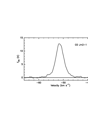
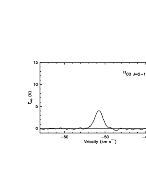
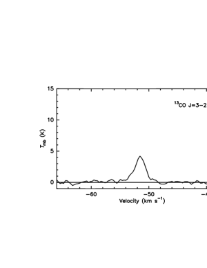
Figure 1: Spectra at the central position of the region (0, 0) of the mapping observations.

Table 1: Observational Parameters of the IRAS 22506+5944 Source

Name	$T_{\rm mb}$	FWHM	FW	$V_{\rm LSR}$
	${\rm(K)}$	${\rm(km\ s^{-1})}$	${\rm(km\ s^{-1})}$	${\rm(km\ s^{-1})}$
CO $J=2-1$	12.8$\pm$0.1	3.98$\pm$0.03	11.11	51.43$\pm$0.01
CO $J=3-2$	11.9$\pm$0.1	4.15$\pm$0.06	13.63	51.59$\pm$0.02
13CO $J=2-1$	4.1$\pm$0.1	2.37$\pm$0.04	6.69	51.52$\pm$0.02
13CO $J=3-2$	4.0$\pm$0.3	2.32$\pm$0.08	7.22	51.54$\pm$0.01

3.2 Dense Molecular Core

In Figure 2, all the structures of the molecular cloud core are presented and IRAS 22506+5944 has an isolated core. The cores in the $J=2-1$ transition lines have a similar morphology to those of the $J=3-2$ transition lines. Based on the results observed by other authors, there is a near-infrared source S4 which was detected by Wang (1997) as well as three H₂O masers in this region. The IRAS sources and the H₂O masers are located closer to the core peak position traced by the transition $J=2-1$, but a little deviation from that is also traced by the transition $J=3-2$. The IRAS sources are associated with the H₂O masers. This indicates that they are still undergoing activity in an early evolution stage (Felli et al. 1997). The H₂O masers occur in relatively warm environments. Using the IRAS point-source catalog, infrared luminosity (Casoli et al. 1986) and dust temperature (Henning et al. 1990) are given by, respectively:

$$\mathit{L}_{\rm IR}=(20.653\times F_{12}+7.358\times F_{25}+4.578\times F_{60}+1.762\times F_{100})\times D^{2}\times 0.30,$$ (1)

$$\mathit{T}_{D}=\frac{96}{(3+\beta)\ln(100/60)-\ln(F_{60}/F_{100})},$$ (2)

where $D$ is the distance from the sun in kpc; $F_{12}$, $F_{25}$, $F_{60}$, and $F_{100}$ are the infrared fluxes at four IRAS bands ($12\,\mu$m, 25 $\mu$m, 60 $\mu$m and 100 $\mu$m), respectively. The emissivity index of the dust particles ($\beta$) is assumed to be 2. The calculated results are presented in Table 2.

The core parameters are calculated following the procedure of Lee et al. (1990). Assuming LTE, we write the column density as

$$\mathit{N}=2.4\times 10^{14}\frac{\exp[hBJ(J+1)/kT_{\rm ex}]}{J+1}\times\frac{(T_{\rm ex}+hB/3\,{\rm K})\times\tau\times\Delta V}{1-\exp(-h\nu/kT_{\rm ex})}{\rm cm}^{-2},$$ (3)

where $B$ is the rotational constant of the molecule, $J$ is the rotational quantum number and $\nu$ is the frequency of the spectral line. $\Delta V$ is a half full-width of speed, $T_{\rm ex}$ is the excitation temperature and $\tau$ is the optical depth. Here we assume $N$(H₂)/$N$(CO)=$10^{4}$ (Dickman 1978).

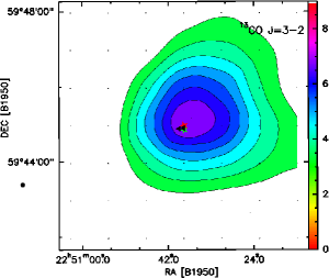
Figure 2: Integrated intensity maps of the core emission. In each map, the integrated range is from –53.26 to –49.68 ${\rm km\ s^{-1}}$. The contour levels are 30%, 40%,…, 90% of the peak value. The red star represents the IRAS 22506+5944 source position, the green star represents the near-infrared source S4, and the filled triangles indicate the positions of the three H₂O masers. The dot symbols mark the mapping points.

Table 2: IRAS Fluxes and Derived Parameters

Source	Distance	$F_{12}$	$F_{25}$	$F_{60}$	$F_{100}$	$\lg(F_{25}/F_{12})$	$\lg(F_{60}/F_{12})$	$T_{D}$	$L_{\rm IR}$
	(kpc)	($J_{\nu}$)	($J_{\nu}$)	($J_{\nu}$)	($J_{\nu}$)			(K)	($\times 10^{4}L_{\odot}$)
IRAS 22506+5944	5.1	6.37	34.74	187.50	295.10	0.74	1.47	31.90	1.38

The CO emission is always considered optically thick while the ¹³CO emission is usually optically thin. Therefore, the excitation temperature $T_{\rm ex}$(CO) is given by (Garden et al. 1991):

$$\mathit{T}_{\rm ex}({\rm CO})=\frac{hv}{k}\left({\ln\left\{1+\frac{hv}{k}{\left[\frac{T_{\rm mb}}{f}+\frac{hv}{k}\left(\exp\Big{(}\frac{hv}{kT_{\rm bg}}\Big{)}-1\right)\right]^{-1}}\right\}}\right)^{-1},$$ (4)

where $T_{\rm bg}$=2.732 K is the temperature of the cosmic background radiation, and $f$ is the beam filling factor. In addition, $\tau(^{13}$CO) is given by (Garden et al.1991):

$$\ \tau(^{13}{\rm CO})=-\ln{\left\{1-\frac{kT_{\rm mb}}{hv}\left[\frac{1}{\exp(hv/kT_{\rm ex})-1}-\frac{1}{\exp(hv/kT_{\rm bg})-1}\right]^{-1}\right\}}.$$ (5)

We also use another method to calculate $\tau(^{13}$CO):

$$\frac{T_{\rm mb}({\rm CO})}{T_{\rm mb}(^{13}{\rm CO})}\approx\frac{1-\exp[-\tau({\rm CO})]}{1-\exp[-\tau(^{13}{\rm CO})]}.$$ (6)

We assume the solar abundance ratio [CO]/[¹³CO]=$\tau($CO)/$\tau(^{13}$CO)=89 (Lang 1980). The calculated results are listed in Table 3. From the table, we can see that the optical depths calculated by the above two methods are almost equal. Thus, we suggest that the abundance ratio [CO]/[¹³CO] in this region is nearly the same as that in our solar system. Using the column density, the masses of outflow gas are obtained by:

$$\mathit{M}=\mu N_{\rm H_{2}}S/(2.0\times 10^{33}),$$ (7)

where the mean atomic weight of the gas $\mu$ is 1.36, and $S$ is the size of the core region. The physical parameters of the core are summarized in Table 4.

Table 3: Calculated Results of the Optical Depth

Name	$\tau_{1}$	$\tau_{2}$
CO $J=2-1$	33.55	34.00
CO $J=3-2$	52.33	53.59
13CO $J=2-1$	0.38	0.38
13CO $J=3-2$	0.59	0.60

The optical depth ($\tau_{1}$) is derived based on the first method. ($\tau_{2}$) is derived based on the second method.

Table 4: Physical Parameters of the Core

Name	$T_{\rm ex}$	$\tau$	$N$(CO $J=2-1$)	$N$(H2)	$M$
	(K)		($\times 10^{17}$cm-2)	($\times 10^{21}$cm-2)	($\times 10^{3}\,M_{\odot}$)
IRAS 22506+5944	20.5	33.55	7.07	7.07	2.03

3.3 The Bipolar Outflows

From Figure 3, bipolar outflows are clearly revealed in the IRAS 22506+5944 region. The red wing and blue wing lobes mostly overlap, which may be attributed to the axis of outflows being nearly parallel with the line of sight direction. The position-velocity (PV) diagrams in Figure 4, with a cut along the north-south direction, also clearly show high-velocity outflows. The outflows of the CO $J=3-2$ are much clearer than those of the CO $J=2-1$. Two IRAS sources are located close to the center of the outflows, so they may be the outflows driving the source, but we cannot distinguish which source is the driving source.

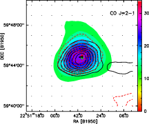
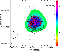
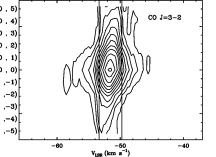
Figure 3: Left panel: outflow contours of the CO $J=2-1$ are superimposed on the integrated intensity map of the core; the integrated range is from –57.07 to –53.26 ${\rm km\ s^{-1}}$ for the blue wing (black solid line) and from –49.68 to –45.96 ${\rm km\ s^{-1}}$ for the red wing (red dashed line). Right panel: outflow contours of the CO $J=3-2$ are superimposed on the integrated intensity map of the core; the integrated range is from –58.96 to –53.26 ${\rm km\ s^{-1}}$ for the blue wing (black solid line) and from –49.68 to –45.33 ${\rm km\ s^{-1}}$ for the red wing (red dashed line). The contour levels for core and outflows are 30%, 40%, …, 90% of the peak values.

Figure 4: Left panel: P-V diagram constructed from the CO $J=2-1$ transition. Contour levels are 1, 2, 3, 4.5, 6, 6.5, 7.5, 9, 10.5, 12, 14,…, 25 K. Right panel: P-V diagram for CO $J=3-2$. Contour levels are the same as in the left panel. The left and right vertical lines indicate the beginning of the blue and red wings, respectively.

Under the LTE assumption, the averaged column density of the outflows can be obtained by (Scoville et al. 1986):

$$\mathit{N}=2.4\times 10^{14}\frac{\exp[hBJ(J+1)/kT_{\rm ex}]}{J+1}\times\frac{(T_{\rm ex}+hB/3\,{\rm K})}{\exp(-hv/kT_{\rm ex})}\int T_{\rm mb}\times\frac{\tau dv}{[1-\exp(-\tau)]}{\rm cm}^{-2}.$$ (8)

We consider that the excitation temperature is uniform in the observed region. The excitation temperature ($T_{\rm ex}$) is 20.5 K from the calculated results of the cores. The $\tau$ can be determined by Equation (6). The integral is carried out in the blue and red wing regions and the integrated ranges are determined from the PV diagram.

In addition, we can derive the outflows’ mass ($M$) from Equation (7). The momentum $P$ and energy $E$ are calculated by $P=MV$ and $E=MV^{2}$, where $V$ is the mean velocity of the gas relative to the cloud’s systemic velocity. A dynamic time scale can be determined by $t_{\rm d}=R/V$, where $R$ is the mean size of the outflows. The driving force is determined by $F=P/t_{\rm d}$. The mechanical luminosity and the mass loss rate of the outflows are calculated using $L_{\rm mech}=E/t_{\rm d}$ and $\dot{M}=P/(t_{\rm d}v_{\rm w})$, where the final wind velocity is taken to be $v_{\rm w}=500\,{\rm km\ s^{-1}}$ (Marti et al. 1986). The calculated results are listed in Table 5.

Table 5: Physical Parameters of the Outflows

Name	Wing	$N$(H2)	$M$	$t_{\rm d}$	$\dot{M}$	$F$	$P$	$E$	$L_{\rm Mech}$
IRAS		($\times 10^{20}$ cm-2)	($M_{\odot}$)	($\times 10^{5}$ yr)	($M_{\odot}$ yr-1)	($M_{\odot}$ km s-1 yr-1)	($M_{\odot}$ km s-1)	($\times 10^{46}$ erg)	($L_{\odot}$)
22506+5944	Blue	1.35	18.7	4.14	$8.0\times 10^{-7}$	$4.0\times 10^{-4}$	164.6	1.08	0.22
	Red	1.35	18.6	4.38	$8.2\times 10^{-7}$	$4.1\times 10^{-4}$	179.6	1.30	0.24

4 Discussion

From Figure 1 and Table 1, the full width of the CO $J=3-2$ line is larger than that of the CO $J=2-1$ line and the line wings in CO $J=2-1$ are broader than those in CO $J=1-0$ (Wu et al. 2005). These results suggest that the outflows may be caused by stellar wind sweeping up the surrounding materials in different intensity layers and the outflows traced by the higher $J$ level CO lines arise from the warm layer closer to the central exciting star.

Although the color indexes of the source satisfy the criteria of Wood $\&$ Churchwell (1989), they are not detected in the centimeter or millimeter continuum emission (Wu et al. 2005). Whether or not it is a UC HII region still needs to be determined by further higher sensitivity continuum observations. So far, the majority of authors have used constant values of $\tau$ and $T_{\rm ex}$ to estimate total mass. Because our observations were simultaneously made in CO and ¹³CO, we can obtain relatively accurate values of $\tau$ and $T_{\rm ex}$, as well as the total mass. From Table 4, the total mass of the core is 2.03$\times 10^{3}\,M_{\odot}$; the value indicates that IRAS 22506+5944 is a high-mass star formation region. Wang (1997) found clusters of stellar objects and an infrared jet in this region. Thus, we conclude that IRAS 22506+5944 is associated with molecular cloud complexes. The IRAS 22506+5944 source appears to be a deeply embedded protostar.

In addition, the contour maps and PV diagram of the IRAS 22506+5944 source clearly show bipolar outflows in this region. The total mass of the outflows is 37.3 $M_{\odot}$, and the total amount of momenta is 344.2 $M_{\odot}$ km s^-1. Both parameters are much larger than the typical values in low-mass outflows. The larger outflow’s mass suggests that the outflows’ mass is not likely to originate from the stellar surface, but could be caused by the entrainment of ambient gas (Shepherd $\&$ Churchwell 1996). The IRAS 22506+5944 source is considered as the outflow driving source by Su et al. (2004), while Wu et al. (2005) consider S4 to be the outflow driving source. Two IRAS sources are located at the geometric position of the driving source of the outflow, and we also cannot identify which one is the driving source. We need to apply for observations with a much higher angular resolution telescope to confirm it. $L_{\rm IR}/L_{\rm Mech}\gg 1$, and $L_{\rm IR}/CF<1$, where $L_{\rm Mech}$ is the total mechanical luminosity, suggesting that despite the strong radiation from the central source, the radiation pressure still cannot supply enough force to drive such massive outflows (Wu et al. 1998).

5 Conclusions

We observed the CO $J=2-1$, CO $J=3-2$, ¹³CO $J=2-1$ and ¹³CO $J=3-2$ lines in the direction of IRAS 22506+5944. IRAS 22506+5944 has an isolated core. The infrared data indicate that the IRAS 22506 +5944 source appears to be a deeply embedded protostar. Bipolar outflows are further identified in this region. IRAS 22506+5944 or NIR source S4 may be the outflow driving source. The two IRAS sources are associated with H₂O masers. The H₂O masers occur in relatively warm environments. The parameters of the core and the outflows are derived; the derived values suggest that IRAS 22506 +5944 is a high-mass star formation region and the total mass of the outflows is larger than that in low-mass star formation regions. Compared with the extension of line wings in CO $J=2-1$, CO $J=3-2$ line wings extend further in velocity, suggesting that the outflows traced by the higher $J$ level ¹²CO lines arise from the warm layer closer to the central exciting star.

- (1) Casoli, F., Combes, F., Dupraz, C., Gerin, M., & Boulanger, F. 1986, A&A, 169, 281
- (2) Dickman, R. L. 1978, ApJ, 37, 407
- (3) Elitzur, M., Hollenbach, D. J., & McKee, C. F. 1989, ApJ, 346, 983
- (4) Felli, M., Testi, L., Valdettaro, R., & Wang, J. J. 1997, A&A, 320, 594
- (5) Garden, P. R., Hayashi, M., Hasegawa, T., Gatley, I., & Kaifu, N. 1991, ApJ, 374, 540
- (6) Henning, Th., Pfau, W., & Altenhoff, W. J. 1990, A&A, 227, 542
- (7) Jenness, T., Scott, P. F., & Padman, R. 1995, MNRAS, 276, 1024
- (8) Lada, E. A., Strom, K. M., & Myers, P. C. 1993, Protostars and Planets III, eds. E. H. Levy, & J. I. Lunine (Tucson: Univ. Arizonna Press), 245
- (9) Lang, K. R. 1980 Astrophysical Formulae (Berlin: Springer-Verlag)
- (10) Lee, Y., Snell, R. L., & Dickman, R. L. 1990 ApJ, 355, 536
- (11) Marti, J., Rodriguez, L. F., & Reipurth, B. 1998 ApJ, 502, 377
- (12) Molinari, S., Brand, J., Cesaroni, R., & Palla, F. 1998 A&A, 308, 573
- (13) Scoville, N. Z., Sargent, A. I., Sanders, D. B., et al. 1986, ApJ, 303, 416
- (14) Shepherd, D. S., & Churchwell, E. 1989, ApJ, 340, 265
- (15) Shepherd, D. S., & Churchwell, E. 1996, ApJ, 472, 225
- (16) Shu, F. H., Adams, F. C., & Lizano, S. 1987, ARA&A, 25, 23
- (17) Su, Y.-N., Zhang, Q., & Lim, J. 2004, ApJ, 604, 258
- (18) Wang, J. J. 1997, Ph.D.Thesis, Beijing Astron. Obs.
- (19) Wood, D. O. S., & Churchwell, E. 1989, ApJ, 340, 265
- (20) Wu, Y., et al. 1998, A&AS, 18, 243
- (21) Wu, Y., Zhang, Q., Chen, H., Yang, C., Wei, Y., et al. 2005, AJ, 129, 330
- (22) Zhang, Q., Hunter, T. R., Brand, J., et al. 2001, ApJ, 552, 167