We present simulations of atmospheres of Earth-like aquaplanets that are tidally locked to their star, that is, planets whose orbital period is equal to the rotation period about their spin axis, so that one side always faces the star and the other side is always dark. As extreme cases illustrating the effects of slow and rapid rotation, we consider planets with rotation periods equal to one current Earth year and one current Earth day. The dynamics responsible for the surface climate (e.g., winds, temperature, precipitation) and the general circulation of the atmosphere are discussed in light of existing theories of atmospheric circulations. For example, as expected from the increasing importance of Coriolis accelerations relative to inertial accelerations as the rotation rate increases, the winds are approximately isotropic and divergent at leading order in the slowly rotating atmosphere but are predominantly zonal and rotational in the rapidly rotating atmosphere. Free-atmospheric horizontal temperature variations in the slowly rotating atmosphere are generally weaker than in the rapidly rotating atmosphere. Interestingly, the surface temperature on the night side of the planets does not fall below $\mathop{\sim}\!240\,\mathrm{K}$ in either the rapidly or slowly rotating atmosphere; that is, heat transport from the day side to the night side of the planets efficiently reduces temperature contrasts in either case. Rotational waves and eddies shape the distribution of winds, temperature, and precipitation in the rapidly rotating atmosphere; in the slowly rotating atmosphere, these distributions are controlled by simpler divergent circulations. The results are of interest in the study of tidally locked terrestrial exoplanets and as illustrations of how planetary rotation and the insolation distribution shape climate.

1 Introduction

Planets generally evolve toward a state in which they become tidally locked to their star. Torques the star exerts on tidal bulges on a planet lead to an exchange between the spin angular momentum of the planetary rotation and orbital angular momentum of the planet’s revolution around the star, such that the rotation period around the spin axis gradually approaches the orbital period of the planet (Hubbard 1984). (The spin angular momentum of the star may also participate in this angular momentum exchange.) This process reaches its tidally locked end state when the rotation period is equal to the orbital period, so that one side of the planet always faces the star and the other side is always dark. The time it takes to reach this end state may exceed the lifetime of the planetary system, so it may never be reached (this is almost certainly the case for the Sun-Earth system). But planets that are close to their star can reach a tidally locked state more quickly. Such close planets in other solar systems are easier to detect than planets farther away from their star, and exoplanets that are believed to be tidally locked have indeed been detected in recent years (e.g., Charbonneau et al. 2000). Here we investigate the atmospheric dynamics of Earth-like tidally locked aquaplanets through simulations with a three-dimensional general circulation model (GCM). Our purpose is pedagogic: we contrast rapidly and slowly rotating tidally locked Earth-like planets with each other and with Earth itself to illustrate the extent to which atmospheric dynamics depend on the insolation distribution and planetary rotation rate.

There are two areas of existing research on the atmospheric dynamics of tidally locked planets. First, there are several studies motivated by “hot Jupiters”—large, close-in planets that have been observed transiting a star (see Showman et al. (2009) for a review). Second, there are studies of Earth-like exoplanets closely orbiting a relatively cool star—planets that have not yet been but may be detected soon, for example, by NASA’s recently launched Kepler space telescope or by ground-based telescopes (as demonstrated by the observations of Charbonneau et al. 2009). Joshi et al. (1997) investigated the large-scale circulation of such Earth-like planets and explored how their climate depends on the mass of the atmosphere. And Joshi (2003) documented their hydrological cycle using an Earth climate model.

The studies by Joshi et al. provide a description of Earth-like tidally locked atmospheric circulations and how they depend on some parameters, such as the atmospheric mass. But some questions remain, among them: (i) How does the planet’s rotation rate affect the circulation and climate? (ii) What controls the precipitation distribution (location of convergence zones)? (iii) What mechanisms generate large-scale features of the circulation, such as jets? (iv) What determines the atmospheric stratification?

We address these questions by simulating tidally locked Earth-like aquaplanets with rotation periods equal to one current Earth year and one current Earth day. These are merely two illustrative cases: The slowly rotating case corresponds roughly to the tidally locked end state Earth would reach if the sun were not changing, that is, if the solar constant $S_{0}=1367\ \mathrm{Wm}^{-2}$ remained fixed. The rapidly rotating case corresponds to a terrestrial planet sufficiently close to a cool host star, so that the orbital period is one Earth day but the average insolation reaching the planet still is $S_{0}=1367\ \mathrm{Wm}^{-2}$, as presently on Earth.

2 General circulation model

We use an idealized atmosphere GCM with an active hydrological cycle and an aquaplanet (slab ocean) lower boundary condition. The slab ocean has no explicit horizontal transports but is implicitly assumed to transport water from regions of net precipitation to regions of net evaporation, so that the local water supply is unlimited. The GCM is a modified version of the model described in O’Gorman and Schneider (2008), which is similar to the model described in Frierson et al. (2006). Briefly, the GCM is a three-dimensional primitive-equation model of an ideal-gas atmosphere. It uses the spectral transform method in the horizontal, with resolution T85, and finite differences in $\sigma=p/p_{s}$ coordinates (pressure $p$ and surface pressure $p_{s}$) in the vertical, with $30$ unequally spaced levels. Subgrid-scale dissipation is represented by an exponential cutoff filter (Smith et al. 2002), which acts on spherical wavenumbers greater than 40, with a damping timescale of $1\,\mathrm{h}$ on the smallest resolved scale. Most features of the simulated flows are similar at T42 resolution or with different subgrid-scale filters; exceptions are noted below.

The GCM has a surface with uniform albedo ($0.38$) and uniform roughness lengths for momentum fluxes ($5\times 10^{-3}\,\mathrm{m}$) and for latent and sensible heat fluxes ($10^{-5}\,\mathrm{m}$). It has a gray radiation scheme, and a quasi-equilibrium moist convection scheme that relaxes convectively unstable atmospheric columns to a moist pseudo-adiabat with constant relative humidity $70\%$ (Frierson 2007). Only the vapor-liquid phase transition is taken into account, and the latent heat of vaporization is taken to be constant. No liquid water is retained in the atmosphere, so any precipitation that forms immediately falls to the surface. Radiative effects of clouds are not taken into account, except insofar as the surface albedo and radiative parameters are chosen to mimic some of the global-mean effects of clouds on Earth’s radiative budgets.

Other model details can be found in O’Gorman and Schneider (2008). However, the radiation scheme differs from that in O’Gorman and Schneider (2008) and is described in what follows.

a Tidally locked insolation

The top-of-atmosphere insolation is held fixed at the instantaneous value for a spherical planet (e.g., Hartmann 1994),

$$S_{\mathrm{TOA}}=S_{0}\times\mathrm{max}\bigl{(}0,\cos(\phi)\cos(\lambda-\lambda_{0})\bigr{)},$$ (2.1)

where $\phi$ is latitude and $\lambda$ is longitude, with subsolar longitude $\lambda_{0}=270^{\circ}$ and solar constant $S_{0}=1367\ \mathrm{Wm}^{-2}$. There is no diurnal cycle of insolation. That is, we assume zero eccentricity of the orbit and zero obliquity of the spin axis.

b Longwave optical depth

O’Gorman and Schneider (2008) used a gray radiation scheme with a longwave optical depth that was uniform in longitude and a prescribed function of latitude, thereby ignoring any longwave water vapor feedback. This is not adequate for tidally locked simulations with strong radiative variations in longitude. Therefore, we use a longwave optical depth that varies with the local water vapor concentration (cf. Thuburn and Craig 2000), providing a crude representation of longwave water vapor feedback.

As in Frierson et al. (2006), the longwave optical depth $\tau$ has a term linear in pressure $p$, representing well-mixed absorbers like CO₂, and a term quartic in pressure, representing water vapor, an absorber with a scale height that is one quarter of the pressure scale height,

$$\tau=\tau_{0}\left(\frac{p}{p_{0}}\right)^{4}+\tau_{1}\left(\frac{p}{p_{0}}\right).$$ (2.2)

Here, $\tau_{1}=1.2$ and $p_{0}=10^{5}\,\mathrm{Pa}$ are constants. However, the optical thickness of water vapor is a function of the model’s instantaneous column water vapor concentration,

$$\tau_{0}=\frac{1}{p_{1}}\int_{0}^{p_{s}}q\,dp,$$ (2.3)

with specific humidity $q$ and an empirical constant $p_{1}=980\,\mathrm{Pa}$ to keep $\tau_{0}$ order one for conditions typical of Earth’s tropics.

The details of the radiation scheme such as the constants chosen affect quantitative aspects of the simulations (e.g., the precise surface temperatures obtained), but not the large-scale dynamics on which we focus. The simulated surface climate is similar to those presented in Joshi (2003), who used a more complete representation of radiation including radiative effects of clouds. This gives us confidence that the qualitative results presented here do not depend on the details of the radiation scheme.

c Simulations

We conducted a rapidly rotating simulation with planetary rotation rate equal to that of present-day Earth, $\Omega=\Omega_{E}=7.292\times 10^{-5}\mathrm{s}^{-1}$, and a slowly rotating simulation with planetary rotation rate approximately equal to one present-day Earth year, $\Omega=\Omega_{E}/365$.

The results we present are averages over the last 500 days of 4000-day simulations (with 1 day = $86400\,\mathrm{s}$, irrespective of the planetary rotation rate). During the first 3000 days of the simulation, we adjusted the subgrid-scale dissipation parameters to the values stated above to ensure there was no energy build-up at the smallest resolved scales.

3 Slowly rotating simulation

The Rossby number $\mathrm{Ro}=U/(fL)$, with horizontal velocity scale $U$, Coriolis parameter $f$, and length scale $L$, is a measure of the importance of inertial accelerations ($\mathop{\sim}\!U^{2}/L$) relative to Coriolis accelerations ($\mathop{\sim}\!fU$) in the horizontal momentum equations. In rapidly rotating atmospheres, including Earth’s, the Rossby number in the extratropics is small, and the dominant balance is geostrophic, that is, between pressure gradient forces and Coriolis forces. In slowly rotating atmospheres, the Rossby number may not be small. If $\mathrm{Ro}=O(1)$, inertial and Coriolis accelerations both are important, as in the deep tropics of Earth’s atmosphere. If $\mathrm{Ro}\gg 1$, Coriolis accelerations and effects of planetary rotation become unimportant. In that case, there is no distinguished direction in the horizontal momentum equations, so the horizontal flow is expected to be isotropic, that is, the zonal velocity scale $U$ and meridional velocity scale $V$ are of the same order. This is the dynamical regime of our slowly rotating simulation.

In this dynamical regime, the magnitude of horizontal temperature variations can be estimated through scale analysis of the horizontal momentum equations (Charney 1963). In the free atmosphere, where frictional forces can be neglected, inertial accelerations scale advectively, like $\mathop{\sim}\!U^{2}/L$, and are balanced by accelerations owing to pressure gradients, which scale like $\delta p/(\rho L)$, where $\delta p$ is the scale of horizontal pressure variations and $\rho$ is density. The density and vertical pressure variations are related by the hydrostatic relation, $p/H\sim\rho g$, where $H=RT/g$ is the pressure scale height (specific gas constant $R$ and temperature $T$). If one combines the scalings from the horizontal momentum and hydrostatic equations, horizontal variations in pressure, density, and (potential) temperature (using the ideal gas law) scale like

$$\frac{\delta p}{p}\sim\frac{\delta\rho}{\rho}\sim\frac{\delta\theta}{\theta}\sim\frac{U^{2}}{gH}\equiv\mathrm{Fr},$$ (3.1)

where $\mathrm{Fr}=U^{2}/(gH)$ is the Froude number. For a terrestrial planet with $H\approx 7\,\mathrm{km}$ and $g=9.8\,\mathrm{m\,s^{-2}}$, the Froude number is $\mathrm{Fr}\lesssim 10^{-2}$ for velocities $U\lesssim 25\,\mathrm{m\,s^{-1}}$. So free-atmospheric horizontal temperature and pressure variations are expected to be small insofar as velocities are not too strong (e.g., if their magnitude is limited by shear instabilities). This is the case in the tropics of Earth’s atmosphere, and these expectations are also borne out in the slowly rotating simulation.

a Surface temperature

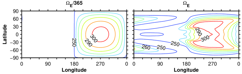
Figure 1: Surface temperature (K) in simulations with $\Omega_{E}/365$ (left) and $\Omega_{E}$ (right). The contour interval is $10\,\mathrm{K}$.

In the slowly rotating simulation, the surface temperature mimics the insolation distribution on the day side of the planet, decreasing monotonically and isotropically away from the subsolar point; the night side of the planet has a nearly uniform surface temperature (Fig. 1). Though the surface temperature resembles the insolation distribution, the influence of atmospheric dynamics is clearly evident in that the night side of the planet is considerably warmer than the radiative-convective equilibrium temperature of $0\,\mathrm{K}$.

b Hydrological cycle

Figure 2: Evaporation (top row, mm/day), precipitation (middle row, mm/day), and evaporation minus precipitation (bottom row, mm/day) in simulations with $\Omega_{E}/365$ (left) and $\Omega_{E}$ (right). Contours are shown at $0.1\times 5^{0,1,2,3,4}\,\mathrm{mm\,day^{-1}}$ in the top two rows and $-12.5,-1.0,0,1.0,12.5\,\mathrm{mm\,day^{-1}}$ in the bottom row.

Surface evaporation rates likewise mimic the insolation distribution (Fig. 2), as would be expected from a surface energy budget in which the dominant balance is between heating by shortwave radiation and cooling by evaporation. This is the dominant balance over oceans on Earth (e.g., Trenberth et al. 2009), and in general on sufficiently warm Earth-like aquaplanets (Pierrehumbert 2002; O’Gorman and Schneider 2008). The dominance of evaporation in the surface energy budget in sufficiently warm climates can be understood by considering how the Bowen ratio, the ratio of sensible to latent surface fluxes, depends on temperature. For surface fluxes given by bulk aerodynamic formulas, the Bowen ratio, $B$, depends on the surface temperature, $T_{s}$, the near-surface air temperature, $T_{a}$, and the near-surface relative humidity, $\mathcal{H}$,

$$B\sim\frac{c_{p}(T_{s}-T_{a})}{L\bigl{(}q^{*}(T_{s})-\mathcal{H}q^{*}(T_{a})\bigr{)}},$$ (3.2)

where $q^{*}$ is the saturation specific humidity, $c_{p}$ is the specific heat of air at constant pressure, and $L$ is the latent heat of vaporization. Fig. 3 shows the Bowen ratio as a function of surface temperature, assuming a fixed surface–air temperature difference and fixed relative humidity. We have fixed these to values that are representative of the GCM simulations for simplicity, but the surface–air temperature difference and relative humidity are not fixed in the GCM. For surface temperatures greater than $\mathop{\sim}\!290\,\mathrm{K}$, latent heat fluxes are a factor of $\gtrsim 4$ larger than sensible heat fluxes, as at Earth’s surface (Trenberth et al. 2009). Similar arguments apply for net longwave radiative fluxes at the surface, which become small as the longwave optical thickness of the atmosphere and with it surface temperatures increase; see Pierrehumbert (2009) for a more complete discussion of the surface energy budget.

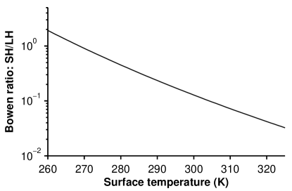
Figure 3: Bowen ratio vs surface temperature assuming a 3-K surface–air temperature difference, 70% relative humidity, and surface and surface air pressure of $10^{5}$ Pa, using the same simplified saturation vapor pressure formula as in the GCM.

The precipitation rates also mimic the insolation distribution (Fig. 2). There is a convergence zone with large precipitation rates ($\geq 40\,\mathrm{mm/day}$) around the subsolar point. Precipitation rates exceed evaporation rates within $\mathop{\sim}\!15^{\circ}$ of the subsolar point. Outside that region on the day side, evaporation rates exceed precipitation rates (Fig. 2), which would lead to the generation of deserts there if the surface water supply were limited. The atmospheric circulation that gives rise to the moisture transport toward the subsolar point is discussed next.

c General circulation of the atmosphere

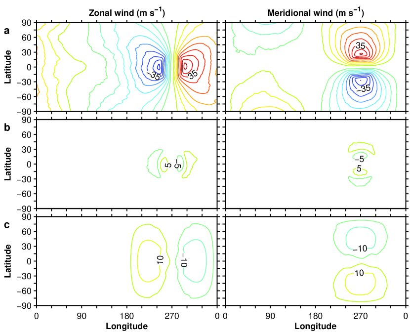
Figure 4: Zonal wind (left) and meridional wind (right) in $\Omega_{E}/365$ simulation on the $\sigma=0.28$ (a), $0.54$ (b), and $1.0$ (c) surfaces. The contour interval is $5\,\mathrm{m\,s^{-1}}$.

The winds are approximately isotropic and divergent at leading order. They form a thermally direct overturning circulation, with lower-level convergence near the subsolar point, upper-level divergence above it, and weaker flow in between (Fig. 4). As in the simulations of Joshi et al. (1997), the meridional surface flow crosses the poles. Moist convection in the vicinity of the subsolar point results in strong mean ascent in the mid-troposphere there; elsewhere there is weak subsidence associated with radiative cooling (Fig. 5). Consistent with the predominance of divergent and approximately isotropic flow, the Rossby number is large even in the extratropics ($\mathrm{Ro}\gtrsim 10$).

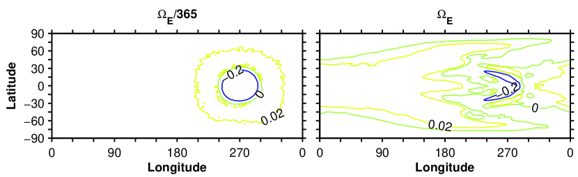
Figure 5: Pressure velocity ($\omega=Dp/Dt$) on the $\sigma=0.54$ surface in simulations with $\Omega_{E}/365$ (left) and $\Omega_{E}$ (right). Contours are shown at $-0.2$, $0$, and $0.02\,\mathrm{Pa\,s^{-1}}$.

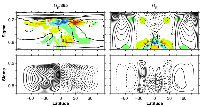
Figure 6: Circulation in simulations with $\Omega_{E}/365$ (left panels) and $\Omega_{E}$ (right panels). Top row: zonal mean zonal wind (lines, contour interval $1\,\mathrm{m\,s^{-1}}$ for $\Omega_{E}$ and $5\,\mathrm{m\,s^{-1}}$ for $\Omega_{E}/365$) and divergence of the horizontal component of eddy (transient and stationary) angular momentum fluxes (colors, contour interval $1.0\times 10^{-6}\,\mathrm{m\,s^{-2}}$ for $\Omega_{E}/365$ and $1.5\times 10^{-5}\,\mathrm{m\,s^{-2}}$ for $\Omega_{E}$). Bottom row: Eulerian-mean mass flux streamfunction (contour interval $25\times 10^{9}\,\mathrm{kg\,s^{-1}}$ for $\Omega_{E}/365$ and $10\times 10^{9}\,\mathrm{kg\,s^{-1}}$ for $\Omega_{E}$).

The zonal mean zonal wind and streamfunction are shown in Fig. 6. The zonal mean zonal wind is a weak residual of the opposing contributions from different longitudes (Fig. 4). In the upper troposphere near the equator, there are weak westerly (superrotating) zonal winds, as well as the eddy angular momentum flux convergence that, according to Hide’s theorem, is necessary to sustain them (e.g., Hide 1969; Schneider 1977; Held and Hou 1980; Schneider 2006).

The Eulerian mean mass streamfunction consists of a Hadley cell in each hemisphere, which is a factor $\mathop{\sim}\!3$ stronger than Earth’s and extends essentially to the pole. These Hadley cells are thermodynamically direct circulations: the poleward flow to higher latitudes has larger moist static energy ($h=c_{p}T+gz+Lq$) than the near-surface return flow. The classic theory of Hadley cells with nearly inviscid, angular momentum-conserving upper branches predicts that the Hadley cell extent increases as the rotation rate decreases (Schneider 1977; Held and Hou 1980). However, the results of this theory do not strictly apply here because several assumptions on which it is based are violated. For example, the surface wind is not weak relative to the upper-tropospheric winds (Fig. 4), and the zonal wind is not in balance with meridional geopotential (or temperature) gradients (i.e., the meridional wind is not negligible in the meridional momentum equation). Nonetheless, it is to be expected that Hadley cells in slowly rotating atmospheres span hemispheres (Williams 1988).

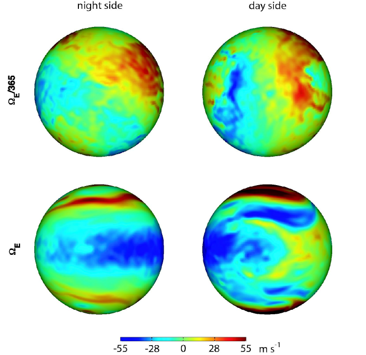
Figure 7: Instantaneous zonal wind on $\sigma=0.28$ surface in the statistically steady state (on day 3900) of the two simulations. Animations are available at _anim and _anim .

The instantaneous, upper-tropospheric zonal wind is shown in Fig. 7, and a corresponding animation is available at _anim. Athough the flow statistics in the simulations are hemispherically symmetric (because the forcing and boundary conditions are), the instantaneous wind exhibits north-south asymmetries on large scales and ubiquitous variability on smaller scales. The large-scale variability has long timescales ($\mathop{\sim}\!80$ days), and the zonal-mean zonal wind is sensitive to the length of the time averaging: for timescales as long as the 500 days over which we averaged, the averages still exhibit hemispheric asymmetries (Fig. 6).

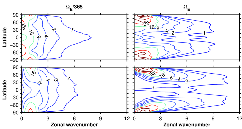
Figure 8: Spectrum of the mass-weighted, vertically averaged transient velocity variance for zonal (top row) and meridional (bottom row) wind components in the simulations with $\Omega_{E}/365$ (left) and $\Omega_{E}$ (right). Contours are shown at $2^{0},2^{1},...,2^{5}\,\mathrm{m^{2}\,s^{-2}}$.

The vertically integrated eddy kinetic energy is $8.4\times 10^{5}\ \mathrm{J\ m^{-2}}$ in the global mean. The instantaneous velocity fields exhibit substantial variability on relatively small scales (e.g., Fig. 7), and the kinetic energy spectrum decays only weakly from spherical wavenumber $\mathop{\sim}\!20$ toward the roll-off near the grid scale owing to the subgrid-scale filter. However, the peak in velocity variance is at the largest scales (Fig. 8)—as suggested by the hemispherically asymmetric large-scale variability seen in Fig. 7 and in the animation.

d Atmospheric stratification and energy transports

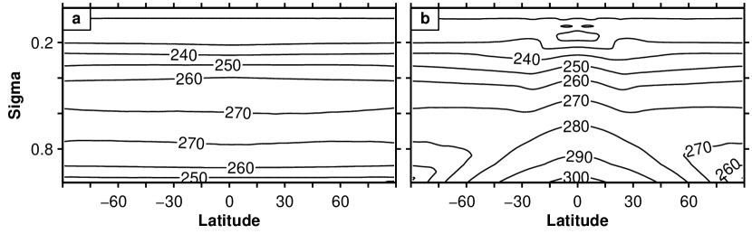
Figure 9: Temperature section of antisolar longitudes (a) and subsolar longitudes (b) of $\Omega_{E}/365$ simulation. Averages are taken over 10^∘ of longitude. The contour interval is $10\,\mathrm{K}$.

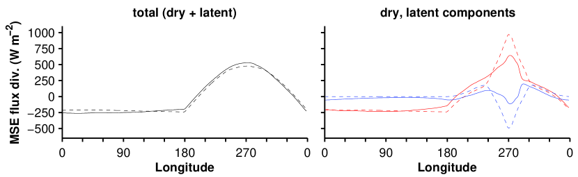
Figure 10: Left: Vertical and meridional integral of the divergence of the moist static energy flux, $uh$. Right: Dry static energy (red) and latent energy (blue) components of moist static enery flux divergence. Dashed lines for $\Omega_{E}/365$ simulation and solid lines for $\Omega_{E}$ simulation.

Consistent with the scaling arguments presented above, horizontal variations in temperature are small in the free troposphere (above the $\mathop{\sim}\!750$ hPa level, Fig. 9). This is reminiscent of Earth’s tropics, where temperature variations are small because Coriolis accelerations are weak compared with inertial accelerations (e.g., Charney 1963; Sobel et al. 2001). Here, Coriolis accelerations are weak at all latitudes, and free-tropospheric horizontal temperature variations are small everywhere.

The thermal stratification on the day side in the simulation is moist adiabatic in the free troposphere within $\mathop{\sim}\!30^{\circ}$ of the subsolar point. Farther away from the intense moist convection around the subsolar point, including on the night side of the planet, there are low-level temperature inversions (Fig. 9b), as in the simulations in Joshi et al. (1997). These regions have small optical thickness because of the low water vapor concentrations and therefore have strong radiative cooling to space from near the surface. The inversions arise because horizontal temperature gradients are constrained to be weak in the free troposphere, but near-surface air cools strongly radiatively, giving rise to inversions.

The vertical and meridional integral of the horizontal moist static energy flux divergence as a function of longitude is shown in Fig. 10 (dashed curves). Energy diverges on the day side of the planet and converges on the night side of the planet, reducing temperature contrasts. Near the subsolar point, there is substantial cancellation between the latent energy and dry static energy components of the moist static energy flux divergence as there is, for example, in Earth’s Hadley circulation. As can be inferred from the minimal water vapor flux divergence on the night side (Fig.  2), the moist static energy flux divergence is dominated by the dry static energy ($c_{p}T+gz$) component on the night side ($\gtrsim 99\%$ of the total).

4 Rapidly rotating simulation

In rapidly rotating atmospheres, the Rossby number in the extratropics is small, and geostrophic balance is the dominant balance in the horizontal momentum equations. In the zonal mean, zonal pressure gradients vanish, but meridional pressure gradients do not, so if the dominant momentum balance is geostrophic, winds are anisotropic $\overline{U}>\overline{V}$, where $\overline{(\cdot)}$ denotes a zonal mean. Variations in the planetary vorticity with latitude, $\beta$, are central to vorticity mixing arguments (e.g., Rhines 1994; Held 2000), which can account for the generation of atmospheric jets: When a Rossby wave packet stirs the atmosphere in a region bounded by a polar cap, high-vorticity fluid moves equatorward and low-vorticity fluid moves poleward. This reduces the vorticity in the polar cap. By Stokes’ Theorem, the reduced vorticity in the polar cap means the zonal wind at the latitude of the bounding cap decreases; if angular momentum is conserved, the zonal wind outside the polar cap increases. Irreversible vorticity mixing (wave-breaking or dissipation) is necessary to maintain the angular momentum fluxes in the time mean. Thus, the larger planetary vorticity gradients of the rapidly rotating planet allow jets to form provided there is a source of wave activity that leads to vorticity stirring.

We return to the analysis of Charney (1963) to estimate temperature variations in the free atmosphere. For rapidly rotating planets, geostrophic balance holds in the horizontal momentum equations: $\delta p/(\rho L)\sim fU$. Combining the scaling from the momentum equation with the hydrostatic relation, the pressure, density, and (potential) temperature variations scale like the ratio of the Froude number to the Rossby number,

$$\frac{\delta p}{p}\sim\frac{\delta\rho}{\rho}\sim\frac{\delta\theta}{\theta}\sim\frac{fUL}{gH}=\frac{\mathrm{Fr}}{\mathrm{Ro}}.$$ (4.1)

Where the Rossby number is small (in the extratropics), the temperature variations will be a factor of order inverse Rossby number ($\mathrm{Ro}^{-1}\sim 10$) larger than in the slowly rotating simulation if similar values for $U,g,$ and $H$ are assumed. Thus, we expect larger horizontal temperature and pressure variations away from the equator in the rapidly rotating simulation.

a Surface temperature

In the rapidly rotating simulation, the surface temperature on the day side of the planet is maximal off of the equator and does not bear a close resemblance to the insolation distribution; the night side of the planet has relatively warm regions in western high latitudes (Fig. 1). Compared to the slowly rotating simulation, the surface temperature is more substantially modified by the atmospheric circulation; however, the temperature contrasts between the day and night side are similar.

b Hydrological cycle

Surface evaporation rates mimic the insolation distribution (Fig. 2). This is one of the most similar fields between the slowly and rapidly rotating simulations, as expected from the gross similarity in surface temperature and the smallness of the Bowen ratio at these temperatures (Fig. 3). This might not be the case if the model included the radiative effects of clouds since the amount of shortwave radiation reaching the surface would be shaped by variations in cloud albedo which, in turn, depend on the atmospheric circulation.

Precipitation rates are large in a crescent-shaped region on the day side of the planet; the night side of the planet generally has small but nonzero precipitation rates (Fig. 2). The evaporation minus precipitation field has substantial structure: there are large amplitude changes from the convergence zones ($P>E$) to nearby areas of significant net drying ($E>P$). Comparing the slowly and rapidly rotating simulations shows that precipitation and $E-P$ on the night side of the planet are sensitive to the atmospheric circulation.

An interesting aspect of the climate is that the maximum precipitation (near $\mathop{\sim}\!15^{\circ}$ latitude) is not co-located with the off-equator maximum surface temperature (near $\mathop{\sim}\!40^{\circ}$ latitude). The simulation provides an example of precipitation and deep convection that are not locally thermodynamically controlled: the precipitation is not maximum where the surface temperature is maximum; the column static stability (e.g., Fig. 13), and therefore the convective available potential energy, are not markedly different between the maxima in precipitation and temperature. However, if the surface climate is examined latitude-by-latitude instead of examining its global maxima, the region of large precipitation is close to the maximum surface temperature (as well as surface temperature curvature) at a given latitude. The structure of the surface winds, discussed next, and the associated moisture convergence are key for determining where precipitation is large. Sobel (2007) provides a review of these two classes of theories for tropical precipitation (thermodynamic control vs. momentum control) and the somewhat inconclusive evidence of which class of theory better accounts for Earth observations.

The global precipitation is $\sim$10% larger in the rapidly rotating simulation than in the slowly rotating simulation. This suggests that radiative-convective equilibrium cannot completely describe the strength of the hydrological cycle.

c General circulation of the atmosphere

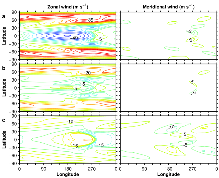
Figure 11: Zonal wind (left) and meridional wind (right) of $\Omega_{E}$ simulation on the $\sigma=0.28$ (a), $0.54$ (b), and $1.0$ (c) surfaces. The contour interval is $5\,\mathrm{m\,s^{-1}}$.

In the rapidly rotating simulation, the atmospheric circulation has several prominent features: there are westerly jets in high ($\mathop{\sim}\!65^{\circ}$) latitudes, the mid-tropospheric zonal wind exhibits superrotation, and the surface winds converge in a crescent-shaped region near the subsolar point (Fig. 11). The equatorial superrotation and westerly jets are clear in the zonal mean zonal wind (Fig. 6).

The existence of the high-latitude jets can be understood from the temperature field and eddy angular momentum flux convergence (Figs. 13 and  6). There are large meridional temperature gradients, which give rise to zonal wind shear by thermal wind balance and provide available potential energy for baroclinic eddies that transport angular momentum into the jets. In the vertical average, the eddy angular momentum transport into an atmospheric column is balanced by surface stress. Note that the region of higher temperatures on the night side of the planet coincides with the westerly jet’s surface maximum. The stronger winds at these latitudes lead to strong temperature advection. The equatorial superrotation is a consequence of angular momentum flux convergence (Fig. 6). Saravanan (1993) and Suarez and Duffy (1992) describe the emergence of superrotation generated by large-scale, zonally-asymmetric heating anomalies in the tropics. As in their idealized models, the zonal asymmetry in the low-latitude heating (in our simulation, provided by insolation) generates a stationary Rossby wave. Consistent with a stationary wave source, in the rapidly rotating simulation, the horizontal eddy angular momentum flux convergence in low latitudes is dominated by the stationary eddy component. This aspect of the simulation is sensitive to horizontal resolution and the subgrid-scale filter. With higher resolution or weaker filtering, the superrotation generally extends higher into the troposphere and has a larger maximum value.

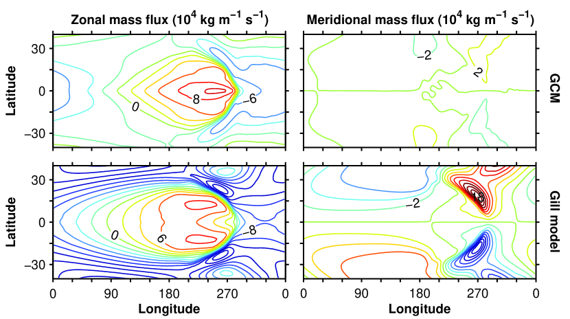
Figure 12: Zonal (left column) and meridional (right column) near-surface mass fluxes for the GCM (top row, averaged between the surface and $\sigma=0.73$ model level) and the Gill model forced by the GCM’s precipitation (bottom row, see Appendix for Gill model equations and parameters). The contour interval is $2\times 10^{4}\,\mathrm{kg\,m^{-1}\,s^{-1}}$.

There is a crescent-shaped region where the surface zonal wind is converging. This is where the precipitation (Fig. 2) and upward vertical velocity (Fig. 5) are largest. The horizontal scale of the convergence zone is similar to the equatorial Rossby radius, $(c/\beta)^{1/2}\sim 10^{\circ}$, where $\beta$ is the gradient of planetary vorticity and $c$ is the gravity wave speed (estimated using a characteristic tropospheric value for the Brunt-Väisälä frequency on the day side of the planet). The surface zonal wind can be qualitatively understood as the equatorially-trapped wave response to stationary heating: equatorial Kelvin waves propagate to the east of the heating and generate easterlies; equatorial Rossby waves propagate to the west of the heating and generate westerlies (Gill 1980).

The shape of the zero zonal wind line and its horizontal scale are similar to those of the Gill (1980) model, which describes the response of damped, linear shallow-water waves to a prescribed heat/mass source. For the prescribed heat source in the original Gill model, the crescent-shape zero zonal wind line extends over $\sim$2 Rossby radii and, as in the GCM simulation, is displaced to the east of maximum heating on the equator.

A complicating factor in the analogy between the GCM’s low-latitude surface winds and those of the Gill model is that the heating is prescribed in the Gill model, while it is interactive with the flow in the GCM. As previously mentioned, the precipitation is strongly shaped by the winds. To see if the analogy between the winds in the GCM and in the Gill model breaks down because of the more complex structure of the latent heating, we force a variant of the Gill model with the GCM’s precipitation field following the formulation of Neelin (1988) (see Appendix for details). The results of this calculation are compared with the GCM output in Fig. 12. The direction, large-scale structure, and, in the case of the zonal component, magnitude of the mass fluxes are similar between the GCM and precipitation-forced Gill model, though it is clear that there are quantitative differences.

In contrast to the larger-magnitude zonal wind, the meridional wind is diverging at the surface and converging aloft near the subsolar point (right panel of Fig. 11a,c). The dynamics of this are contained in the inviscid limit of the linear shallow-water equations: for a Sverdrup vorticity balance, the vortex stretching caused by the overall convergence near the surface near the equator must be balanced by moving poleward, toward higher planetary vorticity; hence the poleward meridional wind near the surface and the equatorward meridional wind aloft.

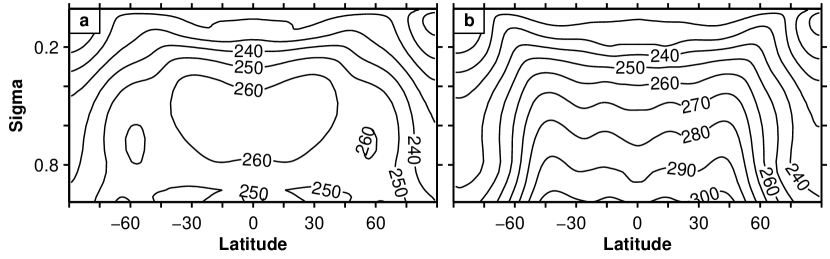
Figure 13: Temperature section of antisolar longitudes (a) and subsolar longitudes (b) of $\Omega_{E}$ simulation. Averages are taken over 10^∘ of longitude. The contour interval is $10\,\mathrm{K}$.

The Eulerian mean mass streamfunction (Fig. 6) has the opposite sense as Earth’s Hadley cells: in the zonal mean, there is descent on the equator, poleward flow near the surface, ascent near $15^{\circ}$, and equatorward flow in the mid-troposphere. If the dominant balance in the zonal momentum equation is between Coriolis acceleration and eddy angular momentum flux divergence, $-f\overline{v}\sim-\partial_{y}\overline{u^{\prime}v^{\prime}}$ (i.e., small local Rossby number as defined in Walker and Schneider (2006)), then the angular momentum flux convergence that establishes the superrotating zonal wind also leads to equatorward mean meridional wind in the free troposphere, as in Earth’s Ferrel cells (e.g., Held 2000). This can lead to a dynamical feedback that enhances superrotation (Schneider and Liu 2009): as superrotation emerges, the mean meridional circulation can change direction with a concomitant change in the direction of mean-flow angular momentum fluxes (changing from exporting angular momentum from the deep tropics to importing it), which enhances the superrotation.

The instantaneous, upper tropospheric zonal wind in the rapidly rotating simulation is shown in Fig. 7, and a corresponding animation is available at _anim. The large-scale features of the general circulation such as the high-latitude jets and divergent zonal wind in the tropical upper troposphere are clear in the instantaneous winds. The eddies in the animation generally have larger spatial scales and longer timescales than in the corresponding slowly rotating animation.

The vertically and globally integrated eddy kinetic energy is $1.0\times 10^{6}\ \mathrm{J\ m^{-2}}$. This is about 20% larger than int the slowly rotating case. The eddy kinetic energy spectrum has a typical, steep $n^{-3}$ shape to the smallest resolved wavenumber. In some sense, the integrated eddy kinetic energy belies the difference in synoptic variability between the rapidly and slowly rotating simulations: in the extratropics, for zonal wavenumbers between $\sim$3-6, the rapidly rotating simulation has a factor of 2-3 times more velocity variance (Fig. 8) than the slowly rotating simulation.

d Atmospheric stratification and energy transports

The tropospheric temperatures on the day side of the planet (Fig. 13) reflect the surface temperature variations: the temperature field has a local maximum near $\sim$40^∘ and is relatively uniform up to high latitudes (poleward of $\sim$50^∘). In the free troposphere on the day side, the lapse rates are close to the moist adiabatic lapse rate, computed using the local temperature and pressure, over a region roughly within the $300\,\mathrm{K}$ contour of the surface temperature. Note that $300\,\mathrm{K}$ does not have a particular physical significance—we are simply using it to describe a feature of the simulation. There is a local minimum of temperature on the equator which may be related to the downward vertical velocity there (Fig. 5). In low latitudes, there is a near-surface inversion on the night side of the rapidly rotating simulation that, as in the slowly rotating simulation, is the result of weak temperature gradients in the free troposphere and the small optical thickness of the atmosphere.

As in the slowly rotating simulation, the moist static energy flux divergence is positive on the day side and negative on night side of the planet (solid curves in Fig. 10); there is substantial cancellation between dry static energy and latent energy flux divergence near the subsolar point. Though the hydrological cycle is more active on the night side of the rapidly rotating simulation than in the slowly rotating simulation, the dry static energy component still dominates ($\gtrsim 80\%$) the moist static energy advection on the night side of the planet.

The two simulations are more similar in this respect than might have been anticipated given the differences in their flow characteristics, although there are regional differences that are obscured by averaging over latitude. The broad similarities can be understood by considering the moist static energy budget. In the time mean, denoted $\overline{(\cdot)}$, neglecting kinetic energy divergence and diffusive processes within the atmosphere, the mass-weighted vertical integral, denoted $\langle\cdot\rangle$, of the moist static energy flux divergence is balanced by surface energy fluxes, $F_{\mathrm{s}}$, and radiative tendencies, $Q_{\mathrm{rad}}$:

$$\nabla\cdot\langle\overline{{\bf u}h}\rangle=\overline{F}_{\mathrm{s}}+\overline{Q}_{\mathrm{rad}}.$$ (4.2)

As a result of the gross similarity of the two simulations in evaporation and low-latitude stratification (in part due to the smaller dynamical role that rotation plays near the equator) and hence the radiative cooling, the divergence of the moist static energy flux is also similar. In the extratropics, considering the sources and sinks of moist static energy does not provide a useful constraint because the stratification is dynamically determined (e.g., Held 1978; Schneider 2007) and there can be geostrophically balanced temperature gradients in rapidly rotating atmospheres; as result, the radiative cooling, through these dynamical influences on temperature, is determined by the flow, so the moist static energy flux divergence will not in general be independent of rotation rate. Indeed, the warm regions on the night side of the rapidly rotating simulation have larger moist static energy flux divergence than in those regions on the night side of the slowly rotating simulation as a result of the difference in circulation.

5 Conclusions

We have examined the dynamics of tidally locked, Earth-like planets. In particular, the dynamical regime of the atmosphere depends on the planet rotation rate, as anticipated from scaling arguments. The simulations demonstrate the importance of the atmospheric circulation in determining the surface climate. For example, the difference between the precipitation distributions in the slowly and rapidly rotating simulations clearly shows the dependence of the hydrological cycle on the circulation of the atmosphere. Interestingly, some aspects of the simulated climate are not sensitive to the planet’s rotation rate. In particular, the temperature contrast between the day and night side and evaporation rates are similar between the slowly and rapidly rotating simulations.

The general circulation of the slowly rotating atmosphere features global-scale, thermodynamically-direct, divergenct circulations with ascending motion at the subsolar point and descending motion elsewhere. In contrast, the general circulation of the rapidly rotating atmosphere features extratropical jets that owe their existence to rotational (Rossby) waves, and tropical surface winds that are the result of stationary equatorial (Rossby and Kelvin) waves. The isotropy of the winds in the slowly rotating regime and the anisotropy of the winds in the rapidly rotating regime are expected from the dominant balance of the horizontal momentum equations. Expectations for the free-atmospheric pressure and temperature gradients based on scale analysis were realized in the simulations of the different circulations regimes: temperature gradients are weak where Coriolis accelerations are weak (in low latitudes of the rapidly rotating atmosphere and globally in the slowly rotating atmosphere) and larger where Coriolis accelerations are dynamically important (in the extratropics of the rapidly rotating atmosphere).

While many aspects of the simulations can be explained by general circulation theories for Earth and Earth-like atmospheres, there remain quantitative questions that require more systematic experimentation than we have attempted here. For example, the dependence of the surface climate on the solar constant may be different from simulations with Earth-like insolation because of the differences in stratification.

Acknowledgments. Timothy Merlis was supported by a National Defense Science and Engineering Graduate fellowship and a National Science Foundation Graduate Research fellowship. We thank Sonja Graves for providing modifications to the GCM code and Simona Bordoni, Ian Eisenman, Andy Ingersoll, and Yohai Kaspi for comments on a draft of the manuscript. The simulations were performed on Caltech’s Division of Geological and Planetary Sciences Dell cluster. The program code for the simulations, based on the Flexible Modeling System of the Geophysical Fluid Dynamics Laboratory, and the simulation results themselves are available from the authors upon request.

6 Appendix: Gill model forced by precipitation

We use the formulation for a Gill model forced by precipitation (Neelin 1988), as opposed to the standard mass sink. The model equations are

$$-f\tilde{v} =-\partial_{x}\tilde{\phi}-\epsilon_{m}\tilde{u}$$ (6.1)

$$f\tilde{u} =-\partial_{y}\tilde{\phi}-\epsilon_{m}\tilde{v}$$ (6.2)

$$c^{2}(\partial_{x}\tilde{u}+\partial_{y}\tilde{v}) =-aP-\epsilon_{T}\tilde{\phi},$$ (6.3)

where $a=LR/c_{p}$ is the combination of the latent heat of vaporization, gas constant, and heat capacity at constant pressure that results from converting the precipitation rate to a temperature tendency in the thermodynamic equation and approximating Newtonian cooling by geopotential damping, $\epsilon_{m}$ is the Rayleigh drag coefficient of the momentum equations, $\epsilon_{T}$ is the damping coefficient for the geopotential, other variables have their standard meanings (e.g. $P$ is precipitation), and $\tilde{(\cdot)}=\int_{p_{b}}^{p_{s}}\ (\cdot)\ dp/g$ is the mass-weighted vertical integral over the boundary layer ($p_{b}$ is the pressure at the top of the boundary layer). We use fairly standard values for the constants (Table  1). The qualitative aspects of the solutions that we discuss are not sensitive to these choices.

constant	value
c	50 m s-1
$\beta$	2.22 $\times 10^{-11}$ m-1 s-1
$\epsilon_{m}$	(1 day)-1
$\epsilon_{T}$	(20 day)-1
a	7.14 $\times 10^{5}$ J kg-1

Table 1: Gill model constants and their values.

The three equations can be combined into a single equation for $\tilde{v}$:

$$\begin{split}[-\epsilon_{T}(\epsilon_{m}^{2}+\beta^{2}y^{2})/c^{2}+\epsilon_{m}(\partial_{xx}+\partial_{yy})+\beta\ \partial_{x}]\tilde{v}=\\ -(\epsilon_{m}\partial_{y}-\beta y\ \partial_{x})\ aP/c^{2},\end{split}$$ (6.4)

where $\beta$-plane geometry ($f=\beta y$) has been assumed. The boundary value problem for $\tilde{v}$ is discretized by Fourier tranforming in the x-direction and finite differencing in the y-direction. It is solved using the GCM’s climatalogical precipitation field on the right-hand side (Fig. 2).

References

- Charbonneau et al. (2009) Charbonneau, D., and Coauthors, 2009: A super-Earth transiting a nearby low-mass star. Nature, 462, 891–894.
- Charbonneau et al. (2000) Charbonneau, D., T. M. Brown, D. W. Latham, and M. Mayor, 2000: Detection of planetary transits across a Sun-like star. Astrophys. J., 529, L45–L48.
- Charney (1963) Charney, J. G., 1963: A note on large-scale motions in the Tropics. J. Atmos. Sci., 20, 607–609.
- Frierson (2007) Frierson, D. M. W., 2007: The dynamics of idealized convection schemes and their effect on the zonally averaged tropical circulation. J. Atmos. Sci., 64, 1959–1976.
- Frierson et al. (2006) Frierson, D. M. W., I. M. Held, and P. Zurita-Gotor, 2006: A gray-radiation aquaplanet moist GCM. Part I: Static stability and eddy scale. J. Atmos. Sci., 63, 2548–2566.
- Gill (1980) Gill, A. E., 1980: Some simple solutions for heat induced tropical circulation. Quart. J. Roy. Meteor. Soc., 106, 447–462.
- Hartmann (1994) Hartmann, D., 1994: Global Physical Climatology. Academic Press, 411 pp.
- Held (1978) Held, I. M., 1978: The tropospheric lapse rate and climatic sensitivity: Experiments with a two-level atmospheric model. J. Atmos. Sci., 35, 2083–2098.
- Held (2000) Held, I. M., 2000: The general circulation of the atmosphere. Proc. Program in Geophysical Fluid Dynamics, Woods Hole Oceanographic Institution, Woods Hole, MA. URL https://darchive.mblwhoilibrary.org/handle/1912/15.
- Held and Hou (1980) Held, I. M., and A. Y. Hou, 1980: Nonlinear axially symmetric circulations in a nearly inviscid atmosphere. J. Atmos. Sci., 37, 515–533.
- Hide (1969) Hide, R., 1969: Dynamics of the atmospheres of the major planets with an appendix on the viscous boundary layer at the rigid bounding surface of an electrically-conducting rotating fluid in the presence of a magnetic field. J. Atmos. Sci., 26, 841–853.
- Hubbard (1984) Hubbard, W. B., 1984: Planetary Interiors. Van Nostrand Reinhold Co., 334 pp.
- Joshi (2003) Joshi, M., 2003: Climate model studies of synchronously rotating planets. Astrobiology, 3, 415–427.
- Joshi et al. (1997) Joshi, M. M., R. M. Haberle, and R. T. Reynolds, 1997: Simulations of the atmospheres of synchronously rotating terrestrial planets orbiting M Dwarfs: Conditions for atmospheric collapse and the implications for habitability. Icarus, 129, 450–465.
- Neelin (1988) Neelin, J. D., 1988: A simple model for surface stress and low-level flow in the tropical atmosphere driven by prescribed heating. Quart. J. Roy. Meteor. Soc., 114, 747–770.