Quantum Persistence: A Random Walk Scenario

Abstract

In this paper we extend the concept of persistence, well defined for classical stochastic dynamics, to the context of quantum dynamics. We demonstrate the idea via quantum random walk and a successive measurement scheme, where persistence is defined as the time during which a given site remains unvisited by the walker. We also investigated the behavior of related quantities, e.g., the first-passage time and the succession probability (newly defined), etc. The study reveals power law scaling behavior of these quantities with new exponents. Comparable features of the classical and the quantum walks are discussed.

Persistence in classical dynamical systems is a topic which has been extensively studied during the recent years satya . The persistence probability ($P_{cl}(t)$) that the order parameter in a magnetic system has not changed sign till time $t$ derrida and the persistence of unvisited sites in a diffusion problem bray are common examples which have received a lot of attention. The importance of persistence phenomena lies in the fact that the persistence probability in many systems shows an algebraic decay (in time) with an exponent not related to any other known static or dynamical exponents.

The dynamics of a quantum system is expected to be different from the corresponding classical counter part, yet investigating persistence behavior in the quantum case has remained an interesting open problem till date. However, defining quantum persistence is ridden with the fundamental problem of measurement, since in order to ensure whether or not the system persisted in a given state (or in a chosen subspace ${\mathbf{X}}$), one has to impose a continuous monitoring which would change the dynamics of a quantum system in some essential way. Hence in the quantum case, meaningful definition of persistence has to include the associated measurement scheme (i.e., how the evolution is disturbed by the measurement), and should essentially be dependent on that. The dynamical process we consider here is a discrete quantum random walk (QRW) aharonov ; nayak1 ; amban ; kempe . Classical random walk (CRW) on a line is a much studied topic chandra ; book ; redner where at every step one tosses a fair coin and takes a step, either to the left or right. The unitary implementation of QRW may be achieved through coupling an additional degree of freedom (a quantum coin) with the walker. This coin degree of freedom is called the chirality, which takes values “left” and “right”, analogous to Ising spin states $\pm 1$, and directs the motion of the particle. The state of the walker is expressed in the $|x\rangle|d\rangle$ basis, where $|x\rangle$ is the position (in real space) eigenstate and $|d\rangle$ is the chirality eigen state (either “left” or “right, denoted by $|L\rangle$ and $|R\rangle$ respectively). There may be several ways of choosing the unitary operator causing the rotation of the chirality state, conventional choice effecting the rotation of the chirality state is the Hadamard coin nayak1 ; amban ; kempe unitary operator. (Most of the results are, however, believed to be coin independent.) The rotation is followed by a translation represented by the operator $T$:

$$\begin{array}[]{l}T|x\rangle|L\rangle\rightarrow|x-1\rangle|L\rangle\\ T|x\rangle|R\rangle\rightarrow|x+1\rangle|R\rangle\\ \end{array}.$$ (1)

The two component wave function $\psi({x},t)$ describing the position of the particle is written as

$$\psi({x},t)=\begin{pmatrix}\psi_{L}({x},t)\\ \psi_{R}({x},t)\end{pmatrix},$$ (2)

and the occupation probability of site $x$ at time $t$ is given by

$$f({x},t)=|\psi_{L}({x},t)|^{2}+|\psi_{R}({x},t)|^{2};$$ (3)

normalization implying $\sum_{x}f({x},t)=1$.

In the case of the classical random walker, two well studied quantities are persistence or the survival probability $P_{cl}({x},t)$ defined as the probability that the site at $x$ has not been visited till time $t$ chandra ; book and the first passage time $F_{cl}({x},t)$ which is the probability that the walker has reached the site $x$ for the first time at time $t$ redner . The two quantities are related by

$$F_{cl}({x},t)=-\frac{\partial P_{cl}({x},t)}{\partial t}.$$ (4)

At $t>>1$, both the persistent probability and first passage probabilities decay algebraically in time with exponents $\alpha_{cl}$ and $\beta_{cl}$ which obey the relation

$$\alpha_{cl}=\beta_{cl}-1,$$ (5)

consistent with the equality in (4). We are primarily interested in the analogues of these two quantities in the QRW.

We now define our measurements schemes and the observables to quantify the concept of quantum persistence in this case. In order to measure persistence in strict sense, one is left with no other choice than to monitor the system continually over time. One way of achieving this is to impose a direct time-continual projective measurement that determines at every moment whether or not the system persists within the subspace ${\mathbf{X}}$ in question. In this discrete time version of quantum walk, this amounts to carrying out a measurement after every time step of the unitary evolution following the scheme described below. The walk starts from some given site at $t=0$, and a detector is placed at some other given site $\bar{x}$, which detects the particle with probability unity if it reaches there. If the particle is detected at $\bar{x}$, the evolution is stopped (here, ${\mathbf{X}}$ is the entire lattice excluding $\bar{x}$). Now the question asked for such a system (rather, for an ensemble of such systems), is what is the probability that the detector does not click till time $t$. This is the persistence probability $P({\bar{x}},t)$. It is equivalent to carrying out measurements at the site $\bar{x}$ after each step of unitary evolution of the ensemble and calculating the probability from the fraction of the surviving copies (for which $\bar{x}$ is yet unvisited) at each step. Within this setup of QRW on a line, placing the detector at $\bar{x}$ amounts to having a semi infinite walk (SIW) amban ; absorb1 ; bach ; Kiss with an absorbing boundary at $\bar{x}$ and an open end in the other direction. Let us give a concrete illustration of the scheme with a detector placed at $\bar{x}=1$. Suppose the walker starts at $x=0$ with left chirality. At time $t=1$ in fifty percent cases it will be detected at $\bar{x}$ and the time evolution will be stopped. Persistence probability is therefore $1/2$ for $\bar{x}$ at $t=1$. The remaining fifty percent walks will evolve unitarily to the next step $t=2$. At $t=3$, the normalized probabilities at $x=-3$, $x=-1$ and $x=1$ are equal to 1/4, 1/2 and 1/4 respectively (and zero elsewhere). Hence now the detector detects the walker at $\bar{x}$ with probability 1/4, which means the 3/4 fraction of the population that was carried over to $t=2$ would be carried over to the next time step at $t=3$. This is $3/8$ of the initial population (at $t=0$). Hence the persistence probability at $t=3$ will be $3/8$ for $\bar{x}=1$.

At each time step the ensemble is measured, and the amplitudes describe only to the surviving copies, and the probabilities are to be renormalized. Let the normalized occupation probability at $x$ at time $t$ be denoted by $\tilde{f}(x,t)$. Thus $\tilde{f}(\bar{x},t^{\prime})$ denotes the fraction of the copies that survived the measurement at time $t^{\prime}-1$ (not the fraction of the initial population) which reaches $\bar{x}$ at time $t^{\prime}$. The persistence probability is hence given by

$$P_{SIW}({\bar{x}},t)=\prod_{t^{\prime}=1}^{t}(1-\tilde{f}({\bar{x}},t^{\prime})).$$ (6)

It is to be mentioned here that by placing the detector at $\bar{x}$, it is possible to find the occupation probabilities for all $x$ and $t$ (which are strongly dependent on $\bar{x}$) but the persistent probability is obtained only for $x=\bar{x}$. One may define a first passage time $F_{SIW}({\bar{x}},t)$ analogous to the classical random walk in this case as follows:

$$F_{SIW}({\bar{x}},t)=\prod_{t^{\prime}=1}^{t-1}(1-\tilde{f}({\bar{x}},t^{\prime}))\tilde{f}({\bar{x}},t)$$ (7)

$$=P_{SIW}({\bar{x}},t-1)\tilde{f}({\bar{x}},t).$$

It may be mentioned here that some related studies have been made earlier absorb1 ; bach and the problem of persistence measured in this way had been addressed with the boundary kept far from the starting point of the walker bach .

As mentioned before, definition of quantities in a quantum system depend heavily on the measurement scheme and we next pose similar interesting and well defined questions that brings out the more intrinsic characteristics of the dynamics somewhat directly, by monitoring what we call the succession probability $S({\mathbf{X}},t)$ defined as follows. Let us consider a system allowed to evolve unitarily from a given initial state at $t_{i}=0$, up to a terminating time $t^{\prime}=\Delta t$, when finally a measurement is done on it in order to determine whether or not it resides at a given state (or within a subspace) ${\mathbf{X}}$ and the evolution is stopped (e.g., in the QRW, one discards the walk). The entire process is repeated for increasing terminating times: $t^{\prime}=\Delta t,2\Delta t,3\Delta t,...t$. Now the question is asked, what is the probability that the system will be found within ${\mathbf{X}}$ in every measurement with $t^{\prime}\leq t$.

For a continuous-time evolution, this probability will be called the succession probability $S({\mathbf{X}},t)$ in the limit $\Delta t\rightarrow 0$. For a discrete random walk, $\Delta t$ will correspond to a single step. For example, in the context of QRW, one might choose to calculate the probability of a random walker not being found at some target site $\bar{x}$ in the successive measurements done at $t^{\prime}=1,2...t$ (starting from a given site). The subspace ${\mathbf{X}}$ in this case is constituted of all lattice points the walk may include, excluding $\bar{x}$ and we may then use the notation $S(\bar{x},t)$ to denote the succession probability. It may be noted that in the classical case, one need not restart the evolution, after each measurement, since the measurement would not disturb it. $S({\bar{x}},t)$ clearly differs from $P_{cl}({\bar{x}},t)$ in general, since in case of $S({\bar{x}},t)$, in calculating the probability of finding the system within ${{\mathbf{X}}}$ at $t^{\prime}$, one takes contributions of all the paths running from the initial time 0 up to the final time $t^{\prime}$, including those which went out of ${{\mathbf{X}}}$ in the intermediate times.

In the present one dimensional setting this amounts to allowing the system to evolve unitarily in either direction (infinite walk or IW nayak1 ) for an interval $t^{\prime}$, when the measurement is done and the walk is discarded. We choose, again, ${\mathbf{X}}$ to be the entire lattice except a given point $x={\bar{x}}$, where we would like to see whether the particle has reached or not. To determine $S({\bar{x}},t)$ for a given $t$, the termination time $t^{\prime}$ is varied as $t^{\prime}=1,2...t$, and for each given $t^{\prime}$ one determines the occupation probability $f({\bar{x}},t^{\prime})$ and calculates $S({\bar{x}},t)$ as:

$$S({\bar{x}},t)=\prod_{t^{\prime}=1}^{t}(1-f({\bar{x}},t^{\prime})).$$ (8)

An analogue of the the first passage time may also be defined as

$$F_{IW}({\bar{x}},t)=\prod_{t^{\prime}=1}^{t-1}(1-f({\bar{x}},t^{\prime}))f({\bar{x}},t)$$ (9)

$$=S({\bar{x}},t-1)f({\bar{x}},t).$$

Experimentally this corresponds to simply knowing $f({\bar{x}},t^{\prime})$ for $t^{\prime}\leq t$.

Some time dependent features in this type of infinite walk have been studied like the hitting time, recurrence time, Polya number etc. hitting1 ; hitting2 ; Stefanak1 ; Stefanak2 , which involve the first passage time. However, in these studies, the spatial dependence has not been considered. For example, quantities like first passage time specifically at the origin has been estimated.

It is important to note here that the quantities $S$ and $P_{SIW}$ given by equations (8) and (6) (as also $F_{IW}$ and $F_{SIW}$) are identical in form: the difference being $f$ appearing in the infinite walk in place of $\tilde{f}$ in the semi infinite walk. Thus $f$ and $\tilde{f}$ essentially make these quantities different. As an example, we have shown $f(x,t)$ and $\tilde{f}(x,t)$ as functions of $x$ at a fixed time $t$ in Fig 1. For the semi infinite walk, there is a detector placed at $x=10$. To emphasize the difference, we have generated a walk biased towards the right, and the unbounded walk shows it clearly. On the other hand, in the semi infinite walk, the walker is not allowed beyond $x=10$ and consequently is driven towards the left. Obviously, even if a walk with symmetric boundary condition is initiated, the presence of the detector will convert it to a asymmetric walk.

In the calculation, a quantum random walk is initialized at the origin with $\psi_{L}(0,0)=a_{0},\psi_{R}(0,0)=b_{0};~{}~{}a_{0}^{2}+b_{0}^{2}=1.$ (All other $\psi_{L}$ and $\psi_{R}$ taken equal to zero). $\psi_{L}({\bar{x}},t)$ and $\psi_{R}({\bar{x}},t)$ are recursively evaluated for all $x$ and $t$. In the bounded (semi infinite) walk, contributions from the walks going through $\bar{x}$ are ignored. Unless otherwise specified, we have taken $a_{0}=1/\sqrt{2},b_{0}=i/\sqrt{2}$ which would result in a symmetric walk for the unbounded (infinite) walk case.

The results for SIW are essentially numerical; the persistence probabilities here saturate in time. This saturation behavior apparently originates from the simultaneous effect of drifting of the quantum walker away from the origin and the presence of the boundary at $\bar{x}$. These observations are in agreement with bach and consistent with other results involving recurrence time etc. amban ; Kiss . The first passage times, on the other hand, decay algebraically with $t$. As already mentioned, in bach , the persistence probability for large $\bar{x}$ was found to vary as

$$P_{SIW}({\bar{x}},t)=P_{0}+{\rm{const}}(t/{|\bar{x}|})^{-\alpha_{SIW}}$$ (10)

where $P_{0}$ is the saturation value and $\alpha_{SIW}=2$. We verify this result with the observation that $P_{0}$ has a weak dependence on $\bar{x}$ and observe that the numerical value of $\alpha_{SIW}$ approaches the value 2 asymptotically. The numerically estimated values of $P_{0}(\bar{x})$ are found to vary as $(a-b\exp(-c\bar{x}))$ with $c=0.30\pm 0.02$, shown in the inset of Fig 2. Using these values of $P_{0}(\bar{x})$, we show that a data collapse is obtained when the residual persistence probability $P_{SIW}({\bar{x}},t)-P_{0}(\bar{x})$ is plotted against $t/|\bar{x}|$. The first passage time $F_{SIW}({\bar{x}},t)$ behaves as

$$F_{SIW}({\bar{x}},t)\propto(t/|{\bar{x}}|)^{-\beta_{SIW}}/|{\bar{x}}|,$$ (11)

with $\beta_{SIW}\simeq 3.0$. Results for the collapsed data of persistence and first passage times are shown in Figs 2 and 3.

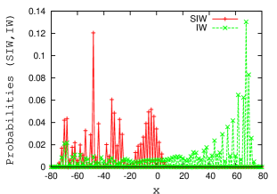
Figure 1: (Color online) Comparison of the probabilities $\tilde{f}(x,t)$ for the semi infinite walk (SIW) and $f(x,t)$ for the infinite walk (IW) at time $t$ = 100: in the IW probabilities extend to both sides, in the SIW (with a detector placed at ${\bar{x}}=10$), the particle is not found beyond $x=10$.

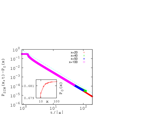
Figure 2: (Color online) The data collapse for the residual persistence probability in the quantum random walk shown for different values of $x=\bar{x}$. The straight line in the log-log plot has the slope = -2.0. Inset shows the variation of the saturation value $P_{0}$ with $x$.

For the unbounded or infinite walk, the calculations can also be done using the analytical forms available in nayak1

$$\psi_{L}({x},t)=\frac{1+(-1)^{x+t}}{2}\int\frac{dk}{2\pi}(1+\frac{\cos k}{\sqrt{1+\cos^{2}k}})e^{-i(\omega_{k}t+kx)}$$ (12)

$$\psi_{R}({x},t)=\frac{1+(-1)^{x+t}}{2}\int\frac{dk}{2\pi}\frac{e^{ik}}{\sqrt{1+\cos^{2}k}}e^{-i(\omega_{k}t+kx)}$$ (13)

(which are obtained for a initial state with left chirality, i.e., $a_{0}=1,b_{0}=0$) and evaluate $f({\bar{x}},t)$ directly by numerical integration.

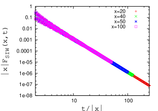
Figure 3: (Color online) The data collapse for the first passage probability in the quantum random walk shown for different values of $x=\bar{x}$. Fitted straight line has slope = -3.0.

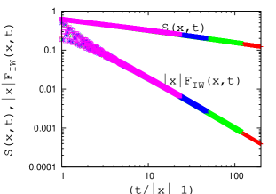
Figure 4: (Color online) The data collapse for the succession probability and scaled first passage probability defined for a infinite quantum random walk shown for different values of $x=10$ (red), $20$ (green), $50$ (blue), $100$ (magenta).

Power law decay for both $S({\bar{x}},t)$ and $F_{IW}({\bar{x}},t)$ are observed:

$$S({\bar{x}},t)\propto(t/|{\bar{x}}|-1)^{-\alpha_{IW}}$$ (14)

for $t/|{\bar{x}}|>1$, and

$$F_{IW}({\bar{x}},t)\propto(t/|{\bar{x}}|-1)^{-\beta_{IW}}/|{\bar{x}}|$$ (15)

for $t/|{\bar{x}}|>>1$ with $\alpha_{IW}\simeq 0.31$ and $\beta_{IW}\simeq 1.31$. Data collapse for $S({\bar{x}},t)$ and $F_{IW}({\bar{x}},t)$ from the numerical evolution of the infinite walk are shown in Fig. 4. These results are obtained with $a_{0}=1/\sqrt{2},b_{0}=i/\sqrt{2}$ which correspond to a symmetric walk. Results obtained from the numerical integration of Eqs. 12 and 13 (corresponding to $a_{0}=1,b_{0}=0$ giving an asymmetric walk) show the same scaling behaviour as $S({\bar{x}},t)$ and $F_{IW}({\bar{x}},t)$. Thus the exponents are independent of the initial conditions as expected.

As discussed in Stefanak1 ; Stefanak2 , the quantum walk on a line is recurrent, i.e. it returns to the origin with certainty and the same applies to visiting any other lattice point. Hence, the asymptotic succession probability is zero, which is in agreement with the power law decay of $S(\bar{x},t)$ found in the present paper.

While the exponents $\alpha_{IW}$ ($\alpha_{SIW}$) and $\beta_{IW}$ ($\beta_{SIW}$) are different from the classical $\alpha_{cl}$ and $\beta_{cl}$, they enjoy a relationship identical to eq (5). We consider some other quantities related to the function $F_{IW}(x,t)$ which one can compare with their classical counterparts. Plotting $F_{IW}(x,t)$ against $x$ or $t$, we notice that it has an oscillatory behavior. These oscillations which die down for large values of $t/x$ as is apparent from Fig. 4 can be traced to the oscillatory behavior of $f(x,t)$ for a QRW observed earlier nayak1 ; amban ; kempe . From Figs 5 and 6, we observe that $F_{IW}(x,t)$ actually attains a maximum value $F_{IW,max}(x,t)$ at values of $|x|=x_{max}$ (or $t=t_{max}$) for fixed values of $t$ (or $x$). We notice that $F_{IW,max}(x_{max},t)\propto x_{max}^{-\delta}$ where $\delta\simeq 0.59$. Keeping $x$ fixed, $F_{IW,max}(x,t_{max})$ versus $t_{max}$ shows the same kind of dependence, i.e., $F_{IW,max}(x,t_{max})\propto t_{max}^{-\delta}$. That the scalings with $t_{max}$ and $x_{max}$ turn out to be identical is not surprising as $x$ scales as $t$ in a QRW. It is not possible to obtain this scaling form directly from eq. (15) since $F(x,t)$ attains a maximum value when $t/|x|$ is close to unity where the fitted scaling form is not exactly valid. In fact, eq. (15) does not give any maximum value at all.

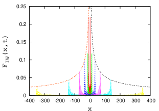
Figure 5: Typical variation of $F_{IW}(x,t)$ against $x$ for different values of $t=10,20,50,100,200,500$. The curves extend over larger values of $x$ as $t$ is increased. The peaks are approximately fitted to $0.81x_{max}^{-0.59}$.

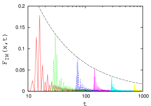
Figure 6: Typical variation of $F_{IW}(x,t)$ against $t$ for different values of $x=10,20,50,100,200,500$. The curves extend over larger values of $t$ as $x$ is increased. The peaks are approximately fitted to $t_{max}^{-0.59}$.

Another dynamic quantity called hitting time has been estimated earlier for the QRW, in which an absorber is assumed to be located at a specific vertex of a hypercube within which the walk is conceived hitting1 ; hitting2 . The average hitting time is by definition the average time to reach that particular vertex for the first time. One can evaluate the average hitting time $\tau_{h}(x)$ in the infinite walk scheme using $\tau_{h}(x)=\sum_{0}^{T}tF_{IW}(x,t)$ where $t$ is allowed to vary from $0$ to $T$:

$$\tau_{h}\approx\int_{0}^{T}tF_{IW}(x,t)dt$$

$$\sim{T}^{2-\beta_{IW}}x^{\beta_{IW}-1}/(2-\beta_{IW})+O({T}^{-{\beta_{IW}+1}}).$$

The numerical data (not shown) gives a fairly good agreement with this scaling. The above equation shows that $\tau_{h}$ blows up for $T\to\infty$ in agreement with some earlier results using other coins hitting1 ; hitting2 .

We thus observe that a number of quantities related to the dynamics of a quantum random walker follow power law behavior with time. Of these, the persistence probability $P_{SIW}(\bar{x},t)$, which is obtained from a semi infinite walk, is drastically different from its classical analogue as it approaches a constant value in a power law fashion with an exponent which is quite different from the classical value 1/2. The first passage time also has a power law decay with a new exponent. The numerical data also indicate that the two quantities obey a simple relation as in the classical case (eq (4)).

A different quantum measure which we call the succession probability has been proposed and calculated in the present work and a corresponding first passage probability defined. These measures can be obtained from an infinite walk. The persistence probability and succession probabilities are similar in form but the results are highly different with the succession probability exhibiting a power law decay (no saturation) with yet another new exponent. However, the form of the probabilities in eqs (10), (11) and (14), (15) and the values of the exponents indicate the validity of eq (4) in the quantum case as well.

In a classical random walk, $\langle x^{2}\rangle\propto t^{\gamma_{cl}}$ with $\gamma_{cl}=1$ and in one dimension this scaling governs all other dynamic behavior including persistence. Thus all other exponents like $\alpha_{cl}$ and $\beta_{cl}$ are essentially dependent on $\gamma$, e.g., $\alpha_{cl}=\gamma_{cl}/2$ and $\beta_{cl}=\frac{3}{2}\gamma_{cl}$. A quantum walker propagates much faster; here $\langle x^{2}\rangle\propto t^{\gamma_{q}}$ with $\gamma_{q}=2$. Thus the dimensionless factor $x/t$ appears in the scaling argument of the dynamic quantities. The exponents $\alpha_{SIW}\simeq 2$ and $\beta_{SIW}\simeq 3$ appear to be simply related to $\gamma_{q}$; $\alpha_{SIW}=\gamma_{q}$ and $\beta_{SIW}=\frac{3}{2}\gamma_{q}$ showing that here too the persistence phenomena is governed by the scaling $\langle x^{2}\rangle\propto t^{\gamma_{q}}$ only.

For the infinite walk case, the exponents $\alpha_{IW}$ and $\beta_{IW}$ are apparently not simply related to $\gamma_{q}$. We have estimated some additional quantities involving the first passage time. The maximum values of the classical probability $F_{cl}$, behaves as $1/t_{max}$ (for $x$ constant) or $1/x_{max}^{2}$ (for $t$ constant) showing that the obtained exponents are simple multiples of $\gamma_{cl}=1$. On the other hand, the behavior of $F_{IW,max}$ appears to depend on the value of $\alpha_{IW}$ and not $\gamma_{q}$ as it varies with ${t_{max}}$ or $x_{max}$ with an exponent $\delta$ which is very close to $2\alpha_{IW}$ numerically.

The average hitting time for a CRW is found to vary as $T^{\gamma_{cl}/2}$. In the infinite QRW, this variation is given by $T^{2-\beta_{IW}}$. For the classical case, $2-\beta_{cl}=\gamma_{cl}/2$ but since no such relation exists for the quantum case, the hitting time scaling is therefore not dictated by $\gamma_{q}$ but by $\beta_{IW}$ (or $\alpha_{IW}$) only.

Lastly, it is true that the probabilities $\tilde{f}({\bar{x}},t)$ are quite different from $f({\bar{x}},t)$ making the persistence and succession probabilities distinct, however, the feature that the quantum walker walks away from the origin (in contrast to a classical walker) is present in both. This makes the persistence probability and the succession probabilities quite large in magnitude compared to classical persistence probabilities. For the quantum persistence probability, $P_{SIW}$, the additional constraint of the presence of the boundary makes it saturate.

Acknowledgment: Financial supports from DST grant no. SR-S2/CMP-56/2007 (PS) and UGC sanction no. UGC/209/JRF(RFSMS) (SG) are acknowledged.

References

- (1)
- (2) S.N. Majumdar, Curr. Sci. 77, 370 (1999).
- (3) B. Derrida, A.J.Bray and C. Godreche, J.Phys. A 27, L357 (1994).
- (4) S. J. O’Donoghue and A. J. Bray, Phys. Rev. E 64, 041105 (2001); P. K. Das, S. Dasgupta and P. Sen, J. Phys. A: Math. Theor. 40, 6013 (2007).
- (5) S. Chandrasekhar, Phys. Rev. 15, 1 (1943).
- (6) G. H. Weiss, Aspects and applications of the random walk, North Holland, Amsterdam, 1994.
- (7) S. Redner, A guide to first-passage processes, Cambridge University Press, 2001.
- (8) Y. Aharonov, L. Davidovich and N. Zagury, Phys. Rev. A 48, 1687 (1993).
- (9) A. Nayak and A. Vishwanath, DIAMCS Technical Report 2000-43 and Los Alamos preprint archive,quant-ph/0010117.
- (10) A. Ambainis, E. Bach, A. Nayak, A. Vishwanath and J. Watrous, Proc. 33th New York, NY (2001).
- (11) J. Kempe, Contemporary Physics 44, 307 (2003).
- (12) T. Yamasaki, H. Kobayashi, and H. Imai, arxiv: quant-ph/0205045.
- (13) E. Bach, S. Coppersmith, M. Paz Goldshen, R. Joynt and J. Watrous, Journal of Computer and Systems Sciences, 69, 562 (2004).
- (14) T. Kiss, L. Kecskes, M. Stefanak, I. Jex, Physica Scripta T135, 014055 (2009).
- (15) J. Kempe, Proc. 7th RANDOM, 354 (2003); J. Kempe, Probability Theory and Related Fields, 133, 215 (2005).
- (16) H. Krovi and T.A. Brun, Phys. Rev. A 73, 032341 (2006).
- (17) M. Stefanak, I. Jex, T. Kiss, Phys. Rev. Lett 100, 020501 (2008).
- (18) M. Stefanak, T. Kiss and I. Jex, Phys. Rev. A 78, 032306 (2008).