Laser-induced nonsequential double ionization at and above the recollision-excitation-tunneling threshold

Abstract

We perform a detailed analysis of the recollision-excitation-tunneling (RESI) mechanism in laser-induced nonsequential double ionization (NSDI), in which the first electron, upon return, promotes a second electron to an excited state, from which it subsequently tunnels, based on the strong-field approximation. We show that the shapes of the electron momentum distributions carry information about the bound-state with which the first electron collides, the bound state to which the second electron is excited, and the type of electron-electron interaction. Furthermore, one may define a driving-field intensity threshold for the RESI physical mechanism. At the threshold, the kinetic energy of the first electron, upon return, is just sufficient to excite the second electron. We compute the distributions for helium and argon in the threshold and above-threshold intensity regime. In the latter case, we relate our findings to existing experiments. The electron-momentum distributions encountered are symmetric with respect to all quadrants of the plane spanned by the momentum components parallel to the laser-field polarization, instead of concentrating on only the second and fourth quadrants.

I Introduction

Electron-electron correlation in strong laser fields has raised considerable interest for over a decade, in particular in the context of laser-induced nonsequential double and multiple ionization Electron correlation . Concrete examples are the early measurements of a “knee” in the double ionization yield as a function of the laser-field intensity, which deviates from the predictions of sequential models in orders of magnitude knee , and the peaks in the electron momentum distributions in nonsequential double ionization (NSDI), as functions of the electron components $p_{n\parallel}$ $(n=1,2)$ parallel to the laser-field polarization Weber . Such peaks occur at nonvanishing parallel momenta and cannot be explained by a sequential mechanism.

Presently, it is an established fact that NSDI occurs due to the inelastic recollision of an electron with its parent ion tstep . In this recollision, the first electron gives part of the kinetic energy it acquired from the driving field to a second electron, which is then freed.

The simplest type of recollision which can lead to this phenomenon is electron-impact ionization. Thereby, the first electron, upon return, provides the second electron with enough energy so that it is able to overcome the second ionization potential of the target in question and reach the continuum. Both electrons leave simultaneously and lead to distributions peaked at nonvanishing momenta, occupying the first and third quadrant of the plane $p_{1\parallel}$$p_{2\parallel}$ spanned by the parallel momentum components.

Electron-impact ionization is possibly the most extensively investigated NSDI mechanism NSDIsfa ; Carla1 ; Carla2 ; Carla3 ; scatteringtdse ; experimentsV ; Emanouil ; prauzner ; Denys . This is due to the fact that, until the past few years, it was sufficient to describe key features observed experimentally in the electron momentum distributions. Concrete examples are the peaks near the non-vanishing momenta $p_{1\parallel}=p_{2\parallel}=\pm 2\sqrt{U_{p}}$, where $U_{p}$ is the ponderomotive energy, and the recently reported V-shaped structure experimentsV , which is a signature of the long-range character of the electron-electron interaction Carla2 ; Emanouil ; prauzner ; Denys ; scatteringtdse . Moreover, from the theoretical viewpoint, this mechanism is considerably easier to model, as compared to other rescattering processes. This is particularly true in the context of semi-analytical models, such as the strong-field approximation NSDIsfa ; Carla1 ; Carla2 ; Carla3 ; Kopold ; Denys .

Recent experimental results, however, reveal other rescattering mechanisms apart from electron-impact ionization. For instance, if the driving-field intensity is below the threshold intensity, the kinetic energy of the recolliding electron is no longer sufficient to make the second electron overcome the ionization potential of the singly ionized core and reach the continuum Eremina ; threshold . In this intensity range, the energy transferred to the core is only enough to raise the second electron to an excited bound state, from which it subsequently tunnels. This process is known as recollision-excitation-tunneling ionization (RESI). This mechanism is also important for specific targets, such as argon Jesus , even if intensities above the threshold are taken, provided the driving pulse is long enough.

For this specific mechanism, the first electron leaves near a crossing of the driving field, whilst the second electron is freed near a field maximum. The time delay between both electrons suggests that they leave with opposite momenta. This implies that the second and the fourth quadrant of the $p_{1\parallel}$$p_{2\parallel}$ plane are expected to be populated timelag . A population in such regions of the parallel momentum plane has also been observed for NSDI of diatomic molecules, especially if the molecules in question are aligned perpendicular to the laser-field polarization NSDIalign ; Chen ; Baierexcited ; Prauznerexc . Furthermore, it has been recently shown that electron-impact ionization, alone, would not be very useful for retrieving the molecular structure in the experimentally relevant intensity range UCL2008 . All these examples suggest that the RESI mechanism is becoming increasingly important, in view of the driving field intensities and targets employed.

This mechanism, however, is considerably less understood than electron-impact ionization. In fact, apart from early results in which only the RESI yield has been calculated within a semi-analytical framework Kopold , most existing results are the outcome of computations, either classical Prauznerexc ; Chen ; timelag ; Agapi09 ; otherclassical or quantum mechanical Baierexcited , for which the different rescattering mechanisms cannot be easily disentangled.

In previous work SF2009 , we have studied the RESI physical mechanism, within the strong-field approximation. In this framework the transition amplitude is written as a multiple integral, with a time-dependent action and slowly-varying prefactors. This approach has the particular advantage of providing a clear space-time picture of the process in question, in terms of electron trajectories, while retaining features such as quantum-interference effects Orbits .

We have shown that the RESI mechanism may be understood as the combination of two processes. For the first electron, a behavior similar to rescattered above-threshold ionization is present. The main difference lies on the fact that part of the kinetic energy of the first electron is given to the parent ion. This leads to a maximal kinetic energy slightly smaller than the high-order ATI cutoff $10U_{p}.$ The second electron, which is tunnel ionized at a subsequent time, behaves in the same way as in direct above-threshold ionization. Hence, its maximal kinetic energy is given by the direct ATI cutoff, i.e., $2U_{p}.$ This allowed one to determine kinematic constraints for the RESI mechanism, which lead to distributions which equally occupy the four quadrants of the $p_{1\parallel}p_{2\parallel}$ plane. For an early derivation of somewhat different kinematic constraints for this mechanism see, e.g., Ref. Constraints .

In the above-stated investigations, however, we assumed the prefactors in the strong-field approximation amplitude to be constant. Nonetheless, in a more realistic scenario, one should take into account that such prefactors cause a bias in momentum space. This may lead to electron momentum distributions concentrated on the second and fourth quadrants of the $p_{1\parallel}p_{2\parallel}$ plane.

This work is organized as follows: In Sec. II, we will briefly recall the SFA transition amplitude for the RESI mechanism, which has been derived in SF2009 . We will start from the general expressions (Sec. II.1), which will be solved by saddle-point methods. The pertaining saddle-point equations are derived in Sec. II.2. Subsequently, in Sec. II.3 we will provide the specific prefactors employed for the hydrogenic systems to be investigated in this work. In Sec. III, we employ this approach to compute electron momentum distributions for Helium and Argon. For the latter species, an explicit comparison with the results in Ref. Eremina is performed. Finally, in Sec. IV we state the main conclusions of this paper.

II Transition amplitude

II.1 General expressions

The transition amplitude describing the recollision-excitation-tunneling ionization (RESI) mechanism, within the SFA, can be written as (for details on the derivation see SF2009 ).

$$M(\mathbf{p}_{1},\mathbf{p}_{2}) = \int_{-\infty}^{\infty}dt\int_{-\infty}^{t}dt^{\prime}\int_{-\infty}^{t^{\prime}}dt^{{}^{\prime\prime}}\int d^{3}k$$ (1)

$$V_{\mathbf{p}_{2}e}V_{\mathbf{p}_{1}e,\mathbf{k}g}V_{\mathbf{k}g}e^{iS(\mathbf{p}_{1},\mathbf{p}_{2},\mathbf{k},t,t^{\prime},t^{\prime\prime})},$$

with the action

$$S(\mathbf{p}_{1},\mathbf{p}_{2},\mathbf{k},t,t^{\prime},t^{{}^{\prime\prime}}) = -\int_{t}^{\infty}\frac{[\mathbf{p}_{2}+\mathbf{A}(\tau)]^{2}}{2}d\tau$$ (2)

$$-\int_{t^{{}^{\prime}}}^{\infty}\frac{[\mathbf{p}_{1}+\mathbf{A}(\tau)]^{2}}{2}d\tau$$

$$-\int_{t^{{}^{{}^{\prime\prime}}}}^{t^{{}^{\prime}}}\frac{[\mathbf{k}+\mathbf{A}(\tau)]^{2}}{2}d\tau$$

$$+E_{1g}t^{{}^{\prime\prime}}+E_{2g}t^{{}^{\prime}}+E_{2e}(t-t^{{}^{\prime}})$$

and the prefactors

$$V_{\mathbf{k}g} = \left\langle\mathbf{\tilde{k}}(t^{\prime\prime})\right|V\left|\psi_{g}^{(1)}\right\rangle=\frac{1}{(2\pi)^{3/2}}$$ (3)

$$\times\int d^{3}r_{1}V(r_{1})\exp[-i\mathbf{\tilde{k}}(t^{\prime\prime})\cdot\mathbf{r}_{1}]\psi_{g}^{(1)}(\mathbf{r}_{1}),$$

$$V_{\mathbf{p}_{1}e\mathbf{,k}g} = \left\langle\mathbf{\tilde{p}}_{1}\left(t^{\prime}\right),\psi_{e}^{(2)}\right|V_{12}\left|\mathbf{\tilde{k}}(t^{\prime}),\psi_{g}^{(2)}\right\rangle=\frac{1}{(2\pi)^{3}}$$ (4)

$$\times\int\int d^{3}r_{2}d^{3}r_{1}\exp[-i(\mathbf{p}_{1}-\mathbf{k})\cdot\mathbf{r}_{1}]$$

$$\times V_{12}(\mathbf{r}_{1,}\mathbf{r}_{2})[\psi_{e}^{(2)}(\mathbf{r}_{2})]^{\ast}\psi_{g}^{(2)}(\mathbf{r}_{2})$$

and

$$V_{\mathbf{p}_{2}e} = \left\langle\mathbf{\tilde{p}}_{2}\left(t\right)\right|V_{\mathrm{ion}}\left|\psi_{e}^{(2)}\right\rangle=\frac{1}{(2\pi)^{3/2}}$$ (5)

$$\times\int d^{3}r_{2}V_{\mathrm{ion}}(r_{2})\exp[-i\mathbf{\tilde{p}}_{2}(t)\cdot\mathbf{r}_{2}]\psi_{g}^{(2)}(\mathbf{r}_{2}).$$

Eq. (1) describes the physical process in which an electron, initially in a bound state $|\psi_{g}^{(1)}>,$ is released by tunneling ionization at a time $t^{\prime\prime}$ into a Volkov state $|\mathbf{\tilde{k}}(t^{\prime})>$. Subsequently, this electron propagates in the continuum from $t^{\prime\prime}$ to a later time $t^{\prime}.$ At this time, it is driven back by the field and rescatters with its parent ion. In this collision, it excites the second electron, which is bound at $|\psi_{g}^{(2)}>,$ to the state $|\psi_{e}^{(2)}>$, through the interaction $V_{12}.$ Finally, the second electron, which is in a bound excited state $|\psi_{e}^{(2)}>$, is released by tunneling ionization at a time $t$ into a Volkov state $|\mathbf{\tilde{p}}_{2}\left(t\right)>$. The final electron momenta are described by $\mathbf{p}_{n}(n=1,2).$ In the above-stated equations, $E_{ng}$ $(n=1,2)$ give the ionization potentials of the ground state, $E_{ne}$ $(n=1,2)$ give the ionization potentials of the excited state and $V(r_{1})$  and $V_{\mathrm{ion}}(r_{2})$ correspond to the atomic binding potential of the system as seen by the first and second electron, respectively.

The form factors (3) and (5) contain all the information about the binding potential of the first and second electron, respectively. The form factor (4) contains all the information about the interaction of the first electron with the singly ionized atom, which is an inelastic interaction. If the electron interaction is only dependent on the difference between both electron coordinates, i.e., if $V_{12}(\mathbf{r}_{1,}\mathbf{r}_{2})=V_{12}(\mathbf{r}_{1}-\mathbf{r}_{2}),$ Eq. (4) may be rewritten as

$$V_{\mathbf{p}_{1}e\mathbf{,k}g} = \frac{V_{12}(\mathbf{p}_{1}-\mathbf{k})}{(2\pi)^{3/2}}$$ (6)

$$\times\int d^{3}r_{2}e^{-i(\mathbf{p}_{1}-\mathbf{k})\cdot\mathbf{r}_{2}}[\psi_{e}^{(2)}(\mathbf{r}_{2})]^{\ast}\psi_{g}^{(2)}(\mathbf{r}_{2}),$$

with

$$V_{12}(\mathbf{p}_{1}-\mathbf{k})=\frac{1}{(2\pi)^{3/2}}\int d^{3}r\exp[-i(\mathbf{p}_{1}-\mathbf{k})\cdot\mathbf{r}]V_{12}(\mathbf{r})$$ (7)

and $\mathbf{r=r}_{1}-\mathbf{r}_{2}.$

Clearly, $V_{\mathbf{k}g}$ and $V_{\mathbf{p}_{2}e}$ are gauge dependent. In fact, in the length gauge $\mathbf{\tilde{p}}_{n}\left(\tau\right)=\mathbf{p}_{n}+\mathbf{A}(\tau)$ and $\mathbf{\tilde{k}}(\tau)=\mathbf{k}+\mathbf{A}(\tau)(\tau=t^{\prime},t^{\prime\prime}),$ while in the velocity gauge $\mathbf{\tilde{p}}_{n}\left(\tau\right)=\mathbf{p}_{n}$ and $\mathbf{\tilde{k}}(\tau)=\mathbf{k}.$ This is a direct consequence of the fact that the gauge transformation $\chi_{l\rightarrow v}=\exp[-i\mathbf{A}(\tau)\cdot\mathbf{r}]$ from the length to the velocity gauge causes a translation $\mathbf{p}\rightarrow\mathbf{p}-\mathbf{A}(\tau)$ in momentum space. Due to the fact that these shifts cancel out in Eq. (6), $V_{\mathbf{p}_{1}e\mathbf{,k}g}$ remains the same in the length and velocity gauges.

II.2 Saddle-point analysis

The multiple integral in Eq. (1) will be solved using saddle-point methods (for details see Ref. uniformATI ). For that purpose, we must find the coordinates $(t_{s},t_{s}^{\prime},t_{s}^{\prime\prime},\mathbf{k}_{s})$ for which $S(\mathbf{p}_{1},\mathbf{p}_{2},\mathbf{k},t,t^{\prime},t^{\prime\prime})$ is stationary, i.e., for which the conditions $\partial_{t}S(\mathbf{p}_{1},\mathbf{p}_{2},\mathbf{k},t,t^{\prime},t^{\prime\prime})=\partial_{t^{\prime}}S(\mathbf{p}_{1},\mathbf{p}_{2},\mathbf{k},t,t^{\prime},t^{\prime\prime})=\partial_{t^{{}^{\prime\prime}}}S(\mathbf{p}_{1},\mathbf{p}_{2},\mathbf{k},t,t^{\prime},t^{\prime\prime})=0$ and $\partial_{\mathbf{k}}S(\mathbf{p}_{1},\mathbf{p}_{2},\mathbf{k},t,t^{\prime},t^{\prime\prime})=\mathbf{0}$ are satisfied. This leads to the equations

$$\left[\mathbf{k}+\mathbf{A}(t^{\prime\prime})\right]^{2}=-2E_{1g},$$ (8)

$$\mathbf{k=}-\frac{1}{t^{\prime}-t^{\prime\prime}}\int_{t^{\prime\prime}}^{t^{\prime}}d\tau\mathbf{A}(\tau)$$ (9)

$$[\mathbf{p}_{1}+\mathbf{A}(t^{\prime})]^{2}=\left[\mathbf{k}+\mathbf{A}(t^{\prime})\right]^{2}-2(E_{2g}-E_{2e}).$$ (10)

and

$$[\mathbf{p}_{2}+\mathbf{A}(t)]^{2}=\mathbf{-}2E_{2e}$$ (11)

Eq. (8) gives the conservation of energy at the time $\ t^{\prime\prime},$ which, physically, corresponds to tunneling of the first electron. Since tunneling has no classical counterpart, this equation possesses no real solution. Eq. (9) constrains the intermediate momentum $\mathbf{k}$ of the first electron, so that it can return to the parent ion. Eq. (10) expresses the fact that the first electron returns to its parent ion at a time $t^{\prime}$ and rescatters inelastically with it, giving part of its kinetic energy $E_{ret}(t^{\prime})=\left[\mathbf{k}+\mathbf{A}(t^{\prime})\right]^{2}/2$ to the core. Under this interaction the second electron is excited from a state with energy $E_{2g}$ to a state with energy $E_{2e}$. The first electron leaves immediately and reaches the detector with momentum $\mathbf{p}_{1}$. Finally, Eq. (11) describes the fact that the second electron tunnels at a later time $t$ from an excited state of energy $E_{2e}$.

II.2.1 Momentum constraints

The saddle-point equations (10) and (11) provide useful information on the momentum-space regions populated by the RESI mechanism, and on the shapes of the electron-momentum distributions. For instance, Eq. (11) is identical to that describing tunnel ionization for direct above-threshold ionization. This implies that the maximal kinetic energy of the second electron at the detector, if the field can be approximated by a monochromatic wave, is roughly given by $2U_{p}.$

Furthermore, the electron is leaving the excited state with largest probability when the electric field $E(t)=-dA(t)/dt$ is maximum. If the time dependence of the laser field is such that $A(t)$ vanishes when $E(t)$ is at its peak (for instance, monochromatic fields), then

$$-2\sqrt{U_{p}}\leq p_{2}\leq 2\sqrt{U_{p}}.$$ (12)

If, to first approximation, we neglect the momentum components perpendicular to the laser-field polarization, one can see that the momentum of the second electron, in the parallel momentum plane, is expected to be centered around vanishing momentum $p_{2\parallel}$ and be limited by the bounds $p_{2\parallel}=\pm 2\sqrt{U_{p}}.$

One should note that, due to the fact that Eq. (11) describes a tunneling process, there is no classically allowed region for the second electron. A non-vanishing perpendicular momentum, effectively, will lead to an increase in the potential barrier and a suppression in the yield. In fact, Eq. (11) can also be written as

$$[p_{2\parallel}+A(t)]^{2}=\mathbf{-}2\tilde{E}_{2e},$$ (13)

where $\tilde{E}_{2e}=E_{2e}-\mathbf{p}_{2\perp}^{2}$ is an effective ionization potential.

The saddle-point equation (10), on the other hand, yields information about the momentum of the second electron. According to this equation,

$$-A(t)-\sqrt{2E_{\mathrm{diff}}}\leq p_{1\parallel}\leq-A(t)+\sqrt{2E_{\mathrm{diff}}},$$ (14)

where $E_{\mathrm{diff}}=E_{\mathrm{kin}}(t^{\prime},t^{\prime\prime})-(E_{2g}-E_{2e})-\mathbf{p}_{1\perp}^{2}/2$ and $E_{\mathrm{kin}}(t^{\prime},t^{\prime\prime})$ denotes the kinetic energy of the first electron upon return. For a monochromatic field, the electron returns most probably near a crossing of the laser field, one may use the approximation $A(t)\simeq 2\sqrt{U_{p}}$ in the above-stated equation. In this case, we also know that the kinetic energy $E_{\mathrm{kin}}(t^{\prime},t^{\prime\prime})\leq 3.17U_{p}.$ Hence, $E_{\mathrm{diff}}^{(\max)}\leq 3.17U_{p}-(E_{2g}-E_{2e})-\mathbf{p}_{1\perp}^{2}/2$ and

$$-2\sqrt{U_{p}}-\sqrt{2E_{\mathrm{diff}}^{(\max)}}\leq p_{1\parallel}\leq-2\sqrt{U_{p}}+\sqrt{2E_{\mathrm{diff}}^{(\max)}}.$$ (15)

Eq. (15) allows one to delimit a region in momentum space for $p_{1\parallel}$ centered around $-2\sqrt{U_{p}}$ and bounded by $2E_{\mathrm{diff}}^{(\max)}$. In contrast to the previous case, there may be a classically allowed region for the momentum of the first electron if the parameters inside the square root are positive, i.e., if $3.17U_{p}\geq(E_{2g}-E_{2e})+\mathbf{p}_{1\perp}^{2}/2.$ For increasing perpendicular momentum and/or bound-state energy difference, this region will become more and more localized around $-2\sqrt{U_{p}}$ until it collapses. Therefore, it is also possible to distinguish a threshold and an above-threshold behavior in the context of recollision-excitation-tunneling. One should note, however, that intensities below the recollision-excitation threshold $(E_{2g}-E_{2e})=3.17U_{p}$ do not make physically sense, as the energy of the returning electron would not be sufficient to promote the bound electron to an excited state. If $(E_{2g}-E_{2e})\ll 3.17U_{p}$ the well-known cutoff of $10U_{p}$ for rescattered above-threshold ionization is recovered .

In view of the above-mentioned constraints, the expected maxima of the electron momentum distribution are located at the most probable momenta $(p_{1||},p_{2||})=(\pm 2\sqrt{U_{p}},0)$, and, after symmetrizing with respect to the exchange $\mathbf{p}_{1}\leftrightarrow\mathbf{p}_{2}$, at $(p_{1||},p_{2||})=(0,\pm 2\sqrt{U_{p}})$. This implies that, if the field can be approximately described by a monochromatic wave, the outcome of our model should be distributions in the $p_{1\parallel}p_{2\parallel}$ plane, which are symmetric upon $\mathbf{p}_{n}\rightarrow-\mathbf{p}_{n}$, $n=1,2$ and upon $\mathbf{p}_{1}\leftrightarrow\mathbf{p}_{2}$, and which equally occupy the four quadrants of the parallel momentum plane.

II.2.2 Bound-state singularity

Finally, due to the saddle-point equations (8) and (11), for exponentially decaying bound states the prefactors (3) and (5) exhibit singularities in the length-gauge formulation of the strong-field approximation. This is due to the fact that these prefactors will be inversely proportional to $\left(\left[\mathbf{k}+\mathbf{A}(t^{\prime\prime})\right]^{2}+2E_{1g}\right)^{n}$ and $\left([\mathbf{p}_{2}+\mathbf{A}(t)]^{2}+2E_{2e}\right)^{m},$ where $n,m$ are integers. For the problem addressed in this specific work, however, only the prefactor $V_{\mathbf{p}_{2}e}$ will influence the shape of the electron momentum distributions. The prefactor $V_{\mathbf{k}g}$ will affect the electron momentum distributions only quantitatively. Hence, to first approximation, one can consider Eq. (3) as constant. A similar problem for the electron-impact ionization mechanism in NDSI has been discussed in detail in Carla2 .

To overcome the singularity in $V_{\mathbf{p}_{2}e},$ one needs to embed this prefactor into the action, which now reads

$$\tilde{S}(\mathbf{p}_{1},\mathbf{p}_{2},\mathbf{k},t,t^{\prime},t^{\prime\prime})=S(\mathbf{p}_{1},\mathbf{p}_{2},\mathbf{k},t,t^{\prime},t^{\prime\prime})-i\ln V_{\mathbf{p}_{2}e}.$$ (16)

This will lead to modifications in the saddle-point equation $\partial_{t}\tilde{S}(\mathbf{p}_{1},\mathbf{p}_{2},\mathbf{k},t,t^{\prime},t^{\prime\prime}),$ which is now given by

$$[\mathbf{p}_{2}+\mathbf{A}(t)]^{2}=\mathbf{-}2E_{2e}+i\partial_{t}\ln V_{\mathbf{p}_{2}e}.$$ (17)

The main consequence of such a modification is that the drift velocity of the second electron is no longer pure imaginary. This will lead to a splitting in the ionization time $t$ for each orbit, as compared to the non-modified case. Depending on the velocity in question, the barrier the electron must tunnel through in order to reach the continuum will either widen or narrow. This means that, with regard to the non-modified action, $\mathrm{Im}[t]$ will either increase or decrease.

II.3 Prefactors

In this work, we are particularly interested in exponentially decaying, hydrogenic bound states. This means that, in general, the bound-state wavefunction reads

$$\psi^{(\alpha)}(\mathbf{r}_{\alpha})=R_{nl}(r_{n})Y_{l}^{m}(\theta_{\alpha},\varphi_{\alpha}),$$ (18)

where $n,l$ and $m$ denote the principal, orbital and magnetic quantum numbers, the index $\alpha$ refers to the electron in question, and the angular coordinates are given by $\theta_{\alpha}$ and $\varphi_{\alpha}$. In this case, the binding potentials $V(r_{1})$ and $V_{\mathrm{ion}}(r_{2})$ will be given by

$$V_{\alpha}(r_{\alpha})=-\frac{Z_{\mathrm{eff}}}{r_{\alpha}},$$ (19)

where $V_{\alpha}$ yields either $V$ or $V_{\mathrm{ion}},$ and $Z_{\mathrm{eff}}$ corresponds to the effective electronic charge. The general expressions for the prefactors in this work are provided in the appendix.

Below, we state the specific prefactors to be employed in Sec. III, for Helium and Argon. In the former case, upon collision, the second electron may be excited from the $1s$ state to either the $2s$ or the $2p$ state, while in the latter species it may undergo a transition from the $3p$ state to the $4s$ or the $4p$ state. One should note that the prefactor $V_{\mathbf{p}_{2}e}$ is gauge dependent. In the length gauge, $\tilde{\mathbf{p}}_{2}(t)=\mathbf{p}_{2}+\mathbf{A}(t)$, and $\tilde{p}_{2}(t)_{\parallel}=p_{2\parallel}+A(t)$ while, in the velocity gauge, $\tilde{\mathbf{p}}_{2}(t)=\mathbf{p}_{2}$ and $\tilde{p}_{2}(t)_{\parallel}=p_{2\parallel}$. The prefactor $V_{\mathbf{p}_{1}e\mathbf{,k}g},$ on the other hand, is gauge invariant.

II.3.1 Excitation $1s\rightarrow 2s$

Let us first consider the simplest case, in which the second electron is excited to $2s.$ This gives the prefactors

$$V_{\mathbf{p}_{2}e}^{(2s)}\sim\frac{\left[\tilde{p}_{2}(t)\right]^{2}-2E_{2e}}{[\left[\tilde{p}_{2}(t)\right]^{2}+2E_{2e}]^{2}}$$ (20)

and

$$V_{\mathbf{p}_{1}e\mathbf{,k}g}^{(1s\rightarrow 2s)}\sim V_{12}(\mathbf{p}_{1}-\mathbf{k})\frac{\eta_{1}(\kappa^{2},E_{2g},E_{2e})}{[\kappa^{2}+\zeta^{2}(E_{2g},E_{2e})]^{3}},$$ (21)

with

$$\eta_{1}(\kappa^{2},E_{2g},E_{2e}) = \kappa^{2}(\sqrt{2E_{2g}}+2\sqrt{2E_{2e}})+\left(2E_{2g}\right)^{3/2}$$ (22)

$$-2(2E_{2e})^{3/2}-6E_{2e}\sqrt{2E_{2g}}.$$

and

$$\zeta(E_{2g},E_{2e})=\sqrt{2E_{2e}}+\sqrt{2E_{2g}}.$$ (23)

The above-stated equations can also be written in terms of the momentum components parallel and perpendicular to the laser field polarization, denoted by $p_{\alpha||}$ and $p_{\alpha\perp},$ $(\alpha=1,2$), respectively. In this case,

$$V_{\mathbf{p}_{2}e}^{(2s)}\sim\frac{\left[\tilde{p}_{2}(t)_{\parallel}\right]^{2}+\mathbf{p}_{2\perp}^{2}-2E_{2e}}{[\left[\tilde{p}_{2}(t)_{\parallel}\right]^{2}+\mathbf{p}_{2\perp}^{2}+2E_{2e}]^{2}}$$ (24)

$$V_{\mathbf{p}_{1}e\mathbf{,k}g}^{(1s\rightarrow 2s)}\sim V_{12}(\mathbf{p}_{1}-\mathbf{k})\frac{\eta_{1}\left[\left(k-p_{1\parallel}\right)^{2}+\mathbf{p}_{1\perp}^{2},E_{2g},E_{2e}\right]}{[\left(k-p_{1\parallel}\right)^{2}+\mathbf{p}_{1\perp}^{2}+\zeta^{2}(E_{2g},E_{2e})]^{3}},$$ (25)

II.3.2 Excitation $1s\rightarrow 2p$

If, on the other hand, the second electron is excited to $2p$, one must consider three degenerate states, corresponding to the magnetic quantum numbers $m=\pm 1,0$. This yields

$$V_{\mathbf{p}_{2}e}^{(2p)}\sim\frac{\sqrt{\left[\tilde{p}_{2}(t)\right]^{2}}}{\left(2E_{2e}+\left[\tilde{p}_{2}(t)\right]^{2}\right)^{2}}\left[Y_{1}^{m}(\theta_{\tilde{p}_{2}},\varphi_{\tilde{p}_{2}})\right]^{\ast}$$ (26)

and

$$V_{\mathbf{p}_{1}e\mathbf{,k}g}^{(1s\rightarrow 2p)}\sim V_{12}(\mathbf{p}_{1}-\mathbf{k})\eta_{2}(\kappa^{2},E_{2g},E_{2e})\left[Y_{1}^{m}(\theta_{\kappa},\varphi_{\kappa})\right]^{\ast},$$ (27)

with

$$\eta_{2}(\kappa^{2},E_{2g},E_{2e})=\frac{\zeta(E_{2g},E_{2e})\sqrt{\kappa^{2}}}{\left(\zeta^{2}(E_{2g},E_{2e})+\kappa^{2}\right)^{3}}.$$ (28)

Since the electron may be excited to any of the $2p$ states, we will consider the coherent superposition

$$\left|\psi_{2p}^{(2)}\right\rangle=\frac{1}{\sqrt{3}}\left(\left|\psi_{2p_{x}}^{(2)}\right\rangle+\left|\psi_{2p_{y}}^{(2)}\right\rangle+\left|\psi_{2p_{z}}^{(2)}\right\rangle\right),$$ (29)

where $\left\langle\mathbf{r}_{2}\right.\left|\psi_{2p_{j}}^{(2)}\right\rangle=\psi_{2p_{j}}^{(2)}(\mathbf{r}_{2}),$ with $j=x,y,z.$ This implies that

$$V_{\mathbf{p}_{2}e}^{(2p)}\sim\frac{\sqrt{\left[\tilde{p}_{2}(t)\right]^{2}}}{\left(2E_{2e}+\left[\tilde{p}_{2}(t)\right]^{2}\right)^{2}}\beta(\mathbf{\tilde{p}}_{2}(t))$$ (30)

and

$$V_{\mathbf{p}_{1}e\mathbf{,k}g}^{(1s\rightarrow 2p)}\sim V_{12}(\mathbf{p}_{1}-\mathbf{k})\eta_{2}(\kappa^{2},E_{2g},E_{2e})\beta(\mathbf{\kappa}),$$ (31)

where the angular dependency is given by

$$\beta(\mathbf{q})=(\sin\theta_{q}\cos\varphi_{q}+\sin\theta_{q}\sin\varphi_{q}+\cos\theta_{q}).$$ (32)

Thereby, we employed the usual relations between spherical polar coordinates and the spherical harmonics.

One may write the above-stated expressions in terms of the electron momentum components parallel and perpendicular to the laser-field polarization. In this case, Eq. (30) reads

$$V_{\mathbf{p}_{2}e}^{(2p)}\sim\frac{\sqrt{\left[\tilde{p}_{2}(t)_{\parallel}\right]^{2}+\mathbf{p}_{2\perp}^{2}}}{\left(2E_{2e}+\left[\tilde{p}_{2}(t)_{\parallel}\right]^{2}+\mathbf{p}_{2\perp}^{2}\right)^{2}}\beta(\mathbf{\tilde{p}}_{2}(t)).$$ (33)

In $\beta(\mathbf{\tilde{p}}_{2}(t)),$ the angles $\theta_{\tilde{p}_{2}}$ and $\varphi_{\tilde{p}_{2}}$ are given by

$$\theta_{\tilde{p}_{2}}=\arccos\left[\tilde{p}_{2}(t)_{\parallel}/\sqrt{\left[\tilde{p}_{2}(t)_{\parallel}\right]^{2}+\mathbf{p}_{2\perp}^{2}}\right]$$ (34)

and $\varphi_{\tilde{p}_{2}}=\arccos[\tilde{p}_{2}(t)_{x}/\tilde{p}_{2}(t)_{\perp}],$ respectively. In Eq. (31), $\kappa^{2}=(k-p_{1\parallel})^{2}+\mathbf{p}_{1\perp}^{2}$ and the angles $\theta_{\mathbf{\kappa}}$ and $\varphi_{\mathbf{\kappa}}$ read

$$\theta_{\mathbf{\kappa}}=\arccos\left[\left(k-p_{1\parallel}\right)/\sqrt{(k-p_{1\parallel})^{2}+\mathbf{p}_{1\perp}^{2}}\right]$$ (35)

and $\varphi_{\mathbf{\kappa}}=\arccos[p_{1x}/p_{1\perp}],$ respectively. This angular dependence will be washed out when the transverse momentum components are integrated over (see Sec. III).

II.3.3 Excitation $3p\rightarrow 4s$ and $3p\rightarrow 4p$

Finally, we will assume that the second electron, initially in $3p,$ will be excited either to the $4s$ or to the $4p$ state. Similarly to the procedure adopted in the previous section, we will consider a coherent superposition of the $3p_{x},$ $3p_{y}$ and $3p_{z}$ states for the initial state of the electron, i.e.,

$$\left|\psi_{3p}^{(2)}\right\rangle=\frac{1}{\sqrt{3}}\left(\left|\psi_{3p_{x}}^{(2)}\right\rangle+\left|\psi_{3p_{y}}^{(2)}\right\rangle+\left|\psi_{3p_{z}}^{(2)}\right\rangle\right).$$ (36)

If the electron is excited to the $4s$ state, the excitation prefactor $V_{\mathbf{p}_{1}e\mathbf{,k}g}^{(3p\rightarrow 4s)}$ will exhibit an angular dependence given by $\beta(\mathbf{\kappa}),$ and the tunneling prefactor $V_{\mathbf{p}_{2}e}^{(4s)}$ will not depend on the angular variables. Both prefactors also have a radial dependence on $\tilde{p}_{2}(t)$ or $\kappa\mathbf{.}$ If, however, the electron is excited to the $4p$ state, one must take the final state as

$$\left|\psi_{4p}^{(2)}\right\rangle=\frac{1}{\sqrt{3}}\left(\left|\psi_{4p_{x}}^{(2)}\right\rangle+\left|\psi_{4p_{y}}^{(2)}\right\rangle+\left|\psi_{4p_{z}}^{(2)}\right\rangle\right),$$ (37)

i.e., as a coherent superposition of $4p_{x},$ $4p_{y}$ and $4p_{z}.$ In this case, the angular dependence of $V_{\mathbf{p}_{2}e}$ will be embedded in $\beta(\mathbf{\tilde{p}}_{2}(t)).$ The angular dependence of $V_{\mathbf{p}_{1}e\mathbf{,k}g}^{(3p\rightarrow 4p)}$ will be more complex and will involve the sum of the orbital angular momenta of the two electronic bound states involved. Due to the higher quantum numbers involved, the prefactors are messier than those in the previous sections and will not be written down explicitly. They can, however, be obtained from the general expressions in the appendix.

III Electron momentum distributions

In this section, we will compute electron momentum distributions, as functions of the momentum components $(p_{1\parallel},p_{2\parallel})$ parallel to the laser-field polarization. We approximate the external laser field by a monochromatic wave, i.e.,

$$\mathbf{E}(t)=\varepsilon_{0}\sin\omega t\mathbf{e}_{x}.$$ (38)

This is a reasonable approximation for pulses whose duration is of the order of ten cycles or longer (see, e.g. Carla3 for a more detailed discussion). In this case, the electron momentum distributions, when integrated over the transverse momentum components, read

$$F(p_{1\parallel},p_{2\parallel}) = \iint d^{2}p_{1\perp}d^{2}p_{2\perp}|M_{R}(\mathbf{p}_{1},\mathbf{p}_{2})$$

$$+ M_{L}(\mathbf{p}_{1},\mathbf{p}_{2})+\mathbf{p}_{1}\leftrightarrow\mathbf{p}_{2}|^{2},$$

where $M_{R}(\mathbf{p}_{1},\mathbf{p}_{2})$ is given by Eq. (1) and $d^{2}p_{n\perp}=$ $p_{n\perp}dp_{n\perp}d\varphi_{p_{n}}$. If $\mathbf{A}(t\pm T/2)=-\mathbf{A}(t)$, where $T=2\pi/\omega$ denotes a field cycle, the actions $S_{L}$, $S_{R}$ corresponding to the transition amplitudes $M_{L}$ and $M_{R\text{ }}$ obey the symmetry $S_{L}(\mathbf{p}_{1},\mathbf{p}_{2},t,t^{\prime},t^{\prime\prime})=S_{R}(\mathbf{-p}_{1},-\mathbf{p}_{2},t\pm T/2,t^{\prime}\pm T/2,t^{\prime\prime}\pm T/2).$ The distributions have also been symmetrized with respect to the exchange $\mathbf{p}_{1}\leftrightarrow\mathbf{p}_{2}.$ To a good approximation, the quantum-interference terms $\left[M_{\nu}(\mathbf{p}_{1},\mathbf{p}_{2})\right]^{\ast}M_{\mu}(\mathbf{p}_{1},\mathbf{p}_{2}),\nu\neq\mu,$ get washed out upon the transverse-momentum integration, so that it is sufficient to add the above-stated amplitudes incoherently. Here, we considered $V_{\mathbf{k}g}$ as constant and we integrate the transition amplitude over the azimuthal angles $\varphi_{p_{n}}$.

We will now briefly discuss how the prefactors $V_{\mathbf{p}_{2}e}$ and $V_{\mathbf{p}_{1}e,\mathbf{k}g}$ behave with regard to the integration over $\varphi_{p_{n}}$. Obviously, if the second electron is excited from an $s$ state to an $s$ state, the prefactors $V_{\mathbf{p}_{2}e}$ and $V_{\mathbf{p}_{1}e,\mathbf{k}g}$ do not depend on this parameter. However, if a transition from or to a $p$ state is considered there will be an angular dependence in such prefactors.

For instance, tunneling ionization from a $p$ state would lead to the argument $\beta(\mathbf{\tilde{p}}_{2}(t))$ in Eq. (30). If excitation from an $s$ state to a $p$ state or vice versa takes place, the angular dependence of the prefactor $V_{\mathbf{p}_{1}e,\mathbf{k}g}$ is given by $\beta(\mathbf{\kappa})$ in Eq. (31)). When integrated over the azimuthal angles $\varphi_{p_{n}}$, $\left|\beta(\mathbf{\kappa})\right|^{2}$ and $\left|\beta(\mathbf{p}_{2})\right|^{2}$ will yield $2\pi,$ so that the angular dependence of these prefactors can be neglected. If, however, states of higher orbital quantum numbers are involved, or if the initial and excited bound states of the second electron are $p$ states, this dependence will be more complex.

The simplest scenario is if all prefactors are nonsingular, such as in the velocity-gauge formulation of the SFA. In this case, they will contribute to the electron momentum distributions as $\left|V_{\mathbf{p}_{2}e}\right|^{2}$ and $|V_{\mathbf{p}_{1}e,\mathbf{k}g}|^{2}.$ In the length-gauge SFA, however, $V_{\mathbf{p}_{2}e}$ exhibits a singularity, and therefore must be incorporated in the action according to Eq. (17). This singularity, however, is present only in the radial part of this prefactor. Therefore, the angular parts are still slowly varying, and may be treated as above. The radial part of the prefactor, however, must be incorporated in the action.

III.1 Intensity dependence

We will commence by having a closer look at how the momentum-space constraints affect the electron momentum distributions for different driving-field intensities. For that purpose, we will assume that the prefactors $V_{\mathbf{p}_{1}e,\mathbf{k}g}$ and $V_{\mathbf{p}_{2}e}$ are constant, and vary the laser-field intensity. For the lowest intensity, the kinetic energy of the returning electron is just enough to promote the second electron to an excited state, i.e., we are considering the recollision excitation (RESI) threshold $E_{2g}-E_{2e}\simeq 3.17U_{p}.$ This intensity, however, is below the electron-impact ionization threshold, i.e., $E_{2g}>3.17U_{p}.$ The intermediate intensity has been chosen such that $E_{2g}-E_{2e}<3.17U_{p}$, i.e., above the threshold for recollision-excitation. Nevertheless, this intensity is not sufficient to make the second electron overcome the ionization potential and be freed by electron-impact ionization. Finally, the highest driving-field intensity considered in this section is far above the recollision-excitation threshold, and slightly above the electron-impact ionization threshold. This implies that rescattering is classically allowed for both physical mechanisms. The computations in this section have been performed for Helium, and the pertaining results are presented in Fig. 1.

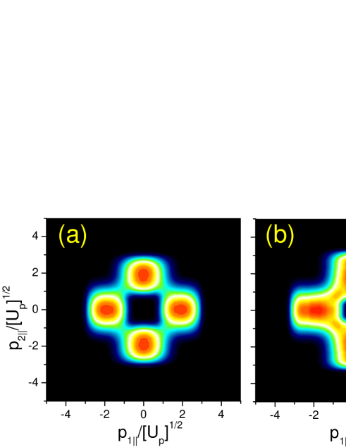
Figure 1: Electron momentum distributions for Helium ($E_{1g}=0.97$ a.u., $E_{2g}=2$ a.u. and $E_{2e}=0.5$ a.u.) in a linearly polarized, monochromatic field of frequency $\omega=0.057$ a.u.. In the picture, we considered all prefactors to be constant. Panels (a), (b) and (c) correspond to a driving-field intensity $I=2.16\times\mathrm{W/cm^{2}}$, $I=2.5\times\mathrm{W/cm^{2}}$ and $I=3\times\mathrm{W/cm^{2}}$, respectively. The contour plots have been normalized to the maximum probability in each panel.

As an overall feature, the distributions exhibit four peaks at $(p_{j||},p_{\nu||})=(\pm 2\sqrt{U_{p}},0),$ with $j,\nu=1,2$ and $j\neq\nu.$ These peaks agree well with the constraints discussed in the previous sections. This holds even if the driving-field intensity is just enough to excite the second electron and the only allowed momenta are $\pm 2\sqrt{U_{p}}$ [Fig. 1.(a)]. Physically, this means that the first electron will reach its parent ion most probably at a crossing of the driving field, reaching the detector with the most probable momenta of $\pm 2\sqrt{U_{p}},$ while the second electron will reach it with vanishing momentum.

The shapes of the distributions, however, differ considerably. Indeed, at the RESI threshold intensity [Fig. 1.(a)], one observes ring-shaped distributions. As the intensity increases, this distributions become more and more elongated along the $p_{n\parallel}$ axis [Fig. 1.(b)], until the maxima merge and cross-shaped distributions are observed [Fig. 1.(c)].

This change of shape may be understood by analyzing the momentum-space constraints. The widths of the distributions are determined by the tunnel ionization of the second electron from an excited state. This process has no classical counterpart and leads to distributions peaked at $p_{2\parallel}=0$ and which vanish at $p_{2\parallel}=\pm 2\sqrt{U_{p}}$, i.e., at the direct ATI cutoff. Increasing the intensity will only make the effective potential barrier smaller or wider, and thus affect the overall yield, but will not change such constraints.

The elongations in the distributions are determined by the rescattering of the first electron. This rescattering, in contrast, delimits a momentum region which is highly dependent on the driving-field intensity. Therefore, its width in momentum space will vary. Specifically, at the RESI threshold, there will be maxima in the distributions at $p_{1\parallel}=\pm 2\sqrt{U_{p}}$ due to the fact that the first electron rescatters most probably at a field crossing. However, as these are the only classically allowed momenta, the distributions will be fairly narrow around this value. With increasing driving-field intensity, the classically allowed region defined by Eq. (15) will become more and more extensive and this will cause the elongation.

Note that the electrons are indistinguishable so that the above-stated arguments hold upon the exchange $p_{1\parallel}\leftrightarrow p_{2\parallel}$. Hence, the horizontal and vertical axis in the parallel momentum plane will be equally affected.

III.2 Bound-state signatures

We will now investigate how the shape of the bound state to which the second electron is excited is imprinted on the electron momentum distributions. We will also employ different gauges and types of electron-electron interaction. Explicitly, we will assume that the second electron is either excited by a contact-type interaction $V_{12}^{(\delta)}(\mathbf{r}_{1}-\mathbf{r}_{2})=\delta(\mathbf{r}_{1}-\mathbf{r}_{2})$ or by a long-range, Coulomb type interaction $V_{12}^{(C)}(\mathbf{r}_{1}-\mathbf{r}_{2})=1/(\mathbf{r}_{1}-\mathbf{r}_{2})$. In the former case, $V_{12}^{(\delta)}(\mathbf{p}_{1}-\mathbf{k})=const.$, while in the latter case $V_{12}^{(C)}(\mathbf{p}_{1}-\mathbf{k})\sim 1/(\mathbf{p}_{1}-\mathbf{k})^{2}.$

In order to perform a direct comparison, we will take the same parameters as in Fig. 1, but incorporate the prefactors $V_{\mathbf{p}_{1}e\mathbf{,k}g}^{(1s\rightarrow 2s)}$ and $V_{\mathbf{p}_{2}e}^{(2s)}$, or $V_{\mathbf{p}_{1}e\mathbf{,k}g}^{(1s\rightarrow 2p)}$ and $V_{\mathbf{p}_{2}e}^{(2p)}$, corresponding to the $1s\rightarrow 2s$ or $1s\rightarrow 2p$ excitation with subsequent tunneling, respectively.

In Fig. 2, we consider the lowest intensity in the previous figure and the velocity gauge. If the electron is excited to the $2s$ state [Fig. 2.(a)], we observe four spots which are slightly elongated along the $p_{n\parallel}$ axis. Hence, in comparison to its constant prefactor counterpart, i.e.,Fig. 1.(a), there was a narrowing. This narrowing is caused by the interplay of two features in the prefactor $V_{\mathbf{p}_{2}e}^{(2s)}$. First, this prefactor exhibits two symmetric nodes, which, for vanishing transverse momentum are located at $p_{2\parallel}=\pm\sqrt{U_{p}}$. As the transverse momentum increases, these minima move towards vanishing parallel momenta. Second, $V_{\mathbf{p}_{2}e}^{(2s)}$ decreases very steeply with transverse momenta $\mathbf{p}_{2\perp}$. Hence, upon integration over this parameter, the main contributions will be caused by small values of $\mathbf{p}_{2\perp}$ and will vanish near $p_{2\parallel}=\pm\sqrt{U_{p}}$.

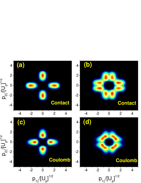
Figure 2: Velocity-gauge electron momentum distributions for Helium ($E_{1g}=0.97$ a.u., $E_{2g}=2$ a.u. and $E_{2e}=0.5$ a.u.) in a linearly polarized, monochromatic field of frequency $\omega=0.057$ a.u. and intensity $I=2.16\times\mathrm{W/cm^{2}}$. In panels (a) and (c), the first electron has been excited to $2s$, while in panels (b), and (d) it has been excited to $2p$. The interaction employed is indicated in the figure. The contour plots have been normalized to the maximum probability in each panel.

If, on the other hand, one assumes that the second electron is excited to $2p,$ there is both a broadening in the distributions and a splitting in their peaks. These features are depicted in Fig. 2.(b). The splitting occurs at the axis $p_{n\parallel}=0,n=1,2,$ and is caused by the fact that $V_{\mathbf{p}_{2}e}$ exhibits a very pronounced node at vanishing momenta, i.e., exactly where one expects $\mathrm{Im}[t]$ to be minimum and the yield to be maximum. This has been verified by a direct inspection of the radial dependence of Eq. (30), and omitting the $V_{\mathbf{p}_{2}e}$ prefactor in our computations. The latter procedure caused the additional minima to disappear (not shown). The broadening in the distributions as compared to the $1s\rightarrow 2s$ case is a consequence of the much slower decrease in $V_{\mathbf{p}_{2}e}^{(2p)}$ with increasing transverse momentum $p_{2\perp}$ and of the absence of the nodes at $p_{2\parallel}=\pm\sqrt{U_{p}}$. There are also additional nodes at the diagonal $p_{1||}=p_{2||}$ and at the anti-diagonal $p_{1||}=-p_{2||}$ of the $p_{1||}p_{2||}$ plane.

In this intensity regime, there seems to be little difference in the shapes of the distributions if the electron is excited to the $2s$ state, regardless of whether the first electron interacts with its parent ion through a contact or a Coulomb interaction [Figs. 2.(a) and (c), respectively]. This is possibly caused by the fact that the prefactor $V_{\mathbf{p}_{2}e}^{(2s)}$, due to its fast-decaying behavior, delimits a very narrow region in momentum space. This adds up to the very restrictive momentum constraints. In contrast, the effect of the Coulomb tail is much more critical if the electron is promoted to the $2p$ state. Indeed, for a Coulomb type interaction [Fig. 2.(d)], the splitting of the peaks at the axis $p_{n\parallel}=0$ remain, but the nodes at $p_{1||}=p_{2||}$ and $p_{1||}=-p_{2||}$ disappear as compared to its contact-interaction counterpart [Fig. 2.(b)]. This is caused by the fact that the former minima are a characteristic of the $V_{\mathbf{p}_{2}e}^{(2p)}$ prefactor, whereas the latter are mainly determined by momentum-space effects. The Coulomb interaction introduces a further momentum bias, and washes out the latter nodes.

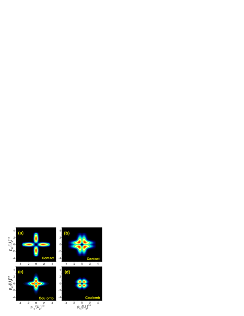
Figure 3: Velocity-gauge electron momentum distributions for the same parameters as in the previous figure, but driving-field intensity $I=3\times\mathrm{W/cm^{2}}$. In panels (a) and (c), the first electron has been excited to $2s$, while in panels (b), and (d) it has been excited to $2p$. The interaction employed is indicated in the figure. The contour plots have been normalized to the maximum probability in each panel.

We will now discuss what happens if the intensity of the driving field is such that $3.17U_{p}>E_{2g}-E_{2e}.$ These results are displayed in Fig. 3, for the highest intensity in Fig. 1. As expected, all distributions are much more elongated along the axis $p_{n\parallel}=0$, as compared to the low-intensity case. The imprint, however, of the different bound states to which the second electron is excited and from which it subsequently tunnels are the same as in the below-threshold regime. Indeed, we notice that there is a narrowing in the distributions for the $1s\rightarrow 2s$ case [Figs. 3.(a) and (c)], and a splitting in the peaks at the four axis in the $1s\rightarrow 2p$ case [Figs. 3.(b) and (d)]. This is not surprising, as the prefactors $V_{\mathbf{p}_{2}e}^{(2s)}$ and $V_{\mathbf{p}_{2}e}^{(2p)}$ exhibit the same functional dependencies as before.

The shapes of distributions, however, change much more critically in this intensity regime, with regard to the type of electron-electron interaction, than for the intensity used in Fig. 2. For all cases, the distributions computed using the Coulomb-type interaction (Figs. 3.(c) and  3.(d)) are much more localized in the low-momentum regions than those computed with a contact-type interaction (see Figs. 3.(a) and  3.(b)). This is expected, as $V_{12}(\mathbf{p}_{1}-\mathbf{k})$ favors low momenta for the former, while it is constant for the latter. Physically, this reflects the fact that rescattering of the first electron is now allowed to occur over an extensive region in momentum space. Hence, it does make a difference whether the second electron is excited by a long-range or zero-range interaction.

We will now perform an analysis of the electron-momentum distributions in the length gauge. In this case, the prefactor $V_{\mathbf{p}_{2}e}$ governing the tunneling of the second electron exhibits a singularity, and must be incorporated in the action. The modifications in the action read, for the $2s$ and $2p$ bound states,

$$-i\partial_{t}\ln V_{\mathbf{p}_{2}e}^{(2s)}=-i\frac{2E(t)\tilde{p}_{2}(t)_{\parallel}(\left[\tilde{p}_{2}(t)_{\parallel}\right]^{2}+\mathbf{p}_{2\perp}^{2}-6E_{2e})}{\chi_{+}(\mathbf{\tilde{p}}_{2}(t))\chi_{-}(\mathbf{\tilde{p}}_{2}(t))},$$ (40)

and

$$-i\partial_{t}\ln\tilde{V}_{\mathbf{p}_{2}e}^{(2p)}=i\frac{E(t)(\mathbf{p}_{2\perp}^{2}+2E_{2e}-3\left[\tilde{p}_{2}(t)_{\parallel}\right]^{2})}{\tilde{p}_{2}(t)_{\parallel}\left(\left[\tilde{p}_{2}(t)_{\parallel}\right]^{2}+\mathbf{p}_{2\perp}^{2}+2E_{2e}\right)},$$ (41)

respectively, with
$\chi_{\pm}(\mathbf{\tilde{p}}_{2}(t))=\left(\left[\tilde{p}_{2}(t)_{\parallel}\right]^{2}+\mathbf{p}_{2\perp}^{2}\pm 2E_{2e}\right)$ and $E(t)=-\partial_{t}A(t)$.

For each orbit, the tunneling time of the second electron will split into two values, as compared to the non-modified action. This has particularly important consequences as far as $\mathrm{Im}[t]$ is concerned, since it provides a rough measure of the width of the barrier through which the second electron tunnels. Physically, this means there will be one set of orbits for which the effective potential barrier will be widened, and another one for which it will be narrowed.

In Fig. 4, we present the contributions of each of the orbits resulting from this splitting for a final $2s$ state, for two different driving-field intensities. For simplicity, in order to single out the effect of the modified action, we took the rescattering prefactor $V_{\mathbf{p}_{1}e,\mathbf{k}g}$ to be constant.

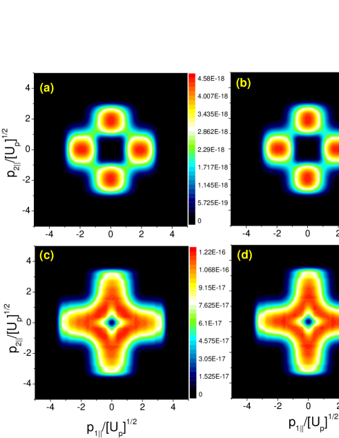
Figure 4: Length-gauge electron momentum distributions for Helium in a linearly polarized, monochromatic field. Throughout, we assumed $V_{\mathbf{p}_{1}e,\mathbf{k}g}=const.$, $V_{12}$ to be a contact-type interaction, and incorporated $V^{(2s)}_{\mathbf{p}_{2}e}$ in the action. Panels (a) and (c) correspond to the trajectories for which the barrier has been narrowed by the modifications in the action, while Panels (b) and (d) correspond to those for which it has been widened. The upper and lower panels correspond to driving field intensities $I=2.16\times 10^{14}\mathrm{W}/\mathrm{cm}^{2}$ and $I=3\times 10^{14}\mathrm{W}/\mathrm{cm}^{2}$, respectively. In order to perform a quantitative comparison, we are providing the explicit values for the NSDI yield.

In general, the distributions differ quantitatively in a factor between $1.5$ and $1.7$, depending on whether $\mathrm{Im}[t]$ decreased [Figs. 4(a) and (c)] or increased [Figs. 4(b) and (d)]. This shows that the splitting in this quantity is small, and therefore both contributions are comparable.

Furthermore, the distributions displayed in Fig. 4 are strikingly similar to those observed in Fig. 1 (see panels (a) and (c) therein), for which only constant prefactors have been considered. Indeed, the width of all distributions, along the axis, is determined by the direct ATI cutoff, i.e., $-2\sqrt{U_{p}}\leq p_{n\parallel}\leq 2\sqrt{U_{p}}$. At first sight, this is unexpected, as we are assuming that the second electron is tunneling from a $2s$ state. As previously discussed, the prefactor $V_{\mathbf{p}_{2}e}^{(2s)}$ exhibits a node in $p_{2\parallel}=\pm\sqrt{U_{p}}$, which leads to a narrowing of the distributions along the $p_{n\parallel}$ axis. An inspection of Eq. (24) also suggests that, were it not for its singularity, the length-gauge prefactor would be very similar to the velocity-gauge prefactor. This is a consequence of the fact that the second electron is leaving when the field $E(t)$ is near its maximum. For a monochromatic field, this implies that the vector potential $A(t)$ is practically vanishing.

One should note, however, that we are considering only the individual contributions from each of the orbits originating from the modification of the action. It is very likely that, in order to recover the structure determined by the prefactor $V^{(2s)}_{\mathbf{p}_{2}e}$, one must consider the coherent superposition of all the orbits originating from the splitting of $\mathrm{Im}[t]$ when computing the yield. Since these contributions are comparable, one expects the above-mentioned nodes to be recovered due to quantum-interference effects.

III.3 Comparison with experiments

We will now perform a direct comparison with the results in Ref. Eremina . In particular, in this reference, the distributions encountered have been modeled employing the electron-impact ionization physical mechanism and a modified ionization threshold for the second electron. Apart from that, however, in view of the driving-field intensities involved, one expects recollision-excitation tunneling to be present.

For that purpose, we will consider argon and the same laser-field parameters as in Ref. Eremina (c.f. Fig. 2 therein). We will assume, however, that, when the first electron recollides, it excites the second electron from the $3p$ state either to the $4s$ or to the $4p$ state. Thereby, we took the velocity gauge, and assumed that the first electron interacts with the ion by a Coulomb or contact interaction.

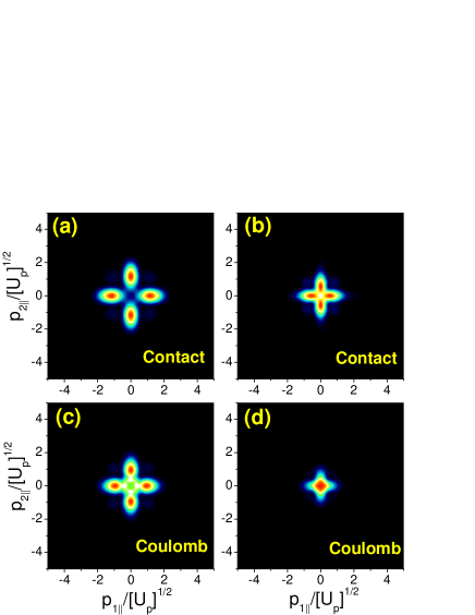
Figure 5: Velocity-gauge electron momentum distributions for Argon in a linearly polarized, monochromatic field of frequency $\omega=0.057$ a.u. The electron is excited from $3p$ to $4s$, i.e., $E_{1g}=0.58$ a.u., $E_{2g}=1.02$ a.u. and $E_{2e}=0.40$ a.u. in our calculations. The laser-field intensity in panels (a) and (c), and panels (b) and (d) is $I=9\times 10^{13}\mathrm{W}/\mathrm{cm}^{2}$ and $I=1.5\times 10^{14}\mathrm{W}/\mathrm{cm}^{2}$, respectively. The type of interaction $V_{12}$ taken is indicated in the figure. The contour plots have been normalized to the maximum probability in each panel. We have verified, however, that the highest yields on left-hand panels are between one and a half and two orders of magnitude smaller than those on the right-hand side.

The results for the $3p\rightarrow 4s$ excitation are presented in Fig. 5. An overall feature in the distributions are two main maxima along the $p_{n\parallel}$, $n=1,2$, axis. These features are mainly caused by the $V^{(4s)}_{\mathbf{p}_{2}e}$ prefactor for the tunnel ionization of the second electron, which decays very rapidly with increasing transverse momenta and exhibit nodes near $p_{2\parallel}=\pm 0.5\sqrt{U_{p}}$. In general, we have verified that this prefactor determines the shape of the electron-momentum distributions. Secondary maxima, around one order of magnitude smaller, occur due to the rescattering prefactor $V^{(3p\rightarrow 4s)}_{\mathbf{p}_{1}e,\mathbf{k}g}$. This prefactor exhibits an annular shape around $p_{1\parallel}=p_{2\parallel}=0$.

The existing experiments, however, do not lead to distributions concentrated along the axis of the $p_{1\parallel}p_{2\parallel}$ plane. The results for Helium in the previous section suggest that a $p$ state may lead to broader distributions. For that reason, we will assume that, instead, the second electron is excited to the $4p$ state.

Fig. 6 depicts the electron-momentum distributions for Argon under the assumption that the electron was excited from $3p$ to $4p$. All distributions in the figure exhibit four main maxima, which are broader than those in Fig. 5 and almost split at the axis $p_{n\parallel}=0$. These maxima are mainly determined by the prefactor $V^{(4p)}_{\mathbf{p}_{2}e}$, which has a node at the axis for low transverse momenta and nodes around $p_{2\parallel}=\pm\sqrt{U_{p}}$ across a wide transverse-momentum range. Apart from that, the prefactors $V^{(3p\rightarrow 4p)}_{\mathbf{p}_{1}e,\mathbf{k}g}$ decay more slowly with regard to the transverse momenta. This implies that, upon integration, a larger momentum region will be contributing to the NSDI yields. As in the previous case, this prefactor also leads to secondary maxima (see Figs. 6.(c) and (d) for concrete examples). In all cases, both in Figs. 5 and 6, a Coulomb type interaction mainly introduces a bias towards lower momenta.

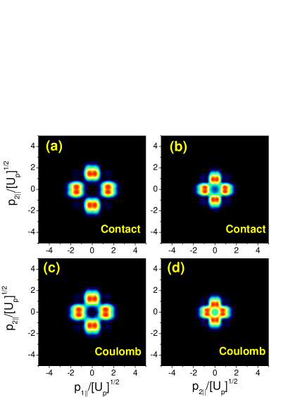
Figure 6: Velocity-gauge electron momentum distributions for Argon in a linearly polarized, monochromatic field of frequency $\omega=0.057$ a.u. The electron is excited from $3p$ to $4p$, i.e., $E_{1g}=0.58$ a.u., $E_{2g}=1.02$ a.u. and $E_{2e}=0.31$ a.u. in our calculations. The laser-field intensity in panels (a) and (c), and panels (b) and (d) is $I=9\times 10^{13}\mathrm{W}/\mathrm{cm}^{2}$ and $I=1.5\times 10^{14}\mathrm{W}/\mathrm{cm}^{2}$, respectively. The type of interaction $V_{12}$ taken is indicated in the figure. The contour plots have been normalized to the maximum probability in each panel. We have verified, however, that the highest yields on left-hand panels are between one and two orders of magnitude smaller than those on the right-hand side.

Despite the above-mentioned broadening, the electron-momentum distributions in Fig. 6 are still considerably narrower than those observed in Ref. Eremina . Within our framework, this constraint is imposed by the $V^{(4p)}_{\mathbf{p}_{2}e}$ prefactor. In fact, we have verified that, for large principal quantum number, this prefactor always exhibits nodes at lower absolute momenta than the ATI cutoff of $p_{2\parallel}=2\sqrt{U_{p}}$. In fact, if $V_{\mathbf{p}_{2}e}$ is taken to be constant, the distributions become considerably broader and a better agreement with the experiments is obtained. This is shown in Fig. 7, as ring-shaped distributions with four symmetric maxima at $p_{1\parallel}=p_{2\parallel}$ and $p_{1\parallel}=-p_{2\parallel}$. Such maxima are mainly determined by the $V^{(3p\rightarrow 4p)}_{\mathbf{p}_{1}e,\mathbf{k}g}$ prefactor. One should note, however, that this procedure is inconsistent from a theoretical perspective: Since the electron has been excited to the $4p$ state, it should subsequently tunnel from it. Hence, the pertaining prefactor must be taken.

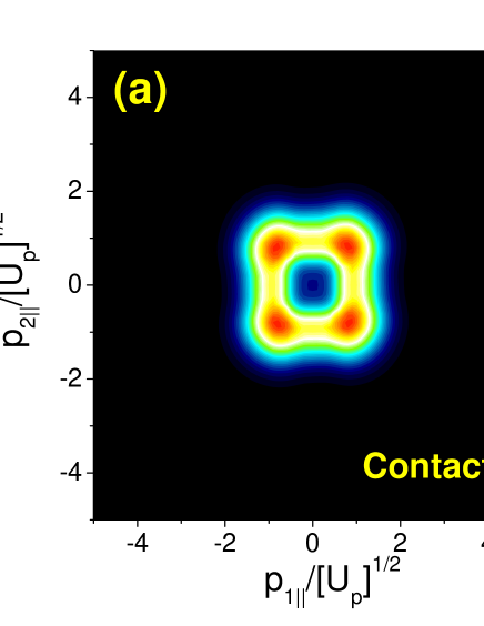
Figure 7: Velocity-gauge electron momentum distributions for Argon in a linearly polarized, monochromatic field of frequency $\omega=0.057$ a.u. and intensity $I=1.5\times 10^{14}\mathrm{W}/\mathrm{cm}^{2}$. The electron is excited from $3p$ to $4p$. We have taken the prefactor $V_{\mathbf{p}_{2},e}$ to be constant. The type of interaction $V_{12}$ is indicated in the figure. The contour plots have been normalized to the maximum probability in each panel.

IV Conclusions

Our analysis of the rescattering-excitation ionization (RESI) mechanism shows that the NSDI electron momentum distributions depend on the interplay between the relevant momentum-space regions, the type of interaction exciting the second electron, and the spatial dependence of the bound states involved. We will commence by discussing each of these issues separately.

The shapes of the electron momentum distributions, are determined by the interplay between two different behaviors, associated with the collision of the first electron and the tunneling of the second electron. The momentum region determined by the tunnel ionization of the second electron from an excited state will be always restricted by the direct ATI cutoff. The relevant momentum region will not change regardless of the driving-field intensity, as this will always be a classically forbidden process.

The first electron, on the other hand, rescatters inelastically with its parent ion, giving part of its kinetic energy upon return to excite the second electron. Hence, if its maximum return energy is larger than the energy difference $E_{2g}-E_{2e}$, rescattering has a classical counterpart. This implies that there will be a classically allowed region in momentum space. If, however, this energy is just enough to excite the second electron, the classical region will collapse. Hence, the extension of the relevant region in momentum space related to the rescattering of the first electron will depend on the driving-field intensity. Hence, the distributions become increasingly elongated as the intensity increases.

This also implies that one may define a threshold driving-field intensity for the RESI mechanism. This intensity is considerably lower than that necessary for the second ionization potential to be overcome by the second electron, i.e., for electron-impact ionization to occur.

Apart from that, we have observed that the bound states involved in the process leave very distinct fingerprints on the electron momentum distributions. This is particularly true for the bound state of the second electron, prior and subsequently to excitation. In fact, the widths of the distributions, their shapes and the number of maxima present will strongly depend on the principal and orbital quantum numbers of the bound states involved.

In contrast, the type of interaction $V_{12}$ by which the second electron is excited influences such distributions in a less drastic way. Indeed, a long-range, Coulomb interaction mainly introduces a bias towards lower momenta, as compared to a contact-type interaction.

A very important observation is that all distributions encountered in this work are equally spread over the four quadrants of the $p_{1\parallel}p_{2\parallel}$ plane. Under no circumstances have we found electron momentum distributions concentrated only on the second and fourth quadrant of this plane, as reported in the literature timelag ; NSDIalign ; Chen .

Within our framework, the above-stated symmetry can immediately be inferred from Eq. (III). Nonetheless, one could argue that our approach does not include the residual binding potential in the electron propagation in the continuum. Recent results, however, from a classical-trajectory computation in which the Coulomb potential has been incorporated, also revealed the same symmetry if only the RESI mechanism is singled out Agapi09 . This is a strong hint that our results are not an artifact of the strong-field approximation.

Hence, we suspect that, in the existing literature, the contributions from the RESI mechanism to nonsequential double ionization also equally occupy the four quadrants of the $p_{1\parallel}p_{2\parallel}$ plane. They may, however, be difficult to extract, as explained below.

In many situations addressed in the literature, the driving-field intensity is high enough for electron-impact ionization to occur. This means that this latter NSDI mechanism is also present, and fills the first and third quadrant of the $p_{1\parallel}p_{2\parallel}$ plane. Since, in many ab initio models, the different rescattering mechanisms are difficult to disentangle, the contributions from electron-impact ionization possibly obscure those from RESI in this region. In the second and fourth quadrant of the parallel momentum plane, the former contributions are absent and those from RESI can be more easily identified. In our approach, electron-impact ionization is absent from the start.

If the driving-field intensities are below the electron-impact ionization threshold, the second electron may no longer be provided with enough energy to overcome the second ionization potential. Consequently, RESI becomes more prominent and the distributions equally occupy the four quadrants of the parallel momentum plane. In fact, ring-shaped distributions centered around $p_{1\parallel}=p_{2\parallel}=0$ have been observed experimentally for this intensity region threshold ; Eremina .

Our results are far more localized near the $p_{n\parallel}=0$ axis than the experimental findings. This discrepancy may be due to the following reasons. First, for higher intensities employed in Ref. Eremina , collisional excitation may take place not only to the $4s$ or to the $4p$ state, but also to highly lying states, or to a coherent superposition of excited states. To take this into account may be needed in order to reproduce the experimental data.

Second, at the relevant driving-field intensities, one expects the excited states to be distorted by the field, and the propagation of the electron in the continuum near the core to be influenced by the residual ionic potential. This implies that a semi-analytical treatment beyond the strong-field approximation is necessary (see, e.g., corrections ; Denys for other phenomena and the electron-impact ionization case, respectively). Such a treatment is outside the scope of the present paper, and will be the topic of future work.

Acknowledgements: This work has been financed by the UK EPSRC (Grant no. EP/D07309X/1). We would also like to thank the UK EPSRC for the provision of a DTA studentship and of a summer studentship, and A. Emmanouilidou for providing her RESI results prior to publication. C.F.M.F. and T.S. are also grateful to the ICFO Barcelona for its kind hospitality.

V Appendix

In this appendix, we provide the general expressions for all prefactors employed in this paper. We will make no simplifying assumption on the initial states of the first and second electron, and on the excited state to which the second electron is promoted, apart from the fact that they are given by hydrogenic wavefunctions. In order to compute the prefactors, we will employ the expansion

$$e^{-i\mathbf{q}\cdot\mathbf{r}_{\alpha}} = 4\pi\sum_{l=0}^{\infty}\sum_{m=-l}^{l}(-i)^{l}j_{l}(qr_{\alpha})$$ (42)

$$Y_{l}^{m}(\theta_{q_{\alpha}},\varphi_{q_{\alpha}})\left[Y_{l^{\prime}}^{m^{\prime}}(\theta_{\alpha},\varphi_{\alpha})\right]^{\ast},$$

where $\mathbf{q}$ denotes a generic momentum, $\mathbf{r}_{\alpha}$ the coordinate of the ${\alpha}^{th}$ electron, and $j_{l}(\cdot)$ the spherical Bessel functions of the first kind. This expression will be both used in the derivation of $V_{\mathbf{p}_{2}e}$ and $V_{\mathbf{p}_{1}e\mathbf{,k}g},$ together with the orthogonality relation

$$\int\left[Y_{l^{\prime}}^{m^{\prime}}(\theta_{\alpha},\varphi_{\alpha})\right]^{\ast}Y_{l}^{m}(\theta_{\alpha},\varphi_{\alpha})d\Omega=\delta_{ll^{\prime}}\delta_{mm^{\prime}},$$ (43)

where $\Omega$ denotes the solid angle.

For the former prefactor, Eq. (5) reduces to

$$V_{\mathbf{p}_{2}e} \sim \int\int\exp[-i(\mathbf{\tilde{p}}_{2}(t)\cdot\mathbf{r}_{2})]R_{nl}(r_{2})Y_{l}^{m}(\theta_{2},\varphi_{2})r_{2}dr_{2}d\Omega$$ (44)

$$= 4\pi(-i)^{l}Y_{l}^{m}(\theta_{\tilde{p}_{2}},\varphi_{\tilde{p}_{2}})\mathcal{I}_{1},$$

with

$$\mathcal{I}_{1}=\int_{0}^{\infty}r_{2}R_{nl}(r_{2})j_{l}(\tilde{p}_{2}(t)r_{2})dr_{2}.$$ (45)

Similarly, Eq. (6) reads

$$V_{\mathbf{p}_{1}e\mathbf{,k}g}\sim V_{12}(\mathbf{p}_{1}-\mathbf{k})\mathcal{I}_{2},$$ (46)

with

$$\mathcal{I}_{2} = \int d^{3}r_{2}e^{i(\mathbf{k-p}_{1})\cdot\mathbf{r}_{2}}R_{n_{e}l_{e}}(r_{2})\left[Y_{l_{e}}^{m_{e}}(\theta_{2},\varphi_{2})\right]^{\ast}$$ (47)

$$R_{n_{g}l_{g}}(r_{2})Y_{l_{g}}^{m_{g}}(\theta_{2},\varphi_{2}),$$

where the indices $g$ and $e$ in the principal, orbital and magnetic quantum numbers refer to the ground and excited states, respectively.

We will now compute the radial integrals $\mathcal{I}_{1}$ and $\mathcal{I}_{2}$ explicitly. For that purpose, let us consider a generic Hydrogenic radial wavefunction

$$R_{nl}(r) = C_{nl}r^{l}\exp[-\sqrt{2E_{n}}r]$$ (48)

$$\times\sum_{\nu=0}^{n-l-1}\frac{2^{\nu}(-1)^{\nu+1}(\sqrt{2E_{n}})^{\nu}}{\nu!(n-l-1-\nu)!(2l+1+\nu)!},$$

with

$$C_{nl}=-\left\{\frac{(2\sqrt{2E_{n}})^{3+2l}(n-l-1)!}{2n\left[(n+l)!\right]^{3}}\right\}^{1/2}\left[(n+l)!\right]^{2}.$$ (49)

In the above-stated equations, $E_{n}$ denotes the energy of the bound state to be studied, i.e., $n=2g$ or $n=2e$ for the ground or excited states of the second electron, respectively. Since we are performing a qualitative analysis, we will concentrate mostly on the functional form of $R_{nl}(r).$ The integral $\mathcal{I}_{1}$ present in the prefactor $V_{\mathbf{p}_{2}e}$ can then be written as

$$\mathcal{I}_{1} \varpropto \sum_{\nu=0}^{n-l-1}\frac{(-1)^{\nu+1}2^{\nu-1-l}(\sqrt{2E_{n}})^{-2-l}}{\nu!(n-l-1-\nu)!(2l+1+\nu)!}\frac{\Gamma\left[2+\nu+2l\right]}{\Gamma\left[3/2+l\right]}$$ (50)

$$\times_{2}F_{1}(1+l+\frac{\nu}{2},\frac{3+\nu}{2}+l,\frac{3}{2}+l,-\frac{\left[\tilde{p}_{2}(t)\right]^{2}}{2E_{e}}).$$

The integral $\mathcal{I}_{2}$ in $V_{\mathbf{p}_{1}e\mathbf{,k}g}$ is slightly more involved. It may be explicitly written as

$$\mathcal{I}_{2}=4\pi\sum_{l=0}^{\infty}\sum_{m=-l}^{l}(-i)^{l}Y_{l}^{m}(\theta_{q_{\alpha}},\varphi_{q_{\alpha}})\mathcal{I}_{2R}\mathcal{I}_{2\Omega},$$ (51)

where

$$\mathcal{I}_{2R}=\int_{0}^{\infty}r_{2}^{2}R_{n_{g}l_{g}}(r_{2})R_{n_{e}l_{e}}(r_{2})j_{l}(\kappa r_{2})dr_{2}$$ (52)

and

$$\mathcal{I}_{2\Omega}=\int Y_{l}^{m}(\theta_{2},\varphi_{2})\left[Y_{l_{e}}^{m_{e}}(\theta_{2},\varphi_{2})\right]^{\ast}Y_{l_{g}}^{m_{g}}(\theta_{2},\varphi_{2})d\Omega$$ (53)

give the radial and angular dependencies of such prefactors, respectively. The explicit expression for $\mathcal{I}_{2}$ is then

$$\mathcal{I}_{2} = 4\pi\sum_{l=|l_{g}-l_{e}|}^{l_{g}+l_{e}}\sum_{m=-l}^{l}(-i)^{l}(-1)^{m_{e}}Y_{l}^{m}(\theta_{\kappa},\varphi_{\kappa})\sqrt{\frac{\left(2l_{g}+1\right)\left(2l_{e}+1\right)}{4\pi\left(2l+1\right)}}$$ (54)

$$\times\left\langle l_{g},l_{e},0,0\right.\left|l,0\right\rangle\left\langle l_{g},l_{e},m_{g},-m_{e}\right.\left|l,0\right\rangle\mathcal{I}_{2R}.$$

The radial integral $\mathcal{I}_{2R}$ is proportional to

$$\mathcal{I}_{2R} \propto \sum_{\nu_{g}=0}^{n_{g}-l_{g}-1}\sum_{\nu_{e}=0}^{n_{e}-l_{e}-1}\frac{(-1)^{\nu_{e}+\nu_{g}+1}2^{\nu_{e}+\nu_{g}-1-l}(\sqrt{2E_{2g}})^{\nu_{g}}(\sqrt{2E_{2e}})^{\nu_{e}}\left[\zeta(E_{2g},E_{2e})\right]^{-3-\nu_{e}-\nu_{g}-l_{e}-l_{g}}}{\nu_{e}!\nu_{g}!(n_{e}-l_{e}-1-\nu_{e})!(n_{g}-l_{g}-1-\nu_{g})!(2l_{e}+1+\nu_{e})!(2l_{g}+1+\nu_{g})!}$$ (55)

$$\frac{\Gamma\left[2+\lambda\right]}{\Gamma\left[3/2+l\right]}\left(\frac{\kappa^{2}}{\zeta^{2}(E_{2g},E_{2e})}\right)^{l/2}_{2}F_{1}(\frac{3+\lambda}{2},\frac{4+\lambda}{2},\frac{3}{2}+l,-\frac{\kappa^{2}}{\zeta^{2}(E_{2g},E_{2e})}),$$

where $\lambda=\nu_{e}+\nu_{g}+l_{e}+l_{g}+l$ and $\zeta(E_{2g},E_{2e})$ is defined according to Eq. (23). Note that the terms in Eq. (54) are only non-vanishing if $m=m_{g}-m_{e}$ and $l_{1}+l_{2}-l$ is even.

In the present work, apart from the case in which only $s$ states are involved and the angular integrals are constant, one may identify the following cases. First, the second electron may be initially in a $p$ state and be excited to an $s$ state. In this case, $l=l_{g}=1$ and $l_{e}=0$. Second, if the electron is initially in an $s$ state and is excited to a $p$ state, then $l=l_{e}=1$ and $l_{g}=0$. Finally, if the second electron suffers a transition from a $p$ state to another $p$ state, in principle $l=0,1,2$. Due to the constraints upon $l$ for the Clebsch-Gordan coefficients, however, only the terms with $l=0,2$ will survive. Apart from that, the constraint upon $m$ will impose further restrictions for $m_{e}$ and $m_{g}$. The above-stated expressions, however, are applicable to generic hydrogenic states.

References

- (1) For reviews on this subject see, e.g., R. Dörner, Th. Weber, M. Weckenbrock, A. Staudte, M. Hattas, H.Schmidt-Bocking, R. Moshammer, J. Ullrich: Adv. At., Mol., Opt. Phys. 48, 1 (2002); J. Ullrich, R. Moshammer, A. Dorn, R. Dörner, L. Ph. H. Schmidt, and H. Schmidt-Böcking, Rep. Prog. Phys. 66, 1463 (2003).
- (2) A. L’Huillier, L. A. Lompr, G. Mainfray, and C. Manus, Phys. Rev. A 27, 2503 (1983); B. Walker, B. Sheehy, L. F. DiMauro, P. Agostini, K. J. Schafer, and K. C. Kulander, Phys. Rev. Lett. 73, 1227 (1994).
- (3) See, e.g., Th. Weber, M. Weckenbrock, A. Staudte, L. Spielberger, O. Jagutzki, V. Mergel, F. Afaneh, G. Urbasch, M. Vollmer, H. Giessen, and R. Dörner, Phys. Rev. Lett. 84, 443 (2000); R. Moshammer, B. Feuerstein, W. Schmitt, A. Dorn, C. D. Schröter, J. Ullrich, H. Rottke, C. Trump, M. Wittmann, G. Korn, K. Hoffmann, and W. Sandner, Phys. Rev. Lett. 84, 447 (2000).
- (4) P. B. Corkum, Phys. Rev. Lett. 71, 1994 (1993).
- (5) See, e.g., A. Becker and F. H. M. Faisal, Phys. Rev. Lett. 84, 3546 (2000); A. Becker and F. H. M. Faisal, Phys. Rev. Lett. 89, 193003 (2002); S. V. Popruzhenko and S. P. Goreslavskii, J. Phys. B 34, L239 (2001); S. P. Goreslavski and S. V. Popruzhenko, Opt. Express 8, 395 (2001); S. P. Goreslavskii, S. V. Popruzhenko, R. Kopold, and W. Becker, Phys. Rev. A 64, 053402 (2001).
- (6) C. Figueira de Morisson Faria, H. Schomerus, X. Liu, and W. Becker, Phys. Rev. A 69, 043405 (2004).
- (7) C. Figueira de Morisson Faria, and M. Lewenstein, J. Phys. B 38, 3251 (2005).
- (8) M. Lein, E. K. U. Gross, and V. Engel, Phys. Rev. Lett. 85, 4707 (2000); J. Phys. B 33, 433 (2000); J. S. Parker, B. J. S. Doherty, K. T. Taylor, K. D. Schulz, C. I. Blaga and L. F. DiMauro, Phys. Rev. Lett. 96, 133001 (2006).
- (9) X. Liu and C. Figueira de Morisson Faria, Phys. Rev. Lett. 92, 133006 (2004); C. Figueira de Morisson Faria, X. Liu, A. Sanpera and M. Lewenstein, Phys. Rev. A 70, 043406 (2004).
- (10) J. S. Prauzner-Bechcicki, K. Sacha, B. Eckhardt, and J. Zakrzewski, Phys. Rev. A 78, 013419 (2008).
- (11) A. Staudte, C. Ruiz, M. Schöffler, D. Zeidler, Th. Weber, M. Meckel, D.M. Villeneuve, P.B. Corkum, A. Becker and R. Dörner, Phys. Rev. Lett. 99, 263002 (2007); A. Rudenko, V. L. B. de Jesus, Th. Ergler, K. Zrost, C. D. Schröter, R. Moshammer and J. Ullrich, Phys. Rev. Lett. 99, 263003 (2007).
- (12) A. Emmanouilidou, Phys Rev A 78, 023411 (2008); D. F. Ye, X. Liu, and J. Liu, Phys. Rev. Lett. 101, 233003 (2008).
- (13) Denys I. Bondar, Wing-Ki Liu, and Misha Yu. Ivanov, Phys. Rev. A 79, 023417 (2009).
- (14) E. Eremina, X. Liu, H. Rottke, W. Sandner, A. Dreischuch, F. Lindner, F. Grasbon, G.G. Paulus, H. Walther, R. Moshammer, B. Feuerstein, and J. Ullrich, J. Phys. B. 36, 3269 (2003).
- (15) E. Eremina, X. Liu, H. Rottke, W. Sandner, M. G. Schätzel, A. Dreischuh, G. G. Paulus, H. Walther, R. Moshammer, and J. Ullrich, Phys. Rev. Lett. 92, 173001 (2004); Yunquan Liu, S. Tschuch, A. Rudenko, M. Dürr, M. Siegel, U. Morgner, R. Moshammer, and J. Ullrich, Phys. Rev. Lett. 101, 053001 (2008).
- (16) S. L. Haan, L. Breen, A. Karim and J. H. Eberly, Phys. Rev. Lett. 97, 103008 (2006).
- (17) See, e.g., V. L. B. de Jesus, B. Feuerstein, K. Zrost, D. Fischer, A. Rudenko, F. Afaneh, C.D. Schröter, R. Moshammer, and J. Ullrich, J. Phys. B 37, L161 (2004).
- (18) R. Kopold, W. Becker, H. Rottke and W. Sandner, Phys. Rev. Lett. 85, 3871 (2000).
- (19) J. S. Prauzner-Bechcicki, K. Sacha, B. Eckhardt, and J. Zakrzewski, Phys. Rev. A 71, 033407 (2005).
- (20) Y. Li, J. Chen, S. P. Yang, and J. Liu, Phys. Rev. A 76, 023401 (2007); J. Liu, D. F. Ye, J. Chen and X. Liu, Phys. Rev. Lett. 99, 013003 (2007); D. F. Ye, J. Chen, and J. Liu, Phys. Rev A 77, 013403 (2008).
- (21) D. Zeidler, A. Staudte, A. B. Bardon, D. M. Villeneuve, R. Dörner, and P. B. Corkum, Phys. Rev. Lett. 95, 203003 (2005); D. F. Ye, J. Chen, and J. Liu, Phys. Rev. A 77, 013403 (2008).
- (22) S. Baier, C. Ruiz, L. Plaja and A. Becker, Phys. Rev. A 74, 033405 (2006); S. Baier, C. Ruiz, L. Plaja, and A. Becker, Laser Phys. 17, 358 (2007); S. Baier, A. Becker and L. Plaja, Phys. Rev. A 78, 013409 (2008).
- (23) C. Figueira de Morisson Faria, T. Shaaran, X. Liu and W. Yang, Phys. Rev. A 78, 043407 (2008).
- (24) R. Panfili, J.H. Eberly, and S. L. Haan, Opt. Express 8, 431 (2001); R. Panfili, S. L. Haan, and J. H. Eberly, Phys. Rev. Lett. 89, 113001 (2002); P. J. Ho, R. Panfili, S. L. Haan and J. H. Eberly, Phys. Rev. Lett. 94, 093002 (2005).
- (25) A. Emmanouilidou and A. Staudte, Phys. Rev. A 80, 053415 (2009).
- (26) T. Shaaran and C. Figueira de Morisson Faria, arXiv:0906. 4229 (J. Mod. Opt., in press)
- (27) P. Salières, B. Carré, L. Le Déroff, F. Grasbon, G. G. Paulus, H. Walther, R. Kopold, W. Becker, D. B. Milošević, A. Sanpera, and M. Lewenstein, Science 292, 902 (2001).
- (28) B. Feuerstein, R. Moshammer, D. Fischer, A. Dorn, C. D. Schröter, J. Deipenwisch, J. R. Crespo Lopez-Urrutia, C. Höhr, P. Neumayer, J. Ullrich, H. Rottke, C. Trump, M. Wittman, G. Korn and W. Sandner, Phys. Rev. Lett. 87, 043003 (2001).
- (29) C. Figueira de Morisson Faria, H. Schomerus, and W. Becker, Phys. Rev. A 66, 043413 (2002).
- (30) O. Smirnova, M. Spanner and M. Ivanov, J. Phys. B 39, S323 (2006); O. Smirnova, A. S. Mouritzen, S. Patchkovskii and M. Ivanov, J. Phys. B 40 (2007); O. Smirnova, M. Spanner and M. Ivanov, Phys. Rev. A 77, 033407 (2008), S. V. Popruzhenko and D. Bauer, J. Mod. Opt. 55, 2573 (2008).