Abstract

We review the geometrical properties of vacuum spacetimes in (2+1)-gravity with vanishing cosmological constant. We explain how these spacetimes are characterised as quotients of their universal cover by holonomies. We explain how this description can be used to clarify the geometrical interpretation of the fundamental physical variables of the theory, holonomies and Wilson loops. In particular, we discuss the role of Wilson loop observables as the generators of the two fundamental transformations that change the geometry of (2+1)-spacetimes, grafting and earthquake. We explain how these variables can be determined from realistic measurements by an observer in the spacetime.

1 Introduction

Gravity in (2+1) dimensions serves as a toy model that allows one to investigate conceptual questions of (quantum) gravity in a mathematically tractable theory. As many questions related to time, light and causality cannot be addressed in a Euclidean framework, (2+1)-spacetimes of Lorentzian signature are particularly relevant in this context. These spacetimes have a rich geometry, for an overview see [1, 2], and realistic physical features such as initial (big bang) singularities and cosmological time functions.

In order to obtain interesting physics from these models, one needs to relate the variables which are used in the parametrisation of the phase space and in the quantisation of the theory to the geometry of the associated spacetime. This has proven challenging even in the classical theory. It is not obvious what is the geometrical interpretation of the fundamental diffeomorphism invariant observables (Wilson loops) and the associated phase space transformations they generate via the Poisson bracket. It is also not apparent how these variables could be determined through measurements performed by an observer in the spacetime.

In this paper, we summarise the results of [3, 4, 5] which provide an answer to these questions. In Section 2 we review Lorentzian (2+1)-spacetimes without matter and cosmological constant. We discuss their geometrical properties and their description as quotients of their universal cover. Section 3 introduces the two fundamental transformations that change the geometry of these spacetimes, grafting and earthquake along closed spacelike geodesics [6]. In Section 4 we explain how these two geometry changing transformations are generated via the Poisson bracket by the two fundamental Wilson loop observables associated to the geodesic. This provides a physical interpretation of Wilson loop observables. In Section 5 we discuss how the fundamental variables of the theory (holonomies and Wilson loops) can be determined from measurements by observers in the spacetime.

2 Vacuum spacetimes in (2+1)-gravity

2.1 Gravity in (2+1)-dimensions

As the Ricci curvature on a three-dimensional manifold determines its sectional curvature, vacuum solutions of the three-dimensional Einstein equations without cosmological constant are flat. The theory has no local gravitational degrees of freedom, and its solutions are locally isometric to three-dimensional Minkowski space $\mathbb{M}^{3}$. The solutions considered in this paper are obtained as quotients of regions in Minkowski space $\mathbb{M}^{3}$ by discrete subgroups of its isometry group. This subgroup encodes the global physical degrees of freedom of the theory which arise from the non-trivial topology of the spacetimes.

The group of orientation and time orientation preserving isometries of Minkowski space is the three-dimensional Poincaré group $P_{3}=SO^{+}(2,1)\ltimes\mathbb{R}^{3}$, which is the semidirect product of the proper orthochronous Lorentz group $SO^{+}(2,1)$ in three dimensions with the translation group $\mathbb{R}^{3}$. In the following, we parametrise elements of $P_{3}$ as $(u,{\mbox{\boldmath$a$}})$ with $u\in SO^{+}(2,1)$ and ${\mbox{\boldmath$a$}}\in\mathbb{R}^{3}$. The group multiplication law of $P_{3}$ then takes the form

$$(u_{1},{\mbox{\boldmath$a$}}_{1})\cdot(u_{2},{\mbox{\boldmath$a$}}_{2})=(u_{1}u_{2},{\mbox{\boldmath$a$}}_{1}+u_{1}{\mbox{\boldmath$a$}}_{2}).$$ (2.1)

We denote by $\exp:\mathfrak{so}(2,1)\rightarrow SO^{+}(2,1)$ the exponential map and introduce a basis $\{J_{a}\}_{a=0,1,2}$ of $\mathfrak{so}(2,1)$ in which the Lie bracket is given by $[J_{a},J_{b}]=\epsilon_{abc}J^{c}$. Here and in the following indices are raised and lowered with the Minkowski metric $\eta=\text{diag}(-1,1,1)$ and $\epsilon$ is the totally antisymmetric tensor in three indices with $\epsilon_{012}=1$.

2.2 Classification and geometry of (2+1)-spacetimes without matter

Under certain additional assumptions, the absence of local gravitational degrees of freedom allows one to classify the solutions of the (2+1)-dimensional vacuum Einstein equations. Such a classification has been achieved for maximally globally hyperbolic (MGH) flat (2+1)-spacetimes $M$ with geodesically complete Cauchy surfaces [6, 7]. The condition of global hyperbolicity is imposed to exclude spacetimes with bad causality properties. It ensures the absence of closed, timelike curves and the existence of a Cauchy surface $S$, a spacelike surface that every inextensible causal curve intersects exactly once. It also implies that $M$ is of topology $M\approx\mathbb{R}\times S$ and $\pi_{1}(M)\cong\pi_{1}(S)$. The maximality is a technical condition that avoids over-counting spacetimes, and the completeness condition excludes Cauchy surfaces with singularities.

It is shown in [8] that the universal cover $\tilde{M}$ of a MGH flat (2+1)-spacetime $M$ with a complete Cauchy surface can be identified with a domain of dependence in Minkowski space, i. e. the future of a set of points in $\mathbb{M}^{3}$. One distinguishes the following four cases:

Case 1: $\pi_{1}(M)=\{1\}$.

In this case $\tilde{M}=M$ is either the entire Minkowski space $\mathbb{M}^{3}$ or the future of a lightlike plane $P$ or the intersection of the future of a lightlike plane $P$ with the past of a lightlike plane $Q$ parallel to $P$.

Case 2: $\pi_{1}(M)=\mathbb{Z}$ (Cylinder universe).

In this case, the Cauchy surface has the topology of a cylinder, and the domains are the same as in case 1. The elements of $\pi_{1}(M)$ act by spacelike translations.

Case 3: $\pi_{1}(M)=\mathbb{Z}\oplus\mathbb{Z}$ (Torus universe).

In this case, the domain is either Minkowski space $\tilde{M}=\mathbb{M}^{3}$, and both generators of $\pi_{1}(M)$ act by spacelike translations as shown in Figure 1 a) or $\tilde{M}$ is the future of a spacelike line as shown in Figure 1 b). In that case, one of the generators acts by spatial translations in the direction of the geodesic’s tangent vector, while the other is a boost with this tangent vector as its axis.

Case 4: $\pi_{1}(M)\neq\{1\},\mathbb{Z},\mathbb{Z}\oplus\mathbb{Z}$ (Higher genus case).

In this case, $\tilde{M}$ is the future of set of points different from a geodesic line. The Lorentzian part of the holonomy $h:\pi_{1}(M)\rightarrow SO^{+}(2,1)$ defines a faithful and discrete representation of $\pi_{1}(M)$.

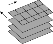
a) b)

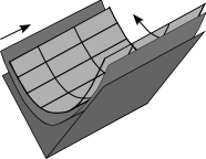
Figure 1: Universal cover for the torus universe. Case a): Static torus universe; $\tilde{M}=\mathbb{M}^{3}$. Case b:) Evolving torus universe; the universal cover $\tilde{M}$ is the future of a spacelike geodesic in $\mathbb{M}^{3}$. The grids and arrows indicate the action of $\pi_{1}(M)$ on $\tilde{M}$.

As case 1 and 2 have too few degrees of freedom and case 3 has been investigated extensively (for an overview see [1], for a discussion of observers and geometry [9]), we focus on case 4 in the following. Moreover, we restrict attention to the simplest case, namely to spacetimes which have a compact, orientable Cauchy surface $S$ of genus $g\geq 2$.

In this case, the universal cover $\tilde{M}$ is either the future of a point ${\mbox{\boldmath$p$}}\in\mathbb{M}^{3}$ or of a graph $G\subset\mathbb{M}^{3}$ [2, 6, 8]. Both, $M$ and $\tilde{M}$, are future complete and have an initial singularity. Moreover, it is shown in [2, 6, 10] that $M$ and $\tilde{M}$ are equipped with a cosmological time function, which gives the geodesic distance of points in $M,\tilde{M}$ from the initial singularity, and that they are foliated by surfaces $M_{T},\tilde{M}_{T}$ of constant cosmological time.

The fundamental group $\pi_{1}(M)$ acts on $\tilde{M}$ freely and properly discontinuously in such a way that each constant cosmological time surface $\tilde{M}_{T}$ is preserved. This group action is given by the holonomies, a group homomorphism $h:\pi_{1}(M)\rightarrow P_{3}$ into the isometry group of Minkowski space. The Lorentzian components $v_{\lambda}$ of the holonomies $h(\lambda)=(v_{\lambda},{\mbox{\boldmath$a$}}_{\lambda})$, $\lambda\in\pi_{1}(M)$, define a cocompact Fuchsian group of genus $g$. This is a discrete subgroup $\Gamma\subset SO^{+}(2,1)$ of the three-dimensional Lorentz group with $2g$ generators and a single defining relation, which is isomorphic to $\pi_{1}(M)$

$$\Gamma=\langle v_{a_{1}},v_{b_{1}},...,v_{a_{1}},v_{b_{1}}\;|\;[v_{B_{g}},v_{A_{g}}]\cdots[v_{B_{1}},v_{A_{1}}]=1\rangle\qquad[v_{b_{i}},v_{a_{i}}]=v_{b_{i}}v_{a_{i}}v_{b_{i}}^{-1}v_{a_{i}}^{-1}.$$ (2.2)

The spacetime $M$ is obtained as the quotient of $\tilde{M}$ by this group action, i. e. by identifying on each surface $\tilde{M}_{T}$ the points that are mapped into each other by the holonomies

$$M=\bigcup_{T\in\mathbb{R}^{+}}M_{T}=\bigcup_{T\in\mathbb{R}^{+}}\tilde{M}_{T}/\pi_{1}(M)_{h}.$$ (2.3)

The simplest example are the conformally static spacetimes for which the universal cover is a lightcone, i.e. the future of a point ${\mbox{\boldmath$p$}}\in\mathbb{M}^{3}$. In this case, the constant cosmological time surfaces are hyperboloids $\tilde{M}_{T}=T\cdot{\mathbb{H}^{2}}$ as depicted in Figure 2 a). As the action of $\pi_{1}(M)$ on $\tilde{M}$ preserves these hyperboloids, its translational component is trivial, i. e. given by conjugation

$$h(\lambda)=(1,-{\mbox{\boldmath$p$}})\cdot(v_{\lambda},0)\cdot(1,{\mbox{\boldmath$p$}})\qquad\forall\lambda\in\pi_{1}(M).$$ (2.4)

The action of $\pi_{1}(M)$ on the surfaces $\tilde{M}_{T}$ coincides with the canonical action of the associated Fuchsian group $\Gamma$ on two-dimensional hyperbolic space ${\mathbb{H}^{2}}$. This group action induces a tessellation of each constant cosmological time surface by geodesic arc $4g$-gons which are mapped into each other by the elements of $\Gamma$. The elements of $\Gamma$ identify the sides of these geodesic arc $4g$-gons pairwise as indicated in Figure 2 b).

The constant cosmological time surfaces $M_{T}$ are obtained by identifying the points on the hyperboloids $\tilde{M}_{T}$ which are related by this action of $\Gamma$. This amounts to gluing the sides of each polygon pairwise as shown in Figure 2 b). Each constant cosmological time surface $M_{T}$ is thus a copy of the same Riemann surface as in Figure 2 c), rescaled by the cosmological time $M_{T}=T\cdot\Sigma_{\Gamma}=T\cdot{\mathbb{H}^{2}}/\Gamma$ and thus equipped with a metric of constant curvature $-1/T^{2}$. As the geometry of the constant cosmological time surfaces $M_{T}$ evolves with $T$ only by a rescaling, these spacetimes are called conformally static.

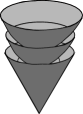
a)​​​​ ​​​​ ​​​​ b) c)

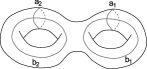
Figure 2: a) Foliation of the lightcone by hyperboloids. b) Identification of points in $\tilde{M}_{T}\cong{\mathbb{H}^{2}}$ for a genus $g=2$-surface. c) Resulting genus $g=2$ Riemann surface.

2.3 Phase space

It is shown in [6], see also [7], that flat maximally globally hyperbolic (2+1)-spacetimes of genus $g\geq 2$ and their universal covers are characterised uniquely by the holonomies $h:\pi_{1}(M)\rightarrow P_{3}$. Two spacetimes are isometric if and only if the associated holonomies are related by global conjugation with a constant element of $P_{3}$. Moreover, each group homomorphism $h:\pi_{1}(M)\rightarrow P_{3}$ whose Lorentzian component defines a cocompact Fuchsian group of genus $g$ gives rise to such a spacetime. This implies that the physical phase space of the theory, the space of solutions of the (2+1)-Einstein equations modulo diffeomorphisms, coincides with the cotangent bundle $T^{*}\tau_{g}$ of Teichmüller space $\tau_{g}$ and is given by

$$\mathcal{P}=\text{Hom}_{0}(\pi_{1}(S),P_{3})/P_{3}=T^{*}\tau_{g},$$ (2.5)

where the index $0$ indicates the restriction on the Lorentzian component of the holonomy. The phase space is equipped with a canonical symplectic structure, the Goldman bracket [11].

The physical (diffeomorphism invariant) observables of the theory are functions on $\mathcal{P}$ or, equivalently, functions of the holonomies $h(\lambda)$, $\lambda\in\pi_{1}(M)$, which are invariant under simultaneous conjugation with $P_{3}$. A complete set of such observables is given by the Wilson loops. In the case at hand, there are two canonical Wilson loop observables associated to each element $\lambda\in\pi_{1}(M)$. The first, in the following referred to as mass and denoted $m_{\lambda}$, depends only on the Lorentzian component of the associated holonomy, while the second, the spin $s_{\lambda}$, involves both the Lorentzian and the translational component

$$m_{\lambda}=\sqrt{{\mbox{\boldmath$p$}}_{\lambda}^{2}}\qquad s_{\lambda}=\hat{\mbox{\boldmath$p$}}_{\lambda}\cdot{\mbox{\boldmath$a$}}_{\lambda}\qquad\text{where}\qquad h(\lambda)=(\exp(p^{a}_{\lambda}J_{a}),{\mbox{\boldmath$a$}}_{\lambda}),\;\hat{\mbox{\boldmath$p$}}_{\lambda}={\mbox{\boldmath$p$}}_{\lambda}/m_{\lambda}$$ (2.6)

These Wilson loop observables are closely related to the two Casimir operators of the three-dimensional Poincaré algebra and play a fundamental role in the quantisation of the theory.

3 Construction of spacetimes via earthquake and grafting

Given a conformally static spacetime $M$ and a closed, simple geodesic $\lambda$ on a constant cosmological time surface $M_{T}$, there are two canonical ways of changing the geometry of $M$ [12, 13]: grafting and earthquake. The ingredients in the construction are a cocompact Fuchsian group $\Gamma$, given by the Lorentzian component of the holonomies, and a closed, simple geodesic on the associated Riemann surface ${\mathbb{H}^{2}}/\Gamma$ with a weight $w\in\mathbb{R}^{+}$.

Schematically, grafting amounts to cutting a Riemann surface along the geodesic $\lambda$ and inserting a cylinder of width $w$, as shown in Figure 3 a). The earthquake corresponds to cutting the Riemann surface along the geodesic and rotating the edges of the cut against each other by an angle $2\pi w$ as shown in Figure 3 b).

a) b)

Figure 3: Grafting (a) and earthquake (b) along weighted geodesics on a genus two surface.

3.1 Deformation of the universal cover

In the application to conformally static (2+1)-spacetimes, grafting and earthquake are performed simultaneously on each constant cosmological time surface $M_{T}=T\cdot{\mathbb{H}^{2}}/\Gamma$ in such a way that the weight is the same for all surfaces. The construction can be implemented in the universal cover $\tilde{M}$, i. e. a lightcone in Minkowski space. For this, one lifts the geodesic on ${\mathbb{H}^{2}}/\Gamma$ to a multicurve, an infinite set of non-intersecting, weighted geodesics on each hyperboloid $\tilde{M}_{T}=T\cdot{\mathbb{H}^{2}}$. These geodesics are obtained by taking one lift of the geodesic to $\tilde{M}_{T}$ and acting on it with the Fuchsian group $\Gamma$. They are given as the intersection of the hyperboloids with planes through the tip of the lightcone as shown in Figure 4 a).

In the grafting construction, one selects a basepoint ${\mbox{\boldmath$q$}}\in\tilde{M}$ outside these planes and cuts the lightcone along all planes defined by geodesics in the multicurve. One then shifts the pieces that do not contain the basepoint $q$ away from $q$, in the direction of the plane’s normal vector by a distance given by the weight as shown in Figure 4 b). The translated pieces of the lightcone are then joint by straight lines as shown in Figure 4 c). This yields a deformed domain $\tilde{M}$ which is no longer the future of a point but the future of a graph. The surfaces $\tilde{M}_{T}$ of constant cosmological time are surfaces of constant geodesic distance from this graph. They are deformed hyperboloids with strips glued in along each geodesic in the multicurve as shown in Figure 4 c).

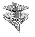
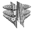
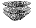
a) b) c) d)

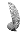
Figure 4: Grafting and earthquake construction in the lightcone for a single geodesic:
a) Intersection of lightcone with the plane defined by the geodesic
b) Cutting the lightcone and shifting the pieces in the grafting construction
c) Deformed domain for the grafting construction.
d) Earthquake on a constant cosmological time surface

In the earthquake construction, one proceeds analogously. As in the case of grafting, one selects a basepoint and cuts the lightcone along all planes defined by geodesics in the multicurve. One then applies Lorentz boosts to the pieces that do not contain the basepoint. These boosts are chosen such that they preserve the associated planes and have the weight $w\in\mathbb{R}^{+}$ as their rapidity. Their action on the hyperboloids is depicted in Figure 4 d). They preserve the domain $\tilde{M}$ and its foliation by constant cosmological time surfaces $\tilde{M}_{T}$. The resulting spacetime remains conformally static.

3.2 Action of grafting and earthquake on the holonomies

The action of the fundamental group $\pi_{1}(M)$ on the deformed domains via the holonomies $h:\pi_{1}(M)\rightarrow P_{3}$ is defined in such a way that it identifies two points in the deformed domain if and only if the corresponding points in the original lightcone were identified. In the case of a grafted spacetime, this implies that the holonomies acquire a non-trivial translational component that takes into account the translations and grafted strips. Grafting therefore does not affect the Lorentzian components of the holonomies, which determine the Fuchsian group $\Gamma$, but changes their translational components. For the spacetimes deformed by earthquakes, the translational components of the holonomies remain trivial, but the Lorentzian components change to take into account the Lorentz boosts applied to different pieces of the lightcone.

The transformation of the holonomies associated with grafting and earthquakes can be determined explicitly. As the holonomies characterise the spacetime uniquely, it follows that grafting and earthquakes induce transformations on the phase space $\mathcal{P}$ (2.5). These phase space transformations are given explicitly in [2, 3, 4].

3.3 Spacetimes

The deformed spacetimes obtained via the grafting and earthquake construction are given as the quotients of the deformed domains by the action of the fundamental group via the holonomies $h:\pi_{1}(M)\rightarrow P_{3}$. In the case of a grafted spacetime, one finds that the resulting spacetimes are no longer conformally static, but show a non-trivial evolution with the cosmological time as indicated in Figure 5. While the constant cosmological time surfaces of a conformally static spacetime are all copies of the same Riemann surface $\Sigma={\mathbb{H}^{2}}/\Gamma$, rescaled by the cosmological time, this is no longer true for the grafted spacetimes. Although the part outside the grafted strips is rescaled with the cosmological time, the width of the grafted strips remains constant. This implies that the impact of grafting is maximal near the initial singularity and vanishes in the limit $T\rightarrow\infty$ as shown in Figure 5.

The grafting construction thus maps the conformally static spacetime associated with a cocompact Fuchsian group $\Gamma$ to an evolving spacetime associated with $\Gamma$, which approaches the conformally static spacetime in the limit $T\rightarrow\infty$. In contrast, the earthquake preserves the constant cosmological time surfaces and affects only the Lorentzian component of the holonomies. It maps a conformally static spacetime associated with a Fuchsian group $\Gamma$ to a conformally static spacetime associated with a non-equivalent Fuchsian group $\Gamma^{\prime}$.

Figure 5: Evolution of the surfaces $M_{T}$ in a conformally static and grafted spacetime.

4 Geometry transformations and observables

As the fundamental diffeomorphism invariant observables of the theory which characterise the geometry of the spacetimes and parametrise the phase space $\mathcal{P}$ (2.5), the Wilson loop observables play an important role in quantisation. This makes it natural to investigate the geometrical interpretation of the mass and spin observables (2.6). It also raises the question how the phase space transformations that are generated by these observables via the Poisson bracket affect the geometry of the spacetime.

Theorem 4.1

[3, 4] Let $M\approx\mathbb{R}\times S$ be a a conformally static vacuum spacetime of genus $g\geq 2$ and $\lambda$ a closed, simple geodesic on a constant cosmological time surface $M_{T}$ with associated weight $w$. Then the two fundamental Wilson loop observables, the mass $m_{\lambda}$ and spin $s_{\lambda}$, associated to $\lambda$ generate via the Poisson bracket the phase space transformations $\text{Gr}_{\lambda}^{w},E_{\lambda}^{w}:\mathcal{P}\rightarrow\mathcal{P}$ associated with geometry change through grafting and earthquake along $\lambda$

$$\{m_{\lambda},f\}=\frac{d}{dw}\bigg{|}_{w=0}f\circ\text{Gr}_{\lambda}^{w}\qquad\qquad\{s_{\lambda},f\}=\frac{d}{dw}\bigg{|}_{w=0}f\circ\text{E}_{\lambda}^{w}\qquad\forall f\in\mathcal{C}^{\infty}(\mathcal{P}).$$ (4.1)

This theorem confirms that the Wilson loop observables which are fundamental in the quantisation of the theory also play a distinguished role with respect to spacetime geometry: they generate via the Poisson bracket the two fundamental transformations which change the geometry of the spacetime. In particular, this implies that the grafting and earthquake transformations are Poisson isomorphisms (canonical transformations).

It also provides one with a clear physical interpretation of the two fundamental Wilson loop observables which justifies the names “mass” and “spin”. The mass observable generates grafting, the spin observable earthquakes, which can be viewed, respectively, as a translation and a rotation associated with a geodesic. In analogy with classical mechanics, where momenta generate translations and angular momenta rotations, the mass and spin observable can thus be interpreted as a momentum and an angular momentum of a geodesic.

5 Measurements associated with returning lightrays

Although the geometry of Lorentzian vacuum (2+1)-spacetimes is well-understood, it has been difficult to obtain interesting physics from the theory. This is due to the fact that it is not readily apparent how the variables which parametrise the phase space, holonomies and Wilson loops, could be measured by an observer in the spacetime. Moreover, it is not obvious what physically meaningful measurement an observer could make in an empty spacetime and how such measurements would allow him to distinguish the different spacetimes that are all locally isometric to Minkowski space.

This problem is addressed in [5], where it is shown that an observer can determine the geometry of such spacetimes by sending out lightrays which return to him at a later time. The observer can then measure the return time, the eigentime elapsed between the emission of the lightray and its return. He can determine into which directions the light needs to be sent in order to return, and he can compare the frequencies of the emitted and returning lightray.

To obtain explicit expressions for these measurements in terms of the holonomy variables, it is advantageous to work in the universal cover $\tilde{M}\subset\mathbb{M}^{3}$. We start by explaining how the relevant concepts (observers, lightrays, returning lightrays) are implemented in this description. By definition, an observer in free fall in $M$ is characterised by a timelike, future oriented geodesic $g:[0,\infty)\rightarrow M$. This corresponds to a $\pi_{1}(M)$-equivalence class of timelike, future directed geodesics in the universal cover $\tilde{M}$. This equivalence class of geodesics is obtained by taking one lift $\tilde{g}:[0,\infty)\rightarrow\tilde{M}$ of $g$ to $\tilde{M}$ and constructing its images $h(\lambda)\tilde{g}$, $\lambda\in\pi_{1}(M)$ under the holonomies as shown in Figure 6.

A lightray is characterised by lightlike geodesic in $M$ or, equivalently, the $\pi_{1}(M)$-equivalence class of lightlike, future oriented geodesics in $\tilde{M}$ obtained by taking one lift and acting on it with the holonomies. A returning lightray with respect to an observer with wordline $g:[0,\infty)\rightarrow M$ is a lightray in $M$ that intersects the worldline of the observer twice. In the universal cover, such a returning lightray can be described as the $\pi_{1}(M)$-equivalence class of a lightlike geodesic $\tilde{M}\subset\mathbb{M}^{3}$ that starts at one lift $\tilde{g}:[0,\infty)\rightarrow\tilde{M}$ of the observer’s worldline and ends at one if its images $h(\lambda)\tilde{g}$, $\lambda\in\pi_{1}(M)$, as shown in Figure 6.

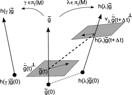
Figure 6: Returning lightray in the universal cover $\tilde{M}\subset\mathbb{M}^{3}$

As the universal cover $\tilde{M}$ is a region in Minkowski space, the lifts of the observer’s wordline and of lightrays are straight lines in Minkowski space with, respectively, timelike and lightlike tangent vectors. The return time $\Delta t$ is then obtained by parametrising the observer’s worldline $g:[0,\infty)\rightarrow M$ and its lifts $\tilde{g}:[0,\infty)\rightarrow\tilde{M}$ according to eigentime and determining the unique positive solution of the quadratic equation

$$\eta\big{(}\,h(\lambda)\tilde{g}(t+\Delta t)-\tilde{g}(t)\,,\,h(\lambda)\tilde{g}(t+\Delta t)-\tilde{g}(t)\,\big{)}=0.$$ (5.1)

Returning lightrays are thus in one-to-one correspondence with elements of $\pi_{1}(M)$. The directions into which the returning lightray associated with an element $\lambda\in\pi_{1}(M)$ is emitted and from which it returns are given by the projection of the lightlike vector $h(\lambda)\tilde{g}(t+\Delta t)-\tilde{g}(t)$ on the orthogonal complement of, respectively, the tangent vector $\dot{\tilde{g}}(t)\in\mathbb{R}^{3}$ and $v_{\lambda}\dot{\tilde{g}}(t+\Delta t)$, where $h(\lambda)=(v_{\lambda},{\mbox{\boldmath$a$}}_{\lambda})$. The relative frequencies of the emitted and returning lightray can be determined in analogy to the relativistic Doppler effect. One obtains

$$\frac{f_{r}}{f_{e}}=\frac{\eta\big{(}\,h(\lambda)\tilde{g}(t+\Delta t)-\tilde{g}(t)\,,\,v_{\lambda}\dot{\tilde{g}}(t)\,\big{)}}{\eta\big{(}\,h(\lambda)\tilde{g}(t+\Delta t)-\tilde{g}(t)\,,\,\dot{\tilde{g}}(t)\,\big{)}}.$$ (5.2)

Using these definitions, one can derive explicit expressions for the return time, the directions and the relative frequency shift [5].

Theorem 5.1

[5] Let $\tilde{g}:[0,\infty)\rightarrow\tilde{M}$ be the lift of the worldline of an observer in free fall in $M$, parametrised according to eigentime:

$$\tilde{g}(t)=t{\mbox{\boldmath$x$}}+{\mbox{\boldmath$x$}}_{0}\qquad\text{with}\qquad{\mbox{\boldmath$x$}}\in\mathbb{R}^{3},{\mbox{\boldmath$x$}}^{2}=-1,x^{0}>0,{\mbox{\boldmath$x$}}_{0}\in\tilde{M}.$$ (5.3)

Consider the returning lightray associated with an element $\lambda\in\pi_{1}(M)$ that is emitted by the observer at eigentime $t$ and returns to him at $t+\Delta t$. Then the return time $\Delta t$ is given by

$$\Delta t=(t+\sigma_{\lambda})(\cosh\rho_{\lambda}-1)-\tau_{\lambda}+\sinh\rho_{\lambda}\sqrt{(t+\sigma_{\lambda})^{2}+\nu_{\lambda}^{2}},$$ (5.4)

where $\rho_{\lambda}=-{\mbox{\boldmath$x$}}\cdot(v_{\lambda}{\mbox{\boldmath$x$}})$ and $h(\lambda){\mbox{\boldmath$x$}}_{0}-{\mbox{\boldmath$x$}}_{0}=\sigma_{\lambda}(v_{\lambda}{\mbox{\boldmath$x$}}-{\mbox{\boldmath$x$}})+\tau_{\lambda}v_{\lambda}{\mbox{\boldmath$x$}}+\nu_{\lambda}\,{\mbox{\boldmath$x$}}\wedge v_{\lambda}{\mbox{\boldmath$x$}}$. The direction into which the lightray is emitted is given by the spacelike unit vector

$$\hat{\mbox{\boldmath$p$}}^{e}_{\lambda}\!=\!\cos\phi_{e}\;\frac{v_{\lambda}{\mbox{\boldmath$x$}}\!+\!({\mbox{\boldmath$x$}}\cdot v_{\lambda}{\mbox{\boldmath$x$}}){\mbox{\boldmath$x$}}}{|v_{\lambda}{\mbox{\boldmath$x$}}\!+\!({\mbox{\boldmath$x$}}\cdot v_{\lambda}{\mbox{\boldmath$x$}}){\mbox{\boldmath$x$}}|}\!+\!\sin\phi_{e}\;\frac{{\mbox{\boldmath$x$}}\wedge v_{\lambda}{\mbox{\boldmath$x$}}}{|{\mbox{\boldmath$x$}}\wedge v_{\lambda}{\mbox{\boldmath$x$}}|}\;\;\text{with}\;\;\tan\phi_{e}\!=\!\frac{\nu_{\lambda}}{\sinh\rho_{\lambda}\sqrt{(t\!+\!\sigma_{\lambda})^{2}\!+\!\nu_{\lambda}^{2}}},$$ (5.5)

and the relative frequency $f_{r}/f_{e}$ of the lightray at its emission and return are given by

$$f_{r}/f_{e}=\frac{\sqrt{(t+\sigma_{\lambda})^{2}+\nu_{\lambda}^{2}}}{\cosh\rho_{\lambda}\sqrt{(t+\sigma_{\lambda})^{2}+\nu_{\lambda}^{2}}+\sinh\rho_{\lambda}(t+\sigma_{\lambda})}<1.$$ (5.6)

The physical interpretation of these measurements is discussed in detail in [5]. It is shown there that for an observer in a conformally static spacetime whose eigentime coincides with the cosmological time, the relative frequencies and the directions of emission do not vary with time and the return time is a linear function of the emission time. This is the case for a general observer in a general spacetime in the limit where the emission time $t$ and hence the cosmological time $T$ tend to infinity. In this limit the effect of grafting becomes negligible and the grafted spacetime approaches the associated conformally static spacetime.

The measurements in Theorem 5.1 thus allow an observer to draw conclusions about the geometry of the underlying spacetime. This raises the question if an observer can use them to determine the full geometry of the spacetime in finite eigentime. In other words: can an observer determine the holonomies $h(\lambda)$ for a set of generators of the fundamental group $\pi_{1}(M)$ up to conjugation in finite eigentime based on such measurements? It is shown in [14, 15] that this is indeed possible. By considering an observer who emits light in all directions at a given time and measures the return time and return direction for each returning lightray, one obtains a procedure that yields the holonomies (up to conjugation) from a finite number of returning lightrays [14, 15]. The measurements thus allow an observer to determine the associated point in phase space $\mathcal{P}$ (2.5) and the full geometry of the spacetime in finite eigentime.

Acknowledgements

I thank the organisers of 2nd School and Workshop on Quantum Gravity and Quantum Geometry (Corfu, 13-20/09/2009), where this work was presented as a talk. My research is supported by the Emmy Noether fellowship ME 3425/1-1 of the German Research Foundation (DFG).

References

- [1] Carlip S 1998 Quantum gravity in 2+1 dimensions (Cambridge: Cambridge University Press)
- [2] Benedetti R, Bonsante F 2009 Canonical Wick rotations in 3-dimensional gravity, AMS Memoirs 926, Vol 198.
- [3] Meusburger C 2006 Grafting and Poisson structure in (2+1)-gravity with vanishing cosmological constant, Commun. Math. Phys. 266 735–775.
- [4] Meusburger C 2007 Geometrical (2+1)-gravity and the Chern-Simons formulation: Grafting, Dehn twists, Wilson loop observables and the cosmological constant, Commun. Math. Phys. 273 705–754.
- [5] Meusburger C 2009 Cosmological measurements, time and observables in (2+1)-dimensional gravity, Class. Quant. Grav. 26 055006.
- [6] Mess G 2007 Lorentz spacetimes of constant curvature, preprint IHES/M/90/28 (1990), Geometriae Dedicata 126:1 3–45.
- [7] Andersson L, Barbot T, Benedetti R, Bonsante F, Goldman W M, Labourie F, Scannell K P, Schlenker J-M 2007 Notes on a paper of Mess, Geometriae Dedicata 126:1 47–70.
- [8] Barbot T 2005 Globally hyperbolic flat spacetimes, Journ. Geom. Phys. 53 123–165.
- [9] Franzosi R, Guadagnini E 1996 Topology and classical geometry in (2 + 1) gravity, Class. Quant. Grav. 13 433–460.
- [10] Benedetti R, Guadagnini E 2001 Cosmological time in (2+1)-gravity, Nucl. Phys. B 613 330–352.
- [11] Goldman W 1984 The symplectic nature of fundamental groups of surfaces, Adv. in Math. 54:2, 200–225.
- [12] Thurston W P 1987 Earthquakes in two-dimensional hyperbolic geometry. In Epstein DB (edt) Low dimensional topology and Kleinian groups (Cambridge: Cambridge University Press) 91–112.
- [13] McMullen C 1998 Complex Earthquakes and Teichmüller theory, J. Amer. Math. Soc. 11 283–320.
- [14] Meusburger C 2009 Global Lorentzian geometry from lightlike geodesics: What does an observer in (2+1)-gravity see?, arXiv:1001.1842 [math-ph].
- [15] Meusburger C 2009 Spacetime geometry in (2+1)-gravity via measurements with returning lightrays, AIP Conf. Proc. 1196 181–189.