Magnetic fields and spiral arms in the galaxy M51

Abstract

We use new multi-wavelength radio observations, made with the VLA and Effelsberg telescopes, to study the magnetic field of the nearby galaxy M51 on scales from $200\,\mathrm{pc}$ to several $\,\mathrm{kpc}$. Interferometric and single dish data are combined to obtain new maps at $\lambda\lambda 3,6\,\mathrm{cm}$ in total and polarized emission, and earlier $\lambda 20\,\mathrm{cm}$ data are re-reduced. We compare the spatial distribution of the radio emission with observations of the neutral gas, derive radio spectral index and Faraday depolarization maps, and model the large-scale variation in Faraday rotation in order to deduce the structure of the regular magnetic field. We find that the $\lambda 20\,\mathrm{cm}$ emission from the disc is severely depolarized and that a dominating fraction of the observed polarized emission at $\lambda 6\,\mathrm{cm}$ must be due to anisotropic small-scale magnetic fields. Taking this into account, we derive two components for the regular magnetic field in this galaxy: the disc is dominated by a combination of azimuthal modes, $m=0+2$, but in the halo only an $m=1$ mode is required to fit the observations. We disuss how the observed arm-interarm contrast in radio intensities can be reconciled with evidence for strong gas compression in the spiral shocks. In the inner spiral arms, the strong arm–interarm contrasts in total and polarized radio emission are roughly consistent with expectations from shock compression of the regular and turbulent components of the magnetic field. However, the average arm–interam contrast, representative of the radii $r>2\,\mathrm{kpc}$ where the spiral arms are broader, is not compatible with straightforward compression: lower arm–interarm contrasts than expected may be due to resolution effects and decompression of the magnetic field as it leaves the arms. We suggest a simple method to estimate the turbulent scale in the magneto-ionic medium from the dependence of the standard deviation of the observed Faraday rotation measure on resolution. We thus obtain an estimate of $50\,\mathrm{pc}$ for the size of the turbulent eddies.

1 Introduction

The Whirlpool galaxy, M51 or NGC 5194, is one of the classical grand-design spiral galaxies. The two spiral arms of M51 can be traced through more than 360° in azimuthal angle in numerous wavebands. M51 is probably perturbed by a recent encounter with its companion galaxy NGC 5195. Such interactions usually result in enhanced star formation, either localized or global, as tidal forces and density waves compress the interstellar medium. In M51 this may have resulted in two systems of density waves (Elmegreen et al., 1989).

M51 was the first external galaxy where polarized radio emission was detected (, Mathewson et al.1972) and one of the few external galaxies where optical polarization has been studied (Scarrott et al., 1987). Neininger (1992) and Horellou et al. (1992) found that the lines of the regular magnetic field in M51 have a spiral shape, but their resolution was too low to determine how well the field is aligned with the optical spiral arms. Horellou et al. (1992) realized that, at wavelengths of $\lambda\geq 18$ cm, only polarized emission from a foreground layer reaches the observer because of Faraday depolarization, and the Faraday rotation measures obtained at the longer wavelengths are much smaller than those at shorter wavelengths. Heald et al. (2009) observed a fractional polarization at $\lambda 22\,\mathrm{cm}$ of around $5\%$ in the optical disc, increasing to $30\%$ at large radii, and Faraday rotation measures of a similar magnitude to those found by Horellou et al. (1992). Berkhuijsen et al. (1997) analyzed the global magnetic field of M51 using radio data at four frequencies and found that the average orientation of the fitted magnetic field is similar to the average pitch angle of the optical spiral arms measured by Howard & Byrd (1990). Berkhuijsen et al. (1997) represented the magnetic field in the disc of M51 as a superposition of periodic azimuthal modes, with about equal contribution from the axisymmetric $m=0$ and the bisymmetric $m=1$ ones. Their fit contains a magnetic field reversal at about 5 kpc radius which extends over a few kpc in azimuth. Furthermore, Berkhuijsen et al. (1997) found evidence for an axisymmetric magnetic field in the halo of M51 (visible at $\lambda 18\,\mathrm{cm}$ and $\lambda 20\,\mathrm{cm}$) with a reversed direction (inwards) with respect to the axisymmetric mode of the disc field (outwards).

The results of Berkhuijsen et al. (1997) indicate that the magnetic field of M51 is strong and partly regular, with some interesting properties. However, some of their results may be affected by the low angular resolution which was limited by the Effelsberg single-dish data at $\lambda 2.8\,\mathrm{cm}$. Furthermore, no correction for missing large-scale structure could be applied to the VLA $\lambda 6\,\mathrm{cm}$ polarization data because no single-dish map was available at that time.

Here we present a refined analysis based on new data with higher resolution and better sensitivity. Our new surveys of M51 in total and linearly polarized $\lambda 3\,\mathrm{cm}$ and $\lambda 6\,\mathrm{cm}$ radio continuum emission combines the resolution of the VLA with the sensitivity of the Effelsberg single-dish telescope. The new maps are of comparable resolution to the maps of the CO(1–0) emission (Helfer et al., 2003) and mid-infrared dust emission (Sauvage et al., 1996; Regan et al., 2006) and are of unprecedented sensitivity. The shape of the spiral radio arms and the comparison to the arms seen with different tracers were discussed in a separate paper (Patrikeev et al., 2006).

The spiral shocks in M51 are strong and regular (Aalto et al., 1999) and offer the possibility to compare arm–interarm contrasts of gas and the magnetic field. We analyse our new data to try to separate the contribution to the observed polarized emission from regular (or mean) magnetic fields and anisotropic random magnetic fields produced by compression and/or shear in the spiral arms.

The new high-resolution polarization maps allow us for the first time to investigate in detail the interaction between the magnetic fields and the shock fronts. Results from the barred galaxies NGC 1097 and NGC 1365 showed that the small-scale and the large-scale magnetic field components behave differently, i.e. the small-scale field is compressed significantly in the bar’s shock, while the large-scale field is hardly compressed (Beck et al., 2005). This was interpreted as a strong indication that the large-scale field is coupled to the warm, diffuse gas which is only weakly compressed. We investigate whether a similar decoupling of the regular magnetic field from the dense gas clouds is suggested by the observed arm–interarm contrast in M51.

The basic parameters we adopt for M51 are: centre’s right ascension $\mathrm{1}3^{\mathrm{h}}29^{\mathrm{m}}52\aas@@fstack{s}709$ and declination (J2000) $+47\degr 11\arcmin 42\aas@@fstack{\prime\prime}59$ (Ford et al., 1985); distance 7.6 Mpc, (Ciardullo et al., 2002), thus $1"\approx 37\,\mathrm{pc}$; position angle of major axis $-10\degr$ ($0\degr$ is North) and inclination $-20\degr$ ($0\degr$ is face-on) (Tully, 1974). The inclination is measured from the galaxy’s rotation axis to the line-of-sight, viewed from the northern end of the major axis, and its sign is important for the geometry of the model discussed in Sect. 6.

2 Observations and data reduction

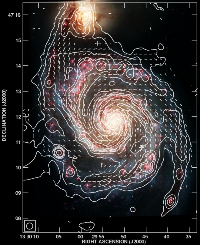
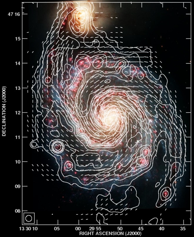
Figure 1: (a) $\lambda 3\,\mathrm{cm}$ and (b) $\lambda 6\,\mathrm{cm}$ radio emission at $15\arcsec$ resolution from VLA and Effelsberg observations, overlaid on a Hubble Space Telescope optical image (image credit: NASA, ESA, S. Beckwith (STScI), and The Hubble Heritage Team (STScI/AURA)). Total intensity contours in both maps are at $6,12,24,36,48,96,192$ times the noise levels of $20\,\mu\mathrm{Jy/beam}$ at $\lambda 3\,\mathrm{cm}$ and $30\,\mu\mathrm{Jy/beam}$ at $\lambda 6\,\mathrm{cm}$. (Note that the roughly horizontal contours at the left edge of panel (a) are artefacts arising from mosaicing the two VLA pointings.) Also shown are the $B$-vectors of polarized emission: the plane of polarization of the observed electric field rotated by 90°, not corrected for Faraday rotation, with a length proportional to the polarized intensity ($PI$) and only plotted where $PI\geq 3\sigma_{PI}$.

2.1 VLA observations

M51 was observed in October 2001 at $\lambda 3.5\,\mathrm{cm}$ with the VLA in the compact D configuration and in August 2001 at $\lambda 6.2\,\mathrm{cm}$ in the C configuration. Two pointings of the array, at the northern and southern parts of the galaxy, were required to obtain complete coverage of M51 at $\lambda 3.5\,\mathrm{cm}$. The data were edited, calibrated and imaged using standard AIPS procedures and VLA calibration sources. After initial examination of the data and the flagging of bad visibilities, self-calibration was used. After correction for the pattern of the primary beam the two pointings at $\lambda 3.5\,\mathrm{cm}$ were mosaiced using the AIPS task LTESS. The calibrated $\lambda 6.2\,\mathrm{cm}$ C-array uv-data were combined with existing $\lambda 6.2\,\mathrm{cm}$ D-array data (Neininger & Horellou, 1996).

A new $\lambda 20\,\mathrm{cm}$ map in total power and polarization is presented in Fig. 3, based on the C-array data of Neininger & Horellou (1996) combined with D-array data of Horellou et al. (1992). All of the observations were re-reduced for this work, the two data sets were combined and then smoothed to a resolution of $15\arcsec$ to improve the signal-to-noise ratio. The resulting maps at $\lambda 20\,\mathrm{cm}$ contain information on all scales down to the beamsize as the primary beam of the VLA at $\lambda 20\,\mathrm{cm}$ in the D-array is $\sim 30\arcmin$, about twice the size of M51 on the sky.

Different weighting schemes were used in the final imaging of the data to produce maps with either high resolution (natural weighting) or high signal-to-noise (uniform weighting) and for a compromise between the two extremes (robust weighting, obtained by setting the parameter ROBUST=0 in the AIPS task IMAGR). Maps of the Stokes parameters $I$, $Q$ and $U$ were produced in each case. The optimum number of iterations of the CLEAN algorithm used to produce the images was determined individually for each map. Following slight smoothing, the $Q$ and $U$ maps were combined to give the polarized intensity $PI=\sqrt{Q^{2}+U^{2}}$, using a first-order correction for the positive bias (Wardle & Kronberg, 1974).

Table 1: The merged VLA and Effelsberg maps discussed in this paper, their half-power beam widths, imaging weighting schemes and their r.m.s. noises in total and polarized emission, $\sigma_{I}$ and $\sigma_{PI}$, respectively

$\lambda$	HPBW	Weighting	$\sigma_{I}$	$\sigma_{PI}$
(cm)			($\,\mu\mathrm{Jy/beam}$)	($\,\mu\mathrm{Jy/beam}$)
23	18″	robust	$12$	$10$
23	15″	natural	$20$	$\phantom{1}8$
26	14″	uniform	$15$	$10$
26	18″	robust	$25$	$10$
26	15″	natural	$30$	$10$
20	15″	natural	$20$	$13$

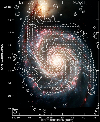
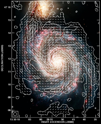
Figure 2: (a) $\lambda 3\,\mathrm{cm}$ and (b) $\lambda 6\,\mathrm{cm}$ (right) polarized radio emission at $15\arcsec$ resolution from VLA and Effelsberg observations, overlaid on the same optical image as in Fig. 1. Polarized intensity contours in both maps are at $3,9,15,21$ times the noise level of $8\,\mu\mathrm{Jy/beam}$ at $\lambda 3\,\mathrm{cm}$ and $10\,\mu\mathrm{Jy/beam}$ at $\lambda 6\,\mathrm{cm}$. Also shown are the $B$-vectors of polarized emission: the position angle of the polarized electric field rotated by 90°, not corrected for Faraday rotation, with the length proportional to the polarized intensity $PI$ and only plotted where $P\geq 3\sigma_{PI}$.

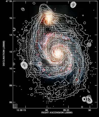
Figure 3: Contours of $\lambda 20\,\mathrm{cm}$ total radio emission at $15\arcsec$ resolution, overlaid on the same optical image as in Fig. 1. Total intensity contours are at 6, 12, 24, 36, 48, 96, 192 times the noise level of $20\,\mu\mathrm{Jy/beam}$. Also shown are the $B$-vectors of polarized emission: the plane of polarization of the observed electric field rotated by 90°, not corrected for Faraday rotation, with a length proportional to the polarized intensity $PI$ and only plotted where $PI\geq 3\sigma_{PI}$.

2.2 Effelsberg observations and merging

In order to correct the VLA maps at $\lambda 3\,\mathrm{cm}$ for missing extended emission we made observations of M51 in total intensity and polarization with the 100-m Effelsberg telescope in December 2001 and April 2002 using the sensitive $\lambda 3.6\,\mathrm{cm}$ (1.1 GHz bandwidth) receiver. We obtained 44 maps of a 12$\arcmin$ by 12$\arcmin$ field around M51, scanned in orthogonal directions. Each map in $I$, $Q$ and $U$ was edited and baseline corrected individually, then all maps in each Stokes parameter were combined using a basket weaving method (Emerson & Gräve, 1988). The r.m.s. noise in the final maps, after slight smoothing to $90\arcsec$, is $200\,\mu\mathrm{Jy/beam}$ in total intensity and $20\,\mu\mathrm{Jy/beam}$ in polarized intensity.

At $\lambda 6.2\,\mathrm{cm}$, ten maps of a 41$\arcmin$ by 34$\arcmin$ field were observed in November 2003 with the 4.85 GHz (500 MHz bandwidth) dual-horn receiver. The combined data resulted in a new $180\arcsec$ resolution image with r.m.s. noise of $250\,\mu\mathrm{Jy/beam}$ in total intensity and $25\,\mu\mathrm{Jy/beam}$ in polarization.

Maps from the VLA and Effelsberg were combined using the AIPS task IMERG. A useful description of the principles of merging single dish and interferometric data is given by Stanimirovic (2002). The range of overlap in the uv plane between the two images (parameter uvrange in IMERG) was estimated as follows: we assumed an effective Effelsberg diameter of about 60 m to estimate the maximum extent of the single dish in the uv space ($1.7\,\mathrm{k}\lambda$ at $\lambda 3.6\,\mathrm{cm}$ and $1.0\,\mathrm{k}\lambda$ at $\lambda 6.2\,\mathrm{cm}$) and used the minimum separation of the VLA antennas in the D-array configuration, $35$ m, to calculate the minimum coverage of the interferometer in the uv space ($1.0\,\mathrm{k}\lambda$ at $\lambda 3.6\,\mathrm{cm}$ and $0.6\,\mathrm{k}\lambda$ at $\lambda 6.2\,\mathrm{cm}$). We then varied these parameters in order to find the optimum overlap in the uv space by comparing the integrated total flux in the merged maps with that of the single dish maps; the optimal uv-ranges for merging were found to be $1.0\rightarrow 1.6\,\mathrm{k}\lambda$ at $\lambda 3.6\,\mathrm{cm}$ and $0.5\rightarrow 0.7\,\mathrm{k}\lambda$ at $\lambda 6.2\,\mathrm{cm}$. Merging of the $Q$ and $U$ maps was carried out using the same optimum uv range as found for $I$.

The fraction of total emission (Stokes $I$) present in the VLA maps – those produced using natural weighting, and hence with the highest signal-to-noise ratio – is about 30% at $\lambda 3\,\mathrm{cm}$ and close to 50% at $\lambda 6\,\mathrm{cm}$ compared to the merged maps. Small-scale fluctuations in $Q$ and $U$ due to variations in the magnetic field orientation and Faraday rotation in M51 mean that the polarized emission is less severely affected by missing large-scales (alternatively, the single dish detects the large-scale emission missed by an interferometer but simultaneously suffers from stronger wavelength-independent beam depolarization). At $\lambda 3\,\mathrm{cm}$ the VLA map contains about 75% of the polarized emission present in the merged map, with about 85% present at $\lambda 6\,\mathrm{cm}$.

Following the merging, the maps in $I$, $Q$ and $U$ were convolved with a Gaussian beam to give a slightly coarser resolution and higher signal-to-noise ratio. The maps that are discussed in this paper are listed in Table 1 along with the r.m.s. noises in total and polarized intensity.

3 The M51 maps

3.1 The spiral arms of M51 as seen in radio emission

Figure 1 shows the total radio continuum emission and the $B$-vectors of polarized emission (the observed plane of linear polarization rotated by 90°) at $\lambda 3\,\mathrm{cm}$ and $\lambda 6\,\mathrm{cm}$, overlaid on a Hubble Space Telescope optical image. At the assumed distance of 7.6 Mpc, the $15\arcsec$ resolution corresponds to $560\,\mathrm{pc}$ and $590\,\mathrm{pc}$ along the major and minor axes, respectively. The distribution of polarized emission at $\lambda\lambda 3,6\,\mathrm{cm}$ is shown in Fig. 2 at $15\arcsec$ resolution. The extensive $\lambda 20\,\mathrm{cm}$ total emission disc is shown in Fig. 3 also at $15\arcsec$ resolution.

The total emission at $\lambda 3\,\mathrm{cm}$ and $\lambda 6\,\mathrm{cm}$ in Fig. 1 shows a close correspondence with the optical spiral arms whereas the $\lambda 20\,\mathrm{cm}$ total emission (Fig. 3) and $\lambda 3\,\mathrm{cm}$ and $\lambda 6\,\mathrm{cm}$ polarized emission (Fig. 2) are spread more evenly across the galactic disc. Compact, bright peaks of total emission coincide with complexes of H ii regions in the spiral arms, as expected if thermal bremsstrahlung is a significant component of the radio signal at these peaks. The flatter spectral index ($\alpha\lesssim 0.6$ where $I\propto\nu^{-\alpha}$, Fig. 7) and the absence of the corresponding peaks in polarized radio emission (Fig. 2) suggest that a significant proportion of the centimeter wavelength radio emission in these peaks is thermal. The extended $\lambda 20\,\mathrm{cm}$ total emission and $\lambda 3\,\mathrm{cm}$ and $\lambda 6\,\mathrm{cm}$ polarized emission accurately trace the synchrotron component of the radio continuum.

Ridges of enhanced polarized emission are prominent in the inner galaxy; some are located on the optical spiral arms but others are located in-between the arms. A detailed analysis of the location and pitch angles of the spiral arms traced by different observations and a comparison of the pitch angles with the orientation of the regular magnetic field is given by Patrikeev et al. (2006). They find systematic shifts between the spiral ridges seen in polarized and total radio emission, integrated CO line emission and infrared emission, which are consistent with the following sequence in a density wave picture: firstly, shock compresses gas and magnetic fields (traced by polarized radio emission), then molecules are formed (traced by CO) and finally thermal emission is generated (traced by infrared). Patrikeev et al. (2006) also show that while the pitch angle of the regular magnetic field is fairly close to that of the gaseous spiral arms at the location of the arms, the magnetic field pitch angle changes from the above by around $\pm 15\degr$ in interarm regions.

3.2 The connection between polarized radio emission and gaseous spiral arms

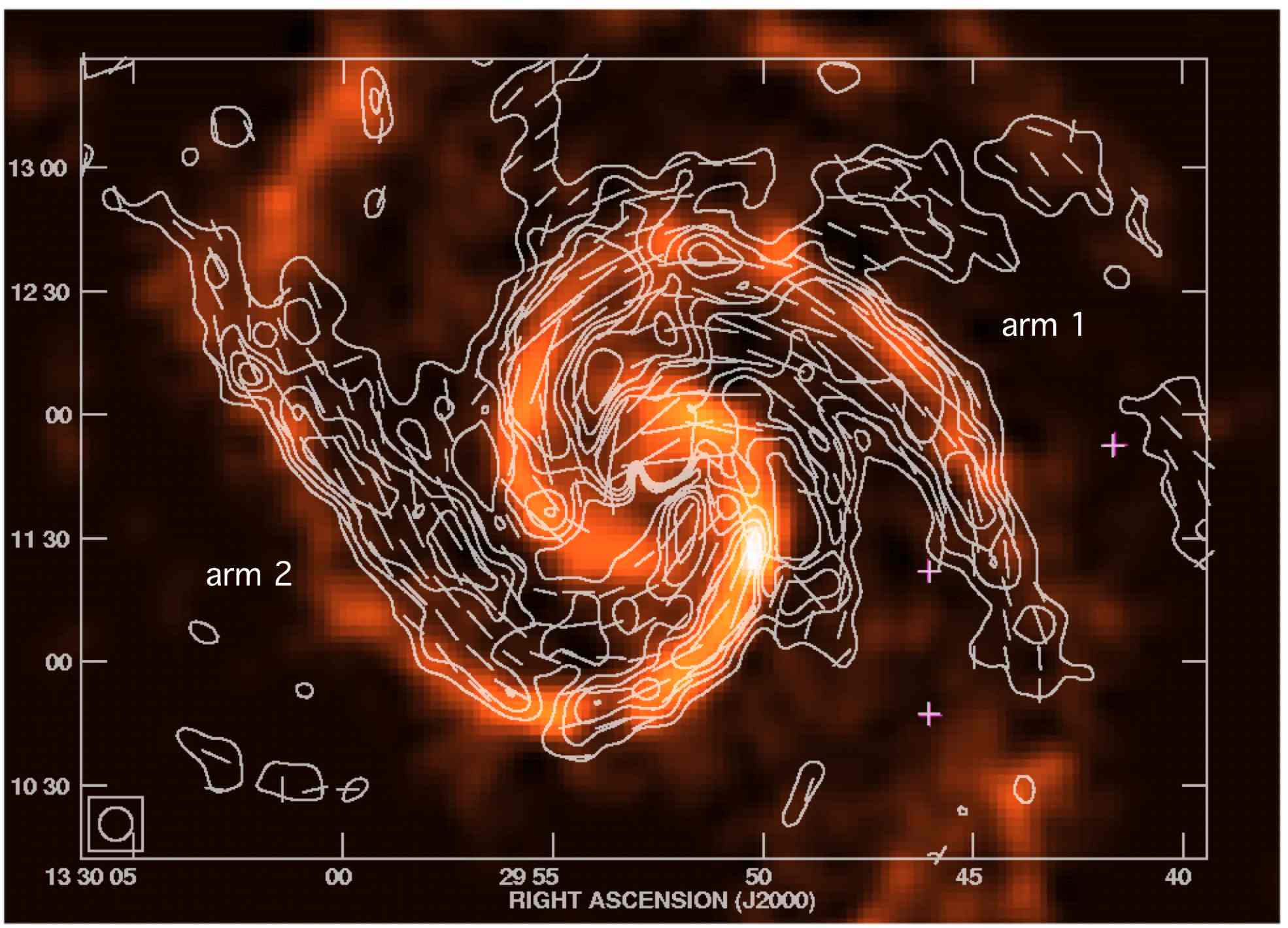
Figure 4: Contours of the $\lambda 6\,\mathrm{cm}$ polarized radio emission (VLA and Effelsberg combined) in the central $\sim 3\arcmin\times 4\arcmin$ of M51 at $8\arcsec$ resolution, along with Faraday-rotation corrected B-vectors, overlaid on the map of integrated CO(1–0) line emission of Helfer et al. (2003). Contours are at $3,5,7,9$ times the noise level of $10\,\mu\mathrm{Jy/beam}$.

In Fig. 4, the $\lambda 6\,\mathrm{cm}$ polarized emission and the orientation of the regular magnetic field in the central $8\,\mathrm{kpc}$ of M51 are overlaid onto an image of the spiral arms as traced by the CO(1–0) integrated line emission. Part of the polarized emission appears to be concentrated in elongated arm-like structures that sometimes coincide with the gas spiral.

The correspondence between polarized and CO arms is good along most of the northern arm in Fig. 4 (called Arm 1 in the rest of the paper) and in the inner part of the southern arm (called Arm 2). Arm 1 continues towards the south where the polarized emission longer coincides with the CO and optical arms, but becomes broader further out (Fig. 2).

Moving along Arm 2, the excellent overlap of the radio polarization and CO in the inner arm ends abruptly further in the south (Fig. 4), beyond which the distribution of polarized emission is very broad and located on the galactic centre side of the gaseous spiral arm: the peak of this interarm polarized emission corresponds very closely with the pronounced peaks in radial velocity, $v_{r}\simeq 100\,\mathrm{km\,s^{-1}}$, derived by Shetty et al. (2007) (shown in their Fig. 14). This may be an indication that strong shear in the interarm gas flow is producing this magnetic feature. At about 6 kpc radius, the polarization Arm 2 crosses the CO and optical arms in the east, followed in the northeast by a bending away from the optical arm towards the companion galaxy NGC 5195 (Fig. 2). The northern part of Arm 2 is weakly polarized and rather irregular in total and CO emission. The whole space between the northern Arm 2 and the companion galaxy is filled with highly polarized radio emission (typically 15% at $\lambda 6\,\mathrm{cm}$). Arm 2 becomes well organized again at larger radii (located at the western edge of Fig. 2), where the total radio, polarized radio and CO emission perfectly coincide.

West of the central region, between Arms 1 and 2 in Fig. 4, another polarization feature emerges which appears similar to the magnetic arms observed e.g. in NGC 6946 (Beck & Hoernes, 1996). However, in contrast to NGC 6946, Faraday rotation is not enhanced in the interarm feature of M51 (see Fig. 9). Some peaks of polarized emission between Arms 1 and 2 in the south and southeast (see a low-resolution image of Fig. 2) and may indicate the outer extension of this magnetic arm. Inside of the inner corotation radius, located at 4.8 kpc (Elmegreen et al., 1989), this phenomenon can be explained by enhanced dynamo action in the interarm regions (Moss, 1998; Shukurov, 1998; Rohde et al., 1999).

3.3 Polarized radio emission from the inner arms and central region

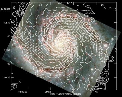
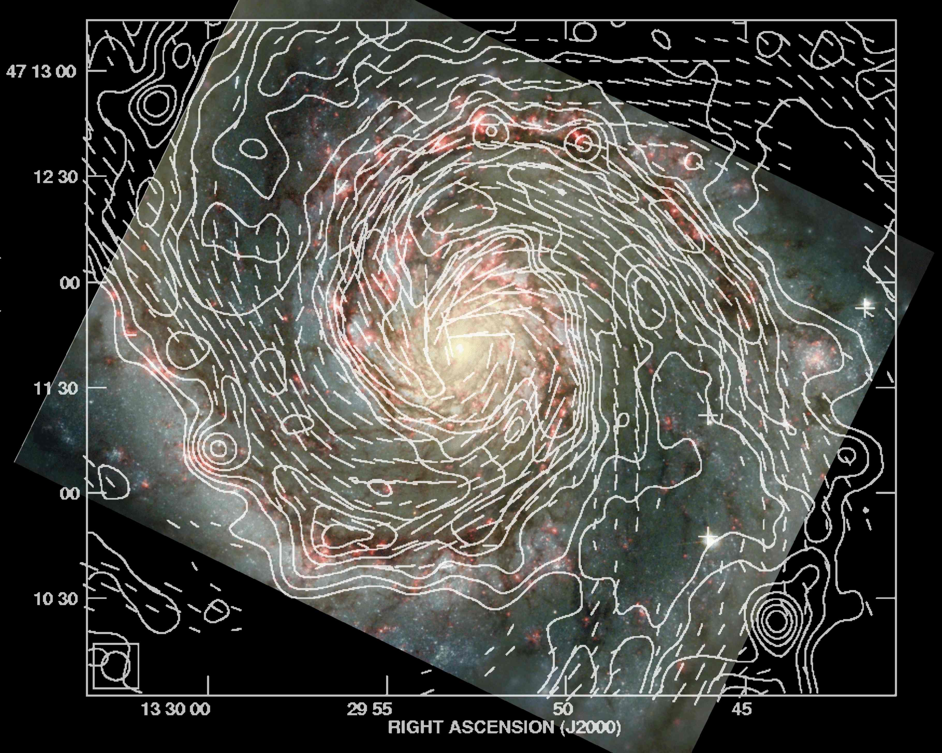
Figure 5: (a) $\lambda 3\,\mathrm{cm}$ and (b) $\lambda 6\,\mathrm{cm}$ total radio emission and $B$-vectors (VLA and Effelsberg combined) in the central $3\arcmin\times 4\arcmin$ of M51 at $8\arcsec$ resolution overlaid on a Hubble Space Telescope image (http://heritage.stsci.edu/2001/10, image credit: NASA and The Hubble Heritage Team (STScI/AURA)). Contours are at $6,12,24,36,48,96,192$ times the noise level. $B$-vectors, not corrected for Faraday rotation, are plotted where $PI\geq 3\sigma_{PI}$.

In the CO and H$\alpha$ line emissions (Fig. 4 and the red regions in Fig. 5), the spiral arms continue towards the galaxy center. The high-resolution CO map by Aalto et al. (1999) shows that the arms are sharpest and brightest between about $25\arcsec$ and $50\arcsec$ distance from the center. The arms become significantly broader and less pronounced inside a radius of about 0.8 kpc: this is inside the inner Lindblad resonance of the inner density-wave system at $r\approx 1.3\,\mathrm{kpc}$ identified by Elmegreen et al. (1989).

The polarized emission at $4\arcsec$ resolution (see Fig 6) is also strongest along the inner arms 1–2 kpc distance from the center, with typically 20% polarization. The arm–interarm contrast is at least 4 in polarized intensity (this is a lower limit as the interarm polarized emission is below the noise level at this resolution and we take $\sigma_{PI}$ as an upper limit for the interarm value), larger than that of the outer arms, and is consistent with the expectations from compression of the magnetic field in the density-wave shock (Sect. 7). The contrast weakens significantly for $r<0.8\,\mathrm{kpc}$. This may be an indication that the inner Lindblad resonance of the inner spiral density wave is at $r\simeq 0.8\,\mathrm{kpc}$ rather than $r\simeq 1.3\,\mathrm{kpc}$ (as located by Elmegreen et al. (1989)): the shock is probably weak around the inner Lindblad resonance. In total intensity, the typical arm–interarm contrast for the region of the inner arms is about 5. The actual contrast in the M51 disc alone may be stronger than this if there is significant diffuse emission in the central region from a radio halo, but this effect is hard to estimate.

In the central region, two new features appear in polarized intensity which are the brightest in the entire galaxy (Fig. 6). The first is a region $11\arcsec$ north of the nucleus with a mean fractional polarization of 10% and an almost constant polarization angle. This feature coincides with the ring-like radio cloud observed in total intensity at $\lambda 6\,\mathrm{cm}$ and at $1\arcsec$ resolution by Ford et al. (1985) who also detected polarization in this region. The polarized emission indicates that the plasma cloud expands against an external medium and compresses the gas and magnetic field. The second feature of similar intensity in polarization is a ridge located along the eastern edge of the first region, extending east of the nuclear source, with 15% mean polarization and a magnetic field almost perfectly aligned along the ridge. Field compression is apparently also strong in this ridge. The nuclear source itself appears unpolarized at this resolution.

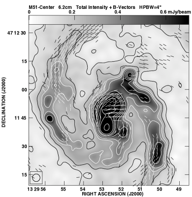
Figure 6: $\lambda 6\,\mathrm{cm}$ total radio emission (VLA and Effelsberg combined) in the central $1.4\arcmin\times 1.4\arcmin$ of M51 at $4\arcsec$ resolution. The $B$-vectors (not corrected for Faraday rotation) are shown where $PI\geq 3\sigma_{PI}$.

4 Spectral index and magnetic field strength

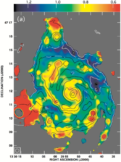
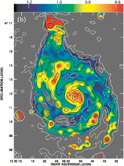
Figure 7: The spectral index maps between (a) $\lambda 20\,\mathrm{cm}$ and $\lambda 3\,\mathrm{cm}$ and (b) $\lambda 20\,\mathrm{cm}$ and $\lambda 6\,\mathrm{cm}$ at $15\arcsec$ resolution. Also shown are contours of total radio emission at $\lambda 3\,\mathrm{cm}$ (left) and $\lambda 6\,\mathrm{cm}$ (right); the contour lines are drawn at $6,12,24,36,48,96,192$ times the noise levels of $20\,\mu\mathrm{Jy/beam}$ and $30\,\mu\mathrm{Jy/beam}$ at $\lambda 3\,\mathrm{cm}$ and $\lambda 6\,\mathrm{cm}$, respectively. Spectral indices are only calculated where the signal at both wavelengths is $6$ times the noise level. The error in the fitted spectral index is typically $\pm 0.02$ in the inner galaxy and spiral arms and $\pm 0.06$ in the interarm regions at radii $\gtrsim 1\arcmin$. The large red area at the left edge of (a) is due to increased noise in the overlap region between the two VLA-pointings at $\lambda 3\,\mathrm{cm}$.

Spectral index maps of the total radio emission at $15\arcsec$ resolution are shown in Fig. 7. The spectral indices are calculated using combined Effelsberg and VLA maps that contain signal on all scales down to the beamsize. There is therefore no missing flux in these maps due to the short-spacings problem of interferometers.

Although there is good general agreement between the two spectral index maps, the spectral index between $\lambda\lambda 20,3\,\mathrm{cm}$ is generally slightly flatter than that between $\lambda\lambda 20,6\,\mathrm{cm}$; this is particularly noticeable in the spiral arms. This is due to the lower resolution of the Effelsberg $\lambda 6\,\mathrm{cm}$ map (180$\arcsec$ beam against $90\arcsec$ at $\lambda 3\,\mathrm{cm}$): $180\arcsec$ is about the radius of the M51 disc. The coarse resolution made it more difficult to fine-tune the merging of the VLA and Effelsberg data in order to match the integrated fluxes in the single-dish and merged maps. This in turn led to a slight under-representation of the single-dish data at $\lambda 6\,\mathrm{cm}$ in the merged map and thus to a slightly steeper spectral index. We believe the $\lambda\lambda 20,3\,\mathrm{cm}$ spectral index, shown in Fig. 7a, to be more reliable.

In both spectral index maps, one can clearly distinguish arms and interarm regions. The spectral index is typically in the range $-0.9\leq\alpha\leq-0.6$ in the spiral arms and $-1.2\leq\alpha\leq-0.9$ in the interarm zones. Since the spectral index in the arms is not characteristic of thermal emission ($\alpha\neq-0.1$) the arm emission must comprise a mixture of thermal and synchrotron radiation. The flatter arm spectral index can then be explained by two factors: stronger thermal emission in the arms due to recent star formation and the production of H ii regions and energy losses of cosmic ray electrons as they spread into the interarm from their acceleration sites in the arms.

We can use the observed steepening of the spectral index of the total radio emission $\alpha$ to estimate the diffusion coefficient of cosmic ray electrons in M51. We assume that the sources of the electrons are supernovae in the arms, that the initial spectral index is $\alpha_{\mathrm{syn}}\simeq-0.5$ and that the radio emission in the interarm region is predominantly synchrotron, so that $\alpha_{\mathrm{syn}}\simeq-1.1$ between the arms. A difference in the spectral indices of $\Delta\alpha=0.5$ is expected if the main mechanisms of energy losses for the electrons are synchrotron emission and inverse Compton scattering (Longair, 1994).

In the next section we estimate magnetic field strengths of around $20\,\mu\mathrm{G}$ for the inter-arm regions. In these magnetic fields, an electron emitting at $5\,\mathrm{GHz}$ has an energy of about $4\,\mathrm{GeV}$. We can estimate the lifetime of cosmic ray electrons emitting the synchrotron radiation as

$$\tau\simeq\frac{8.4\times 10^{9}}{\nu_{\mathrm{16}}^{1/2}B_{\mathrm{tot\perp}}^{3/2}}\,\mathrm{yr}\approx 8.2\times 10^{6}\,\mathrm{yr},$$

(Lang, 1999, Sect. 1.25) where the frequency $\nu_{\mathrm{16}}$ is measured in units of $16\,\mathrm{MHz}$, the total magnetic field strength in the plane of the sky $B_{\mathrm{tot\perp}}$ is measured in $\,\mu\mathrm{G}$ and we have taken $B_{\mathrm{tot\perp}}\simeq 15\,\mu\mathrm{G}$ in the interarm regions. Taking $L=1\,\mathrm{kpc}$ as the typical distance a cosmic ray electron travels from its source in a supernova remnant to the inter-arm region, yields the diffusion coefficient $D$ of the electrons,

$$D=\frac{L^{2}}{\tau}\simeq 4\times 10^{28}\,\,\mathrm{cm}^{2}\,\mathrm{s}^{-1},$$

which is compatible with the value of $D\simeq 1$–$10\times 10^{28}\,\mathrm{cm}^{2}\,\mathrm{s}^{-1}$ estimated by Strong & Moskalenko (1998) for the Milky Way. Note that cosmic ray electrons producing radio emission at cm wavelengths, propagating for a few $\,\mathrm{kpc}$ in $\,\mu\mathrm{G}$ strength magnetic fields, give diffusion coefficients in this range: our estimate for $D$ is not a unique property of the cosmic rays in M51.

4.1 Total magnetic field

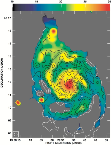
Figure 8: Total magnetic field strength, derived from the $\lambda 6\,\mathrm{cm}$ emission assuming equipartition between the energy densities of magnetic fields and cosmic rays (colour scale in $\,\mu\mathrm{G}$) along with contours of neutral gas density (a combination of CO (Helfer et al., 2003) and HI (Rots et al., 1990) observations) plotted at $1,4,8,16,32,64\%$ of the maximum value.

In order to derive the strength and distribution of the total magnetic field, we have made a crude separation of the $\lambda 6\,\mathrm{cm}$ map at $15\arcsec$ into its nonthermal $I_{\mathrm{syn}}$ and thermal $I_{\mathrm{th}}$ components. We assumed that the thermal spectral index is everywhere $\alpha_{\mathrm{th}}=-0.1$ as expected at cm wavelengths (e.g. Rohlfs & Wilson, 1999) and that the synchrotron spectral index is $\alpha_{\mathrm{syn}}=-1.1$ everywhere, as observed in the interarm regions (Fig. 7a). We are constrained in our choice of $\alpha_{\mathrm{syn}}$ by two considerations: if $\alpha_{\mathrm{syn}}>-1.1$ then thermal emission is absent from the whole inter-arm region, whereas H-$\alpha$ emission is detected; if $\alpha_{\mathrm{syn}}<-1.1$ we find that the degree of polarization approaches is maximum theoretical value of $70\%$ in many regions, which is implausible for our resolution of $570\,\mathrm{pc}$. The average thermal emission fraction at $\lambda 6\,\mathrm{cm}$ is 25%.

Assuming equipartition between the energy densities of the magnetic field and cosmic rays, a proton-to-electron ratio of 100 and a pathlength through the synchrotron-emitting regions of 1 kpc, estimates for the total field strength are shown in Fig. 8, applying the revised formulae by Beck & Krause (2005).

The strongest total magnetic fields of about $30\,\mu\mathrm{G}$ are observed in the central region of M51. The main spiral arms host total fields of 20–$25\,\mu\mathrm{G}$, while the interarm regions still reveal total fields of 15–$20\,\mu\mathrm{G}$. This is significantly larger than in spiral galaxies like NGC 6946 (Beck, 2007) and M33 (Tabatabaei et al., 2008). These two galaxies have similar star-formation rates per unit area as M51, but weaker density waves, so that compression is probably higher in M51.

4.2 Ordered magnetic field

The strength of the ordered magnetic field can be estimated from that of the total field using the degree of polarization. This method gives field strengths of $11$–$13\,\mu\mathrm{G}$ in the inner spiral arms, $8$–$10\,\mu\mathrm{G}$ in the outer spiral arms and $10$–$12\,\mu\mathrm{G}$ in the inter-arm regions. However, these values can only be attributed to a regular (or mean) magnetic field if the unresolved random component is purely isotropic (see Sokoloff et al., 1998, Sect.  5.1). The observed maximum degree of polarization of around $40\%$ can equally be produced by an anisotropic random field whose degree of anisotropy is about 2: that is if the standard deviation of the fluctuations in one direction on the plane of the sky is twice as large as in the orthogonal direction. In Sect. 6 we shall see that there is only a weak signature of a regular field in the observed multi-frequency polarization angles and that most of the polarized emission does indeed arise due to anisotropy in the random field.

The difference between the total and ordered magnetic field strengths gives an estimate for the isotropic random magnetic field strength of $18\,\mu\mathrm{G}$, or 1.5 times the ordered field, in the arms and $13\,\mu\mathrm{G}$, or 1.2 times the ordered field, in the inter-arms. If the main drivers of (isotropic) turbulence are supernova remnants, then the preferential clustering of Type II supernovae in the spiral arms is compatible with the higher fraction of isotropic random field in the arms. So a significant fraction of the magnetic field consists of a random component that is isotropic on scales less than $500\,\mathrm{pc}$.

4.3 Uncertainties

Our assumption of a synchrotron spectral index that is constant across the galaxy is crude and an oversimplification, even though the value used, $\alpha_{\mathrm{syn}}=-1.1$, can be somewhat constrained by other data as described above. We would expect that $\alpha_{\mathrm{syn}}$ should be closer to $-0.5$, the theoretical injection spectrum for electrons accelerated in supernova remnants, in parts of the spiral arms. This limitation results in an overestimate (underestimate) of the thermal (nonthermal) emission in the arms.

In principle we could combine the data at all three frequencies and simultaneously recover $I_{\mathrm{syn}}$, $I_{\mathrm{th}}$ and $\alpha_{\mathrm{syn}}$ at each pixel. However we defer a more robust calculation, interpretation and discussion to a later paper.

The equipartition estimate depends on the input parameters with a power of only $1/(3+\alpha_{\mathrm{syn}})\approx 0.24$, so that even large input errors hardly affect the results. Further errors are induced by the underestimate of the synchrotron emission in the spiral arms by the standard separation method (see above). In M33, Tabatabaei et al. (2007) found that the standard method undestimates the average nonthermal fraction by about 25%. In star-forming regions of the spiral arms, the nonthermal intensity can be a factor of two too small, which leads to an equipartition field strength which is 20% too low. In the same regions, the synchrotron spectral index is too steep by about 0.5 which overestimates the field strength by 15%. Interestingly, both effects almost cancel in M33.

The equipartition assumption itself is subject of debate. Equipartition between cosmic rays and magnetic fields likely does not hold on small spatial scales (e.g. smaller than the diffusion length of cosmic rays) and on small time scales (e.g. smaller than the diffusion time of cosmic rays).

5 Faraday rotation and depolarization

5.1 Faraday rotation

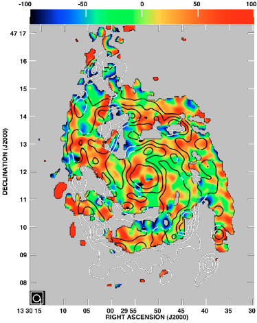
Figure 9: Rotation measures between $\lambda\lambda 3,6\,\mathrm{cm}$, at $15\arcsec$ resolution, overlaid with contours of H$\alpha$ emission (Greenawalt et al., 1998) at the same resolution, plotted at $4,8,16,32\%$ of the map maximum. Data were only used where the signal-to-noise ratio in polarized intensity exceeds three.

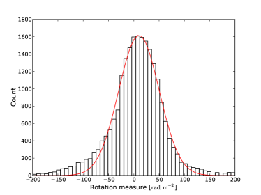
Figure 10: Distribution of rotation measures between $\lambda\lambda 3,6\,\mathrm{cm}$, shown in Fig. 9: note that the map is oversampled and so the histogram of pixel counts does not represent statistically independent data points. Data were only used where the signal-to-noise ratio in polarized intensity exceeds three. Solid line is the best-fitting Gaussian to the histogram.

The nonthermal radio emission from the arms has a relatively low degree of polarization (typically 25% at $\lambda 6\,\mathrm{cm}$ and $15\arcsec$ resolution) so that unresolved, tangled or turbulent, magnetic field dominates in the arms. In contrast, the interarm regions are up to $40\%$ polarized and host a significant fraction of magnetic fields with orientation ordered at large-scales. Whether these fields are coherent (regular) or incoherent (anisotropic turbulent) can be decided only with the help of Faraday rotation measures.

One might expect from the well-ordered, large-scale spiral patterns of the polarization vectors of Figs. 2 and 5 that the regular magnetic field would produce an obvious pattern in Faraday rotation. (See the rotation measure map of M31 in Fig. 11 of Berkhuijsen et al. (2003) for an example of clear rotation measure signal arising from a well-ordered magnetic field.) However, the Faraday rotation measure map shown in Fig. 9 is dominated by strong fluctuations in rotation measure, with a magnitude of order $100\,\mathrm{rad\,m^{-2}}$. We apparently have a paradox: the orientation of the regular magnetic field follows a systematic spiral pattern on scales exceeding $1\,\mathrm{kpc}$ but it does not produce any obvious large scale pattern in $\mathrm{RM}$. Even the magnetic arms located between the CO arms do not immediately exhibit any large-scale non-zero $\mathrm{RM}$. If the ordered field seen in polarized intensity with an equipartition strength of about $10\,\mu\mathrm{G}$ (Sect. 4) was fully regular, we would have $|\mathrm{RM}|\simeq 700\,\mathrm{rad\,m^{-2}}$ near the major axis of M51 with a systematic decrease moving away from this axis in azimuth, which is not observed (we adopt $\langle n_{\mathrm{e}}\rangle=0.1\,\mathrm{cm^{-3}}$, $h=400$ pc and an inclination of $20^{\circ}$ for this estimate, see Sect. 6.2). Note also that the overlaid H$\alpha$ contours in Fig. 9 are not generally coincident with regions of strong rotation measure.

Observational uncertainties in the measured Stokes parameters can be a source of the fluctuations in Fig. 9. The uncertainty in $\mathrm{RM}$ between $\lambda 3\,\mathrm{cm}$ and $\lambda 6\,\mathrm{cm}$, denoted here $\delta\mathrm{RM}$, depends on the signal-to-noise ratio in the polarized intensity, $\Sigma$, and the difference in the squares of the wavelengths $\delta\lambda^{2}$ as

$$\delta\mathrm{RM}=\frac{1}{\sqrt{2}\,\Sigma\,\delta\lambda^{2}}\approx\frac{280}{\Sigma}\,\mathrm{rad\,m^{-2}}.$$ (1)

Due to the steep spectral index of the synchrotron emission and the weak Faraday depolarization between $\lambda 3\,\mathrm{cm}$ and $\lambda 6\,\mathrm{cm}$, $\Sigma$ is lower at $\lambda 3\,\mathrm{cm}$ and we use these values to estimate $\delta\mathrm{RM}$. The $\mathrm{RM}$ fluctuations from the noise in the observed polarization signal are $\pm 10\,\mathrm{rad\,m^{-2}}$ (for typical $\Sigma\gtrsim 30$ in the central $r\lesssim 90\arcsec$ of Fig. 9). $\mathrm{RM}$ maps at $8\arcsec$ resolution have lower $\Sigma$ and are dominated by noise fluctuations, although some strong rotation measures, above the noise level, are also present.

The structure function of the $\mathrm{RM}$ fluctuations is flat on scales up to $3\arcmin$, whereas $\mathrm{RM}$ fluctuations due to the Milky Way foreground in the direction of M51 in the model of Sun & Reich (2009) have a slope of around $0.8$ (Reich, private communication). This is a strong indication that these fluctuations are mostly due to the magnetic field in M51.

In Fig. 9 the $\mathrm{RM}$ fluctuations with an amplitude exceeding $45\,\mathrm{rad\,m^{-2}}$, throughout the central $r\lesssim 90\arcsec$, and $55\,\mathrm{rad\,m^{-2}}$ along the outer spiral arms cannot be explained by the noise. There are therefore around ten patches where $\mathrm{RM}$ changes sign over a distance of $1$–$2\,\mathrm{kpc}$ due to intrinsic fluctuations of magnetic field.

The dispersion in $\mathrm{RM}$ is $15$–$20\,\mathrm{rad\,m^{-2}}$ measured in several regions in the inner spiral arms and $25$–$30\,\mathrm{rad\,m^{-2}}$ in the outer arms. After correction for the dispersion due to noise, the intrinsic dispersion is $11\pm 3\,\mathrm{rad\,m^{-2}}$ in the inner arms and $19\pm 5\,\mathrm{rad\,m^{-2}}$ in outer arms, hence constant within the errors. The distribution of rotation measures is shown in Fig. 10, along with the best-fit Gaussian, which has a mean $\mathrm{RM}$ of $10\pm 1\,\mathrm{rad\,m^{-2}}$ and a dispersion of $28\pm 1\,\mathrm{rad\,m^{-2}}$.

Intrinsic fluctuations dominate the $\mathrm{RM}$ maps; even smoothed to linear scales of order $1\,\mathrm{kpc}$, no large-scale pattern in rotation measure is apparent, in contrast to the clear large-scale spiral structure in polarization angles. This result is quite surprising, as we would expect to see the components of the same field in the sky plane and along the line of sight in polarization angle and in Faraday rotation, respectively. As polarization angles are not sensitive to field reversals, the observation of ordered pattern in angles does not demonstrate the existence of a regular (coherent) field. The spiral field seen in polarization angle could be anisotropic with many small-scale reversals, e.g. produced by strong shearing gas motions and compression, and hence would not contribute to Faraday rotation. Alternatively, the field may have significant components perpendicular to the galaxy plane (due to loops, outflows etc.) which are mostly visible in Faraday rotation and hide the large-scale pattern. Such an underlying large-scale pattern indeed exists, as we discuss in the next section.

The close alignment of the observed field lines along the CO arms and the lack of enhanced Faraday rotation in the polarized ridges can be understood if the turbulent magnetic field is anisotropic. An anisotropic turbulent field can produce strong polarized emission, but not Faraday rotation. This picture is similar to that obtained for the effect of large-scale shocks on magnetic fields in the barred galaxies NGC 1097 and NGC 1365 (Beck et al., 2005) and will be investigated in detail in Sect. 7.

5.1.1 The size of turbulent cells

Here we derive a new method for estimating the size of turbulent cells in the ISM of external galaxies.

The $\mathrm{RM}$ dispersion $\sigma_{\mathrm{RM,D}}$ observed within a beam of a linear diameter $D$ is related to $\sigma_{\mathrm{RM}}$ (Eq. 5) as

$$\sigma_{\mathrm{RM},D}\simeq N^{-1/2}\sigma_{\mathrm{RM}}=\sigma_{\mathrm{RM}}\frac{d}{D}\,,$$ (2)

where $N=(D/d)^{2}$ is the number of turbulent cells within the beam area, assumed to be large. We confirmed the approximate scaling of $\sigma_{\mathrm{RM},D}$ with $D^{-1}$ using $\mathrm{RM}$ maps smoothed from 8″ to 12″ where the noise fluctuations are not dominant. Combination with Eq. (5) allows us to estimate the least known quantity involved, the diameter of a turbulent cell (or twice the correlation scale of the turbulence):

$$d\!\!\! \simeq \!\!\!\left[\frac{D\sigma_{\mathrm{RM},D}}{0.81\langle n_{\mathrm{e}}\rangle B_{\mathrm{r}}(L)^{1/2}}\right]^{2/3}$$

$$= \!\!\!50\,\mathrm{pc}\left(\frac{D}{600\,\mathrm{pc}}\right)^{2/3}\left(\frac{\sigma_{\mathrm{RM},D}}{15\,\mathrm{rad\,m^{-2}}}\right)^{2/3}\left(\frac{\langle n_{\mathrm{e}}\rangle}{0.1\,\mathrm{cm}^{-3}}\right)^{-2/3}$$

$$\mbox{}\times\left(\frac{B_{\mathrm{r}}}{20\,\mu\mathrm{G}}\right)^{-2/3}\left(\frac{L}{1\,\mathrm{kpc}}\right)^{-1/3}.$$

5.2 Faraday depolarization

Faraday depolarization $\mathrm{DP}$ gives important information about the density of ionized gas, the strength of the regular and turbulent field components, and the typical length scale (or integral scale) of turbulent magnetic fields. $\mathrm{DP}$ is usually defined as the ratio of the degrees of polarization of the synchrotron emission at two wavelengths. This requires subtraction of the thermal emission which is subject to major uncertainties (see Sect. 4). Instead $\mathrm{DP}$ was computed, from the polarized intensities $P$, as $\mathrm{DP}=(PI_{1}/PI_{2})\times(\nu_{2}/\nu_{1})^{\alpha_{\mathrm{syn}}}$, where $\alpha_{\mathrm{syn}}=-1.1$ is the synchrotron spectral index, assumed to be constant across the galaxy. Variations in $\alpha_{\mathrm{syn}}$ affect $\mathrm{DP}$ less severely than errors in the estimate of the thermal fraction of the total radio emission. The $\mathrm{DP}$ maps derived for $\lambda 6\,\mathrm{cm}$ and $\lambda 3\,\mathrm{cm}$ and between $\lambda 20\,\mathrm{cm}$ and $\lambda 6\,\mathrm{cm}$ are shown in Fig. 11.

$\mathrm{DP}(6\,\mathrm{cm}/3\,\mathrm{cm})$ (Fig. 11a) is around unity (i.e. no Faraday depolarization) in most of the galaxy. Small patches with noticeable Faraday depolarization, where $\mathrm{DP}=0.6$–$0.7$ are generally found in the spiral arms. There is no systematic connection between the depolarization and the intensity of H$\alpha$ emission, indicating that variations in the thermal electron density are not the main source of the depolarization. The average value of $\mathrm{DP}(20\,\mathrm{cm}/6\,\mathrm{cm})$ (Fig. 11b) is 0.28, smaller by a factor of about 3 than $\mathrm{DP}(6\,\mathrm{cm}/3\,\mathrm{cm})$. In the inner arms, $\mathrm{DP}(20\,\mathrm{cm}/6\,\mathrm{cm})$ is lower than 0.2. Only in the outer regions of the disc does $\mathrm{DP}(20\,\mathrm{cm}/6\,\mathrm{cm})$ increase to 0.5 or higher.

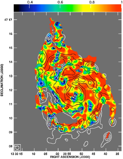
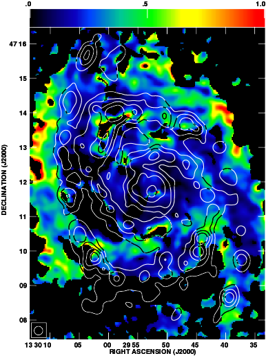
Figure 11: Depolarization between (a) $\lambda 6\,\mathrm{cm}$ and $\lambda 3\,\mathrm{cm}$ and (b) between $\lambda 20\,\mathrm{cm}$ and $\lambda 6\,\mathrm{cm}$, both at $15\arcsec$ resolution. Also shown are contours of H$\alpha$ emission (Greenawalt et al., 1998) at the same resolution, plotted at $4,8,16,32,74\%$ of the map maximum.

Differential Faraday rotation within the emitting layer leads to depolarization which varies as a $\sin(x)/x$, with $x=2\,|\mathrm{RM}_{i}|\,\lambda^{2}$, where $\mathrm{RM}_{i}$ is the intrinsic Faraday rotation measure within the emitting layer (Burn, 1966; Sokoloff et al., 1998). With typical values $|\mathrm{RM}_{i}|=50\,\mathrm{rad\,m^{-2}}$ (Fig. 9), we expect little depolarization ($\mathrm{DP}\approx 0.98$) at $\lambda 6.2\,\mathrm{cm}$ and even less at $\lambda 3.6\,\mathrm{cm}$. At $\lambda 20.5\,\mathrm{cm}$, significant $\mathrm{DP}$ is expected for $|\mathrm{RM}_{i}|>30\,\mathrm{rad\,m^{-2}}$. Furthermore, lines of zero polarization (‘canals’) are expected along level lines with $|\mathrm{RM}_{i}|=37.5n\,\mathrm{rad\,m^{-2}}$ (with integer $n\neq 0$) (Shukurov & Berkhuijsen, 2003; Fletcher & Shukurov, 2008), but not a single ‘canal’ is observed in the $\lambda 20.5\,\mathrm{cm}$ polarized intensity map. This suggests that the average $|\mathrm{RM}_{i}|$ at $\lambda 20.5\,\mathrm{cm}$ is significantly smaller than $37.5\,\mathrm{rad\,m^{-2}}$. Since the depolarization is relatively strong, it must be due to a different mechanism, e.g., Faraday dispersion.

Internal Faraday dispersion by turbulence in the magneto-ionic interstellar medium is the probable source of strong depolarization at longer wavelengths, producing the degree of polarization given by (Burn, 1966; Sokoloff et al., 1998):

$$p=p_{0}\frac{1-\exp(-2S)}{2S}\,,$$ (4)

where $S=\sigma_{\mathrm{RM}}^{2}\lambda^{4}$ and the maximum degree of polarization is $p_{0}\approx 0.7$. Here $\sigma_{\mathrm{RM}}$ is the dispersion of intrinsic rotation measure $\mathrm{RM}_{i}$ within the volume traced by the telescope beam,

$$\sigma_{\mathrm{RM}}=0.81\langle n_{\mathrm{e}}\rangle B_{\mathrm{r}}(Ld)^{1/2}\,,$$ (5)

where $\langle n_{\mathrm{e}}\rangle$ is the average thermal electron density along the line of sight (in $\,\mathrm{cm^{-3}}$), $B_{\mathrm{r}}$ the strength of the component of the random field along the line of sight (in $\,\mu\mathrm{G}$), $L$ the total path-length through the ionized gas (in pc), $d$ the size (diameter) of a turbulent cell (in pc). Reasonable values for the thermal disc of $\langle n_{\mathrm{e}}\rangle=0.1\,\mathrm{cm^{-3}}$, $L=800$ pc (estimated for $2.4<r<4.8\,\mathrm{kpc}$ by Berkhuijsen et al., 1997), $B_{\mathrm{r}}=20\,\mu\mathrm{G}$ (Sect. 4), $d=50$ pc (see Sect. 5.1) yield $\sigma_{\mathrm{RM}}\approx 300\,\mathrm{rad\,m^{-2}}$ resulting in $p/p_{0}\approx 0.002$, a very strong depolarizing effect. The resulting Faraday depolarization is $\mathrm{DP}=0.002$ between $\lambda 20.5\,\mathrm{cm}$ and $\lambda 6.2\,\mathrm{cm}$, much smaller than the observed depolarization of $\mathrm{DP}=0.2$.

We conclude that the $\lambda 20\,\mathrm{cm}$ polarized emission must originate from a layer at a greater height in the galaxy than the bulk of the $\lambda 3\,\mathrm{cm}$ and $\lambda 6\,\mathrm{cm}$ polarized emission, as the $\lambda 20\,\mathrm{cm}$ disc contribution to the polarized signal that we observe in Fig. 3 must be severely depolarized. Two possibilities, that are not mutually exclusive, are that (i) the scale height of the $\lambda 20\,\mathrm{cm}$ synchrotron disc is greater than the scale height of the thermal electron disc, or (ii) the $\lambda 20\,\mathrm{cm}$ polarized emission is produced in a synchrotron halo. In either case, since Faraday rotation is observed at wavelengths around $\lambda 20\,\mathrm{cm}$ (Horellou et al., 1992; Heald et al., 2009), with about $1/5$ the amplitude as between $\lambda 3\,\mathrm{cm}$ and $\lambda 6\,\mathrm{cm}$ (see below), thermal electrons and a magnetic field are required in the halo.

In contrast, at $\lambda 3.6\,\mathrm{cm}$ $\sigma_{\mathrm{RM}}\approx 300\,\mathrm{rad\,m^{-2}}$ produces virtually no depolarization with $p/p_{0}\approx 0.85$, so we expect that the galaxy is transparent (or Faraday thin) at $\lambda 3.6\,\mathrm{cm}$. At $\lambda 6.2\,\mathrm{cm}$ we have $p/p_{0}\approx 0.3$, moderate depolarization, with $DP=0.2$ between $\lambda 6.2\,\mathrm{cm}$ and $\lambda 3.6\,\mathrm{cm}$. This rough estimate for $DP$ is the same order of magnitude as the $DP$ shown in Fig. 11(a), albeit about three times lower than the typical observed value of $DP\approx 0.9$, indicating that our value of $\sigma_{\mathrm{RM}}$ is a slight overestimate. (The uncertainty in the adopted values of $\langle n_{\mathrm{e}}\rangle$, $L$ and $B_{\mathrm{r}}$ can easily explain the discrepancy: for $\sigma_{\mathrm{RM}}\approx 200\,\mathrm{rad\,m^{-2}}$ we have $DP=0.6$, much closer to the observed values.) Since Faraday effects are so small at $\lambda 3.6\,\mathrm{cm}$, Fig. 11(a) strongly indicates that the disc is also Faraday thin at $\lambda 6.2\,\mathrm{cm}$.

6 Regular magnetic field structure

6.1 The method

The map of Faraday rotation discussed in Sect. 5.1 clearly shows the effects of strong magnetic field fluctuations on scales of $300\,\mathrm{pc}$ to $\sim 1\,\mathrm{kpc}$; from this map one could expect the magnetic field to be rather chaotic and disordered. However, the observed polarization angles, shown in Figs. 1 and 2, suggest an underlying spiral pattern to the magnetic field on scales $\gtrsim 1\,\mathrm{kpc}$ even when corrected for Faraday rotation (Fig. 4). If the large-scale spiral pattern in the magnetic field is due to a regular field component, such as might be expected due to mean-field dynamo action, we can expect to find a signature of such a field in the Faraday rotation signal at relevant scales. If no such signal can be uncovered then we may conclude that the data do not support the presence of a mean field in M51 and that the spiral patterns seen in Figs. 1 and 2 are being imprinted on a purely random magnetic field through e.g. large-scale compression in the gas flow.

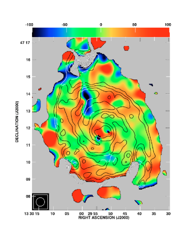
Figure 12: Rotation measures between $\lambda\lambda 3,6\,\mathrm{cm}$, at $30\arcsec$ resolution, overlaid with contours of mid-infrared 15$\,\mu$m emission (Sauvage et al., 1996) plotted at $1,2,4,8,16,32\%$ of the maximum value. Data were only used where the signal-to-noise ratio in polarized intensity exceeds five.

Figure 12 shows a Faraday rotation map using our $\lambda 3\,\mathrm{cm}$ and $\lambda 6\,\mathrm{cm}$ data smoothed to $30\arcsec$ resolution: large-scale structure in the rotation measure distribution across the disc is now visible (cf. Fig. 9). The rotation measures between $\lambda 18\,\mathrm{cm}$ and $\lambda 20\,\mathrm{cm}$ also show large-scale structure (Horellou et al., 1992, Fig. 9), but with a markedly different pattern. The complex regular magnetic field structure producing the observed rotation measure patterns cannot be reliably determined from an intuitive analysis of these maps. For example, a simple axisymmetric or bisymmetric field would produce a single or double period variation with azimuth, whereas the actual pattern is clearly more complicated. A particular difficulty is that the pattern in the observed Faraday rotation is very different between the pairs of short and long wavelengths, indicating that two Faraday-active layers may be present.

In order to look for the signature of a regular magnetic field in the multi-frequency polarization maps we applied a Fourier filter to the $15\arcsec$ resolution Stokes $Q$ and $U$ maps at $\lambda\lambda 3,6,20\,\mathrm{cm}$ to remove the signal on scales $\lesssim 30\arcsec\approx 1.1\,\mathrm{kpc}$. We also used the $\lambda 18\,\mathrm{cm}$ data of Horellou et al. (1992) which has a resolution of $43\arcsec$ resolution and was not filtered. Then maps of polarization angle were constructed at each wavelength. These were subsequently averaged in sectors with an opening angle of $20^{\circ}$ and radial ranges of $2.4-3.6\,\mathrm{kpc}$, $3.6-4.8\,\mathrm{kpc}$, $4.8-6.0\,\mathrm{kpc}$ and $6.0-7.2\,\mathrm{kpc}$ (see Fig. 14). We estimated that the minimum systematic errors in polarization angle arising from this method are about $4\degr$ at $\lambda\lambda 3,6\,\mathrm{cm}$ and $10\degr$ at $\lambda\lambda 18,20\,\mathrm{cm}$, with the main source of error being uncertainties arising from Faraday rotation by the random magnetic field (see Ruzmaikin et al., 1990, Sect. 2). We set these as minimum errors in the average polarization angles, otherwise using the standard deviation in the sector.

We applied a method that seeks to find statistically good fits to the polarization angles using a superposition of azimuthal magnetic field modes $\exp(im\phi)$ with integer $m$, where $\phi$ is the azimuthal angle in the galaxy’s plane measured anti-clockwise from the north end of the major axis. A three-dimensional model of the regular magnetic field is fitted to the observations of polarization angles at several wavelengths simultaneously. The polarization angle affected by Faraday rotation is given by $\psi=\psi_{0}+\mathrm{RM}\lambda^{2}+\mathrm{RM_{fg}}\lambda^{2}$, where the intrinsic angle of polarized emission is $\psi_{0}$, $\mathrm{RM}$ is the Faraday rotation caused by the magneto-ionic medium of M51 and $\mathrm{RM_{fg}}$ is foreground Faraday rotation arising in the Milky Way. The method of modelling is described in detail in Berkhuijsen et al. (1997) and Fletcher et al. (2004) and has been successfully applied to normal spiral galaxies (Berkhuijsen et al., 1997; Fletcher et al., 2004; Tabatabaei et al., 2008) and barred galaxies (Moss et al., 2001; Beck et al., 2005). We have derived a new model of the regular magnetic field in M51 as our combined VLA + Effelsberg maps at $\lambda\lambda 3,6\,\mathrm{cm}$ are a significant improvement in both sensitivity and resolution over the maps used by Berkhuijsen et al. (1997).

The fitted parameters of the regular magnetic fields are given in Appendix A. These fit parameters can be used to reconstruct the global magnetic structure in M51. In order to obtain statistically good fits to the observed data we needed plane-parallel field components only (no vertical fields). No satisfactory fits could be found, using various combinations of the azimuthal modes m=0, 1, 2 for the horizontal field and m=0,1 for the vertical field, for the observations at all 4 wavelengths for a single layer. Therefore at least two separate regions of Faraday rotation are required. This is because the patterns of polarization angle and Faraday rotation at $\lambda\lambda 3,6\,\mathrm{cm}$ and $\lambda\lambda 18,20\,\mathrm{cm}$ are very different: at $\lambda 18\,\mathrm{cm}$ and $\lambda 20\,\mathrm{cm}$ the disc emission is heavily depolarized by Faraday dispersion (see Sect. 5.2), so we only see polarized emission at these wavelengths from the top of the disc. A similar requirement for two Faraday rotating layers in M51 was also found by Berkhuijsen et al. (1997).

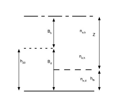
Figure 13: Geometry of the disc and halo layers. The thermal disc and halo have thickness $h_{\mathrm{th}}$ and $Z$, and electron densities $n_{{}_{\mathrm{e}},\mathrm{d}}$ and $n_{{}_{\mathrm{e}},\mathrm{h}}$. The scale-height of the region emitting polarized synchrotron radiation at $\lambda\lambda 18,20\,\mathrm{cm}$ is $h_{20}$ and the observed $\lambda 20\,\mathrm{cm}$ polarized emission comes from the layer $h_{\mathrm{th}}<z<h_{20}$, due to Faraday depolarization. The regular magnetic field has two layers: the disc $B_{\mathrm{d}}$, extending to the same height as $h_{20}$, which is both an emitting and Faraday rotating layer, and the halo $B_{\mathrm{h}}$ where only Faraday rotation occurs.

To describe the two layers in the model, the Faraday rotation from M51 is split into two components, arising from a disc and halo, $\mathrm{RM}=\xi^{(D)}\mathrm{RM}^{(D)}+\xi^{(H)}\mathrm{RM}^{(H)}$, where $\xi^{(D)}$ and $\xi^{(H)}$ are parameters that allow us to model how much of the disc and halo are visible in polarized emission at a given wavelength. We use this decomposition of the $\mathrm{RM}$ into disc and halo contributions to take into account the depolarization of the $\lambda 20\,\mathrm{cm}$ emission from the thermal disc discussed in Sect. 5.2 by setting $\xi^{(D)}=0$ and $\xi^{(H)}=1$ at $\lambda\lambda 18,20\,\mathrm{cm}$ and $\xi^{(D)}=1$ and $\xi^{(H)}=1$ at $\lambda\lambda 3,6\,\mathrm{cm}$. In other words, at $\lambda\lambda 18,20\,\mathrm{cm}$ the polarized emission is produced in a thin layer that lies above the thermal disc (see Sect. 5.2) and has the same regular magnetic field configuration that produces the $\lambda\lambda 3,6\,\mathrm{cm}$ polarized emission. The $\lambda\lambda 3,6\,\mathrm{cm}$ emission is Faraday rotated in the thermal disc and the halo whereas the $\lambda\lambda 18,20\,\mathrm{cm}$ emission is only Faraday rotated in the halo: see Fig. 13.

6.2 Results

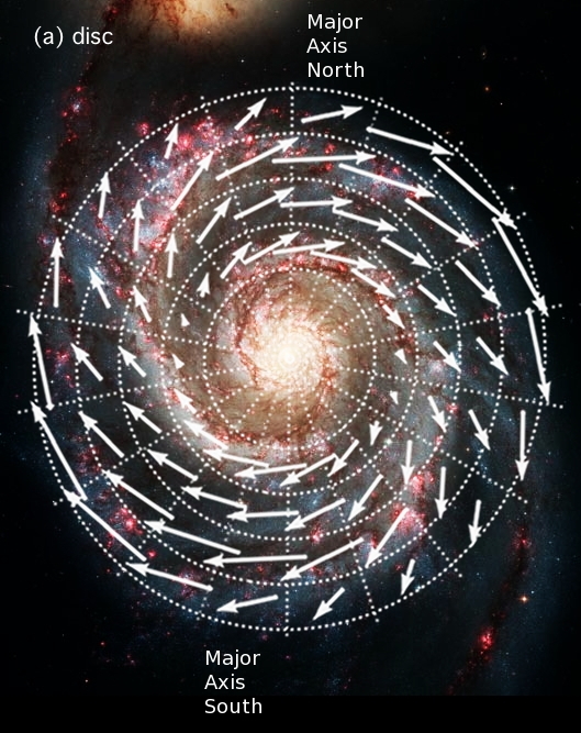
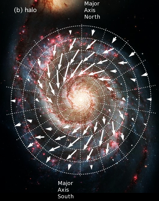
Figure 14: The regular magnetic field derived from fitting a model to the observed polarization angles at $\lambda\lambda 3,6,18,20\,\mathrm{cm}$, with the length of the magnetic field vectors proportional to the field strength, overlaid on the same optical image as in Fig. 1. (a) The regular magnetic field in the galactic disc. (b) The regular magnetic field in the galactic halo. Ring boundaries are at $2.4$, $3.6$, $4.8$, $6.0\,\mathrm{kpc}$ and $7.2\,\mathrm{kpc}$ and all sectors have an opening angle of $20^{\circ}$. The major axis is indicated: the midpoints of these two sectors correspond to $\phi=0^{\circ}$ and $\phi=180\degr$ respectively.

The resulting regular magnetic field structure is shown in Fig. 14. The regular field in the disc is best described by a superposition of m=0 and m=2 horizontal azimuthal modes and has a radial component directed outwards from the galaxy centre, whereas the halo field has a strong $m=1$ horizontal azimuthal mode and is directed inwards in the north, opposite to the direction of the disc field, and outwards in the south, same as the disc field. Oppositely directed components of the field in the disc and halo were also found by Berkhuijsen et al. (1997), however our new observations place the strong $m=1$ mode, and the resulting strong asymmetry in the magnetic field, in the halo rather than the disc. We believe that the difference in fitted fields arises from the higher quality of the new $\lambda\lambda 3,6\,\mathrm{cm}$ data, as discussed above. Heald et al. (2009) derived rotation measure maps from multi-channel WSRT data at $\lambda 22\,\mathrm{cm}$ using the RM-synthesis technique that qualitatively show the pattern expected from a $m=1$ magnetic field. Since depolarization due to Faraday dispersion cannot be removed by RM-synthesis, this gives a second, independent, indication that the halo of M51 hosts an $m=1$ regular magnetic field.

In the ring $2.4<r<3.6\,\mathrm{kpc}$ a weak $m=0$ mode is required to fit the data. This arises due to a sharp change in the observed polarization angles at $\lambda\lambda 18,20\,\mathrm{cm}$ between $\phi=120\degr$ and $\phi=140\degr$. Even with two halo modes we cannot capture the rapid change in angles and had to exclude the $\lambda 20\,\mathrm{cm}$ data at $\phi=140\degr$: the alternative would be to add an extra mode, with three new parameters, to model one data point.

The process by which two different regular magnetic field patterns in two layers of the same galaxy are produced is not clear and is beyond the scope of this paper. We only offer some speculative suggestions: (i) both fields might be generated by mean field dynamos but operating in different regimes, with the interaction of M51 with NGC 5195 driving a $m=1$ mode in the halo; (ii) the halo field could be a relic of the magnetic field present in the tenuous intergalactic medium from which the galaxy formed; (iii) as the disc field is advected into the halo it can be modified by the halo velocity field into the $m=1$ pattern. All of these possibilities will require careful modelling to determine their applicability to the problem.

In the disc of M51, in the four rings used in our model the $m=0$ azimuthal field component is $1$–$2$ times the strength of the $m=2$ mode (Table 3). While the strength of the $m=2$ mode remains approximately constant between the rings, the $m=0$ mode is of similar strength in the inner ring, but is much stronger in the other three rings.

The r.m.s. regular field strength $\bar{B}$ in each ring can be determined by integrating the fitted modes over azimuth (Table 3) via

$$\bar{B}=\frac{\bar{R}}{88\,\mathrm{rad\,m^{-2}}}\left(\frac{\langle n_{\mathrm{e,d}}\rangle}{0.11\,\mathrm{cm^{-3}}}\right)^{-1}\left(\frac{h_{\mathrm{th}}}{1\,\mathrm{kpc}}\right)^{-1}\,\,\mu\mathrm{G},$$

where

$$\bar{R}=\frac{1}{2\pi}\int^{2\pi}_{0}\sqrt{R_{r}^{2}+R_{\phi}^{2}}\,\mathrm{d}\phi$$

with $R_{r}$ and $R_{\phi}$ given by Eq. (6). Berkhuijsen et al. (1997) estimated that $\langle n_{\mathrm{e,d}}\rangle=0.11\,\mathrm{cm^{-3}}$ and $h_{\mathrm{th}}=400\,\mathrm{pc}$ in the radial range $2.4<r<4.8\,\mathrm{kpc}$ and for $4.8<r<7.2\,\mathrm{kpc}$ they estimated $\langle n_{\mathrm{e,d}}\rangle=0.06\,\mathrm{cm^{-3}}$ and $h_{\mathrm{th}}=600\,\mathrm{pc}$. The r.m.s. strengths of the large-scale magnetic field, using these parameters, are $\bar{B}=1.4\pm 0.1\,\mu\mathrm{G}$, $\bar{B}=1.7\pm 0.5\,\mu\mathrm{G}$, $\bar{B}=2.7\pm 1.0\,\mu\mathrm{G}$ and $\bar{B}=2.8\pm 0.1\,\mu\mathrm{G}$ in the rings $2.4<r<3.6\,\mathrm{kpc}$, $3.6<r<4.8\,\mathrm{kpc}$, $4.8<r<6.0\,\mathrm{kpc}$ and $6.0<r<7.2\,\mathrm{kpc}$ respectively. These are a factor of 4 lower than the strength of the ordered field derived from the equipartition assumption (Sect. 4.2). The equipartition field strength is based on the observed polarized intensity and an anisotropic random magnetic field can contribute to the polarized signal (see Sect. 4.2) but will not produce any systematic pattern in polarization angles at different frequencies. This is probably the reason for the discrepancy: most of the polarized radio emission in M51 does not trace a mean magnetic field, only the modelled large-scale pattern in Faraday rotation does.

The average pitch angle of the $m=0$ mode is $-20^{\circ}$ with little variation in radius between the rings. This means that the spiral structure of the regular field is coherent over the whole galaxy. The weaker $m=2$ modes produce an azimuthal variation in pitch angle of about $15\degr$ in the inner ring and $5\degr$ in the other rings. This variation of the pitch angle of the regular magnetic field with azimuth is much lower than the variation of the pitch angle of the ordered magnetic field observed in polarization: Patrikeev et al. (2006) showed that the orientation of Faraday rotation corrected polarization angles change by about $30\degr$. Thus the anisotropic random magnetic field, that we believe produces most of the polarized emission in M51, has a stronger azimuthal variation in its orientation: this is to be expected if the anisotropy arises from some periodic mechanism such as compression in spiral arms or localised enhanced shear.

The bisymmetric halo field has a much larger pitch angle of about $-50^{\circ}$ in the inner three rings. If this field is generated by a mean field dynamo the high pitch angles may be an indication that differential rotation in the halo is weak and an $\alpha^{2}$-dynamo action is significant. (In an $\alpha^{2}$-dynamo, shear due to differential rotation is negligible and so $|B_{r}|\approx|B_{\phi}|$.) The average thermal electron density and size of the halo in this galaxy are unknown and we have no specific constraints to apply. Taking reference values of $\langle n_{\mathrm{e,h}}\rangle=0.01\,\mathrm{cm^{-3}}$, $Z=5\,\mathrm{kpc}$ and $\langle n_{\mathrm{e,h}}\rangle=0.06\,\mathrm{cm^{-3}}$, $Z=3.3\,\mathrm{kpc}$ for the radial ranges $2.4\leq r\leq 4.8\,\mathrm{kpc}$ and $4.8\leq r\leq 7.2\,\mathrm{kpc}$ respectively, where the densities are one tenth of the disc density as in the Milky Way and $Z$ is as estimated by Berkhuijsen et al. (1997), the r.m.s. strength of the halo field (note that the $m=1$ mode means there are two values of the azimuth in each ring where the field is zero) is

$$\bar{B}\approx\frac{\bar{R}_{h}}{8\,\mathrm{rad\,m^{-2}}}\left(\frac{\langle n_{\mathrm{e,h}}\rangle}{0.01\,\mathrm{cm^{-3}}}\right)^{-1}\left(\frac{Z}{1\,\mathrm{kpc}}\right)^{-1}\,\,\mu\mathrm{G},$$

where $\bar{R_{h}}$ is the average amplitude of the halo mode. The fitted amplitudes of the halo field given in Table 3 give r.m.s. regular field strengths in the halo of $1.3\pm 0.3$, $1.2\pm 0.4$, $2.2\pm 1.0$ and $1.6\pm 0.6\,\mu\mathrm{G}$ in the four rings, with increasing radius.

We are confident that the azimuthal modes and pitch angles, fitted to our data, for the regular magnetic field in the disc and halo are robust as we have carried out extensive checks and searches of the parameter space. For example, if the $\lambda\lambda 18,20\,\mathrm{cm}$ data is ignored and a disc only model used the $\lambda\lambda 3,6\,\mathrm{cm}$ data produce a very similar fitted field to that given in Table 3. However, we cannot consider the mode amplitudes to be reliable other than to reflect the relative strengths of the $m=0$ and $m=2$ modes in the disc.

A field reversal between the regular fields in the disc and the inner halo has also been suggested in the Milky Way (Sun et al., 2008), perhaps similar to the northern half of M51 (Fig. 14).

It is probable that our model for the vertical structure of M51 (Fig. 13) is too simple and that this has lead to too much Faraday rotation being put into the halo field at the expense of the disc. In particular we do not allow for Faraday rotation from the thin emitting part of the $\lambda 20\,\mathrm{cm}$ disc nor for emission at any wavelength from the halo. Furthermore, each azimuthal mode is assumed to have an azimuth-independent intrinsic pitch angle. Adding more parameters to this model, given the limited number of sectors and frequencies that we can use, will not likely resolve this question. A more productive approach will be to develop a new model that also takes into account depolarizing effects directly and whose outputs are statistically compared directly to the individual maps, including the unpolarized emission (perhaps using the maps of Stokes parameters themselves).

7 Arm–interarm contrasts

Table 2: Arm–interarm contrasts in observed quantities. Radio intensities at $\lambda 6\,\mathrm{cm}$ are shown. The data has been smoothed to $15\arcsec$ resolution and the arm and interarm regions identified using a mask derived from the wavelet transform of the combined CO and HI map (see the text for details). The inner arm data are for a resolution of $4\arcsec$ at a position of strong contrast in polarized radio emission.

Quantity	Units	Average $1.6\,\mathrm{kpc}<r<4.8\,\mathrm{kpc}$			Inner arms $0.8\,\mathrm{kpc}<r<1.6\,\mathrm{kpc}$
		Arm	Interarm	Arm/interarm ratio	Arm	Interarm	Arm/interarm ratio
Neutral gas column density	$10^{21}\mathrm{H}\,\mathrm{cm}^{-2}$	18.0	4.0	4.5	200	40	5
Total radio intensity	$\,\mathrm{mJy/beam}$	1.1	0.5	2.2	0.6	0.12	5
Polarized radio intensity	$\,\mathrm{mJy/beam}$	0.1	0.1	1.0	0.07	$<0.01$	$\geq 7$

We wish to investigate the effect of magnetic field compression in the large-scale shocks associated with the spiral arms. In particular, how the regular and random magnetic field components are changed by the shocks and whether shock compression of isotropic random magnetic fields can produce enough anisotropic field to account for most of the polarized emission as inferred in Sections 5.2 and 6. We have carefully examined the azimuthal variations in the various maps at different radii: these emission profiles clearly demonstrate that there is not a simple azimuthal behaviour of any of the measured quantities. One cannot identify “typical” arm to interarm contrasts. So we have used a mask to separate arm (pixels in the mask set to $1$) and interarm (mask pixels set to $-1$) regions in each of the maps and hence calculate the average contrast over a wide radial range.

We combined the CO map of Helfer et al. (2003) with the HI map of Rots et al. (1990) to produce a map of the total neutral gas density at $8\arcsec$ resolution, assuming a constant conversion factor $N_{\mathrm{H}_{2}}=1.9\times 10^{20}I_{\mathrm{CO}}\,\,\mathrm{cm}^{-2}$. The arm–interarm mask was determined by making a wavelet transform, using the Mexican hat wavelet with a linear scale of about $1\,\mathrm{kpc}$, of this map. This scale was selected by examining a range of transform maps: a $1\,\mathrm{kpc}$ scale wavelet produces transform coefficients that are continuously positive along spiral arms and continuously negative in interarm regions. Also, $1\,\mathrm{kpc}$ seems reasonable as a typical width of the spiral arms in M51. This mask was used to separate the arm and interarm components of each of the maps listed in Table 2, over the radial range $1.6\,\mathrm{kpc}<r<4.8\,\mathrm{kpc}$, and then the average arm and interarm values were determined.

In addition to the data in Table 2 we also separated the rotation measures shown in Fig. 9 into arm and interarm components. We calculated the average magnitude $\left<|\mathrm{RM}|\right>$ and standard deviation $\sigma_{\mathrm{RM}}$ of $\mathrm{RM}$ and found that $\left<|\mathrm{RM}|\right>\approx 22\,\mathrm{rad\,m^{-2}}$ and $\sigma_{\mathrm{RM}}\approx 39$ in the interarm and $\left<|\mathrm{RM}|\right>\approx 15\,\mathrm{rad\,m^{-2}}$ and $\sigma_{\mathrm{RM}}\approx 29$ in the arms. This may indicate that the regular magnetic field is stronger in the interarm regions than in the arms. However, the interpretation is difficult as the $\mathrm{RM}$ distribution depends on the signal-to-noise ratio, which tends to be higher in the arms.

The contrast in the neutral gas column density (2H₂ + HI) is compatible with what might be expected from compression by a strong adiabatic shock,

$$\epsilon_{n}=n^{\mathrm{(d)}}/n^{\mathrm{(u)}}=4,$$

where the superscripts ^(d) and ^(u) refer to downstream and upstream of the shock front. We note that the scale height of the gas layer $h$ is not expected to be much affected by the spiral pattern (Shukurov, 1998); H i observations in the Milky Way suggest $h^{\mathrm{(d)}}/h^{\mathrm{(u)}}\simeq 1$–$1.5$ in the outer Milky Way (Kalberla et al., 2007).

7.1 General considerations

Explaining the arm–interarm contrast in the observed radio intensity is a long-standing problem. (Mathewson et al.1972) argued that their $\lambda 20\,\mathrm{cm}$ observations of M51 are consistent with the density wave theory of Roberts & Yuan (1970). They assumed that both cosmic ray number density and the tangential magnetic field increase in proportion to the gas density at the spiral shock. The resulting arm–interam contrast in radio intensity, after taking into account of the telescope beamwidth, is expected to be of order $10$ or more.

Tilanus et al. (1988), using observations at a higher resolution, found that the shape of cross-sectional profiles across the radio intensity arms is not compatible with the density wave theory and concluded that the synchrotron emitting interstellar medium is not compressed by shocks and decouples from the molecular clouds as it traverses the arms. Thus there is clearly a discrepancy between the physically appealing theory of Roberts & Yuan (1970) and observations (see also Condon, 1992, p. 590).

Mouschovias et al. (1974) and Mouschovias et al. (2009) suggest that only a moderate increase in synchrotron emission in spiral arms is expected due to the Parker instability: rather than being strongly compressed the regular magnetic field rises out of the disc, in loops with a scale of 500–1000 pc. However, the substantial random component of the magnetic field in M51 may supress the instability or reduce it to a simple uniform buoyancy (Kim & Ryu, 2001). Furthermore we do not observe the periodic pattern of enhanced Faraday rotation along the spiral arms that would be expected from the vertical magnetic fields at the loop footpoints (Fig. 9).

In this section we reconsider this question with additional emphasis on the polarized intensity. In Sect. 7.2, we consider how shock compression affects the emission of cosmic-ray electrons at a fixed frequency. The effect of the modest observational resolution on the arm–interarm contrasts is discussed in Sect. 7.3. In Sect. 7.4 we consider the case of compression of an isotropic random magnetic field and conclude that this may be the dominant origin of the arm–interam contrast in radio intensity only in the inner galaxy. Finally, in Sect. 7.5 we show how the decompression of an isotropic random magnetic field as it leaves the spiral arm affects the arm–interarm contrast.

7.2 Cosmic rays in compressed gas

Assuming that magnetic field is parallel to the shock front of the spiral density wave and is frozen into the gas, its strength increases in proportion to the gas density, $B\propto\rho$, as appropriate for one-dimensional compression. The ultrarelativistic gas of cosmic rays, whose speed of sound is $c/\sqrt{3}$, with $c$ the speed of light, is not compressed in the arms. However, compression of magnetic field will affect the cosmic rays (including the electron component) because $p_{\perp}^{2}/B\approx\mathrm{const}$ is an adiabatic invariant (Rybicki & Lightman, 1979), where $p_{\perp}=\gamma m_{\mathrm{e}}c$ is the component of the particle momentum perpendicular to the magnetic field and $\gamma$ is the particle Lorentz factor. More precisely, only the part of the Lorentz factor related to the particle velocity perpendicular to the magnetic field should be included, but we ignore this detail for a rough estimate. In terms of the Larmor radius $r_{B}$, one can write $p_{\perp}=eBr_{B}/c$, with $e$ the electron charge, to obtain another form of the adiabatic invariant, $Br_{B}^{2}=\mathrm{const}$, i.e. magnetic flux through the electron’s orbit remains constant. For $B\propto\rho$, we then obtain $r_{B}\propto\rho^{-1/2}$ and $p_{\perp}\propto\rho^{1/2}$, or $\gamma\propto\rho^{1/2}$.

Thus, compression of magnetic field leads to an increase in the Lorentz factor of the cosmic-ray electrons, $\gamma\propto\rho^{1/2}$. If the initial range of the Lorentz factors is $\gamma_{\mathrm{min}}^{\mathrm{(u)}}\leq\gamma\leq\gamma_{\mathrm{max}}^{\mathrm{(u)}}$, compression transforms it into $\gamma_{\mathrm{min}}^{\mathrm{(d)}}\leq\gamma\leq\gamma_{\mathrm{max}}^{\mathrm{(d)}}$ such that $\gamma_{\mathrm{min}}^{\mathrm{(d)}}/\gamma_{\mathrm{min}}^{\mathrm{(u)}}=(\rho^{\mathrm{(d)}}/\rho^{\mathrm{(u)}})^{1/2}$. Of course, the total number density of cosmic-ray particles does not change because the cosmic-ray gas is not compressed. Adopting a power-law spectrum of cosmic-ray electrons,

$$n_{\gamma}\,\,\mathrm{d}\gamma=K_{\gamma}\gamma^{-s}\,\,\mathrm{d}\gamma\;,$$

where $n_{\gamma}\,\,\mathrm{d}\gamma$ is the number of relativistic electrons per unit volume in the range $(\gamma,\gamma+\,\mathrm{d}\gamma)$, the total number density of the particles follows as $\int_{\gamma_{\mathrm{min}}}^{\gamma_{\mathrm{max}}}K_{\gamma}\gamma^{-s}\,\,\mathrm{d}\gamma\simeq\gamma_{\mathrm{min}}^{1-s}K_{\gamma}=\mathrm{const}$, where we have assumed that the energy spectrum is broad enough to have $\gamma_{\mathrm{max}}\ll\gamma_{\mathrm{min}}$ and $s>1$. However, the energy of each cosmic-ray particle increases as $\rho^{1/2}$: the energy shifts along the energy (or $\gamma$) axis, and

$$K_{\gamma}\propto\rho^{(s-1)/2}\;,$$

i.e., the number density of particles with given $\gamma$ increases with $\rho$.

Now we can estimate the effect of compression on the synchrotron emissivity observed at a fixed frequency, $\nu=\mathrm{const}$ and fixed frequency interval $\,\mathrm{d}\nu=\mathrm{const}$. Denoting $\epsilon_{I}(\nu)$ the arm–interarm contrast in $I(\nu)$ we have

$$\epsilon_{I}(\nu)=\frac{I^{(d)}}{I^{(u)}}\propto\rho^{s}\;,$$

since $I\propto K_{\gamma}B^{(s+1)/2}\propto\gamma_{\mathrm{min}}^{s-1}B^{(s+1)/2}$. Note that the Lorentz factor of the electrons which radiate at a fixed frequency $\nu\simeq\gamma^{2}B=\mathrm{const}$ reduces as $B$ increases, $\gamma(\nu)\propto B^{-1/2}$; this also leads to an increase in the number of cosmic-ray electrons radiating at a given frequency after compression since $n_{\gamma}\propto\gamma^{-s}$ and $s>0$.

With $s\simeq 3$ and the arm-interarm density contrast of about four, the number of cosmic-ray electrons with a given $\gamma$ is proportional to $K_{\gamma}\propto\rho^{(s-1)/2}\propto\rho$, and the synchrotron intensity in the spiral arms would then be 50–100 times stronger than between the arms. There are other reasons to expect enhanced synchrotron emission in the arms as supernova remnants, sites of cosmic ray acceleration, are localized in the arms. However, Table 2 clearly shows that such an enormous contrast is not observed.

It is plausible that cosmic rays are rather uniformly distributed in galactic discs and only weakly perturbed by the spiral arms (Section 3.10 of Berezinskii et al., 1990). During their lifetime within the galaxy, $\tau\simeq 3\times 10^{7}\,\mathrm{yr}$, the cosmic ray particles become well mixed over distances of order $(D\tau)^{1/2}\simeq 2$–$3\,\mathrm{kpc}$, where $D\simeq 4\times 10^{28}\,\mathrm{cm}^{2}\,\mathrm{s}^{-1}$ is the cosmic ray diffusivity. This scale exceeds the width of spiral arms, so diffusion can significantly reduce the arm-interarm contrast, but it can hardly result in the almost uniform distribution of cosmic rays which would explain the low contrasts in Table 2. Anyway, even assuming that the cosmic ray intensity is the same within the ams and between them, the compression of magnetic field by a factor of four would result in an enhancement of the synchrotron emissivity by a factor 16 for $s=3$, and this is already larger than what is observed. Note that although the contrast in total radio emission given in Table 2 includes the thermal radio emission, this is concentrated in the arms as can be seen in H$\alpha$ images (Greenawalt et al., 1998) and so the actual contrast in synchrotron emissivity will be lower than the contrast in total radio emissivity.

7.3 Telescope resolution and the width of the compressed region

One factor that can help to explain the lower than expected arm-interam contrast in total radio emission (which for simplicity we assume to be all synchrotron emission) is the possibility that the compressed region is narrow compared to the width of the spiral arms. Given the complex processes that take place as gas passes through the arms, such as the formation of molecular clouds and star formation, it is plausible that shock compression is followed by a decompression before the gas leaves the arms. Then, if the compressed region is narrower than the telescope beam the observed contrast between the arm and interarm will be reduced. We can estimate the width of the compressed region that is compatible with the observations in Table 2 using

$$\epsilon_{I}=\epsilon_{I}^{0}\frac{w}{D},$$

where $\epsilon_{I}\simeq 5$ is the observed arm-interam contrast in total radio emission in the inner spiral arms (which we assume to be all synchrotron emission to make a conservative estimate), $\epsilon_{I}^{0}\simeq 50$ is the expected contrast due to compressive effects in an adiabatic shock, $D\simeq 150\,\mathrm{pc}$ is the beamwidth at our highest resolution and $w$ is the width of the compressed region. Using the values of the parameters just quoted we obtain $w\simeq 15\,\mathrm{pc}$.

Patrikeev et al. (2006) showed that the ridge of strongest polarized emission (tracing the peak of the compressed magnetic field) is generally shifted upstream of the ridge of strongest CO emission (tracing the highest neutral gas density) in M51. We can assume that this shift is due to a spiral-shock triggering the formation of molecular clouds. The dense clouds will fill only a small fraction of the volume occupied by the ISM and may become decoupled from the magnetic field threading the diffuse ISM during their formation, as originally suggested in the case of M51 by Tilanus et al. (1988), by Beck et al. (2005) for barred galaxies and with a plausible mechanism for the separation outlined in Fletcher et al. (2009). We expect that the expansion of the compressed magnetic field will begin once the clouds have formed. Thus after a time $\tau_{c}\sim 10^{6}\,\mathrm{yr}$ the ridge in strong radio emission will begin to decay. If we estimate the magnetic field strength to be $B\simeq 20\,\mu\mathrm{G}$ (Sect. 4) then an Alfvén wave will propagate over the compressed distance $w=15\,\mathrm{pc}$ if the density, of the compressed diffuse gas in which the clouds are embedded, is $n\simeq 8\,\mathrm{cm^{-3}}$. This density is not implausible if the upstream diffuse gas density is $n\simeq 2\,\mathrm{cm^{-3}}$.

So one possible explanation for the observed low arm-interam contrast in total radio emission, compared to that expected from a simple consideration of cosmic ray energies, is that the compressed region is narrower than the beam. In this case we estimate that the ridge in compressed magnetic field, along the upstream edge of the spiral arm, will be a few tens of parsecs wide. This possibility can be tested using higher resolution observations. The cosmic rays are not the only source of the arm-interam contrast in radio emission though: next we consider the effect of a large-scale shock on the regular and random components of the magnetic field.

7.4 Compression of a partially ordered magnetic field

We consider compression of a partially ordered magnetic field by the spiral shock. We assume that the random magnetic field upstream of the shock is statistically isotropic but one-dimensional compression makes it anisotropic and so it contributes to the polarized radio emission but not to Faraday rotation. We assume that both the spiral arms and the field lines of the large-scale magnetic field are logarithmic spirals with the pitch angles $p_{\mathrm{a}}$ and $p_{b}$, respectively. An acceptable estimate is $p_{\mathrm{a}}\approx p_{b}\approx-20^{\circ}$, where negative values correspond to a trailing spiral.

The formulae required to calculate the compression of a magnetic field with both regular and isotropic random components and the associated total and polarized synchrotron emission and Faraday rotation are derived in Appendix B. Using these equations we now consider two cases that encompass the range of observed contrasts in polarized emission in M51: the inner spiral arms, where there is a strong arm–interarm contrast in polarization of at least $\epsilon_{PI}\sim 4$, and the average contrast of $\epsilon_{PI}\sim 1$ which is more representative of the greater radii. The upstream ratio of random to regular magnetic field strength $b/B$ and the increase in gas density $\epsilon_{n}=4$, in regular field $\epsilon_{B}$ and in random field $\epsilon_{b}$ fields due to the shock are fixed and then the consequential increases in nonthermal $\epsilon_{I}$ and polarized $\epsilon_{PI}$ emission across the shock are calculated.

Firstly the inner arms. Here we can obtain a reasonable match with the maximum observed arm–interarm contrasts $\epsilon_{I}\simeq 5$ (assumed to be mostly synchrotron emission) and $\epsilon_{PI}\simeq 7$ (a lower limit due to weak interarm intensity at $4\arcsec$ resolution). With the parameters $\epsilon_{B}=1$, i.e. the regular field is not increased by the shock — this can be justified, for example, if the regular magnetic field becomes detached from dense clouds as they form (Beck et al., 2005) — and $\epsilon_{b}=2.7$ we obtain expected arm–interarm contrasts in synchrotron emission of $3.3$ and polarized emission of $4.8$. If $\epsilon_{B}>1$ then the expected increase in polarization becomes much larger. For example, for $\epsilon_{B}=\epsilon_{b}=2.7$ we obtain $\epsilon_{PI}=11$: since we only have a lower limit on the observed $\epsilon_{PI}$ we cannot rule out this possibility. We conclude that in the innermost spiral arms ($r<1.6\,\mathrm{kpc}$) anisotropic random magnetic fields produced by compression of the interstellar gas in the spiral arms can account for the observed increases in total and polarized radio emission.

Now for the average arm–interarm contrasts. Here, since the average contrast in polarization is $\epsilon_{PI}\simeq 1$, this requires no increase in regular magnetic field in the arm and also no anisotropy of the random magnetic field, but simultaneously we require a small increase in synchrotron emission $\epsilon_{I}=2.2$. This is not possible in our model; it is also unlikely to happen when galaxies contain strong spiral density waves. The closest we can come is to set $\epsilon_{B}=1$ coupled with a weak upstream random field $b^{2}/B^{2}=0.2$ and strong compression of the random field $\epsilon_{b}=4.5$ to produce the required contrast in total emission. Then we can obtain arm–interarm contrasts of $2.3$ in total synchrotron emission and $1.7$ in polarization. However, $b^{2}/B^{2}=0.2$ is strongly contradicted by the equipartition estimates of the various field strengths in Sect. 4, which likely overestimate the strength of the regular field as discussed in Sect. 5.2 and 6.

To summarise this subsection: enhancement of the regular and random magnetic field components parallel to a large-scale spiral shock can partly account for the observed arm-interam contrasts in radio emission but no single set of parameters is compatible with the full range of the observations.

7.5 Decompression of an isotropic magnetic field

Finally, we consider the decompression of an isotropic field as the magnetized gas flows from a high density to a low density region. This decompression also leads to the generation of an anisotropic random magnetic field, as the field component parallel to lines of constant density increases while the perpendicular component is unaffected, similar to the compressive case. But decompression will also help to lower the arm-interam contrast in nonthermal emission, thus alleviating one of the difficulties encountered in the previous subsection, if the random field in the arms is (partly) isotropized: this can readily occur due to turbulence being driven by star formation activity and the expansion of supernova remnants.

First consider the case of straightforward compression. Let us define the $x$-direction as perpendicular to the shock and the $y$-direction as parallel: so only $y$-components of the magnetic field are affected by the shock. Thus

$$\langle b_{x}^{2(d)}\rangle=\langle b_{x}^{2(u)}\rangle=\frac{1}{3}b^{2(u)},$$

and

$$\langle b_{y}^{2(d)}\rangle=\epsilon_{\rho}^{2}\langle b_{y}^{2(u)}\rangle=\frac{1}{3}\epsilon_{\rho}^{2}b^{2(u)},$$

where $(u)$ and $(d)$ refer to upstream and downstream and $\vec{b}$ is the total random field. Now the plane-of-sky component of the random field is $b_{\perp}^{2}=b_{x}^{2}+b_{y}^{2}$ so we obtain

$$\frac{b_{\perp}^{2}(d)}{b_{\perp}^{2}(u)}=\frac{1}{2}(1+\epsilon_{\rho}^{2})\simeq 8,$$

for an adiabatic shock, where $\epsilon_{\rho}=4$. So we expect adiabatic compression in a simple, plane parallel shock to produce a contrast in nonthermal emission $\epsilon_{I}\simeq 8$, in the case that the cosmic rays are smoothly distributed. This is a simplified version of part of the calculation described above and in detail in Appendix B.

Now consider the case of decompression. We follow a similar calculation but here

$$\langle b_{y}^{2(d)}\rangle=\frac{1}{\epsilon_{\rho}^{2}}\langle b_{y}^{2(u)}\rangle=\frac{1}{3\epsilon_{\rho}^{2}}b^{2(u)},$$

which leads to

$$\frac{b_{\perp}^{2}(d)}{b_{\perp}^{2}(u)}=\frac{1}{2}(1+\frac{1}{\epsilon_{\rho}^{2}})\simeq\frac{1}{2}.$$

In this case the arm is the upstream region so the expected arm-interam contrast in nonthermal emission is $\epsilon_{I}\simeq 2$ which is close to the average contrast observed (Table 2).

7.6 Summary: compression and arm-interarm contrasts

In Sect. 5.2 and 6 we have shown that much of the polarized emission detected across the disc of M51 must come from anisotropic random fields. Combined with the problem described in Sect. 7.4 above, of how isotropic random fields can be compressed in a spiral shock but not produce an increase in polarized emission, we are led to the view that anisotropic random fields are already present in interarm regions, perhaps as a result of enhanced localised shear or decompression. Patrikeev et al. (2006) showed that the orientation of the magnetic field in M51 varies in azimuth by $\pm 15\degr$ and in the interarm generally has a different pitch angle to the CO spiral arm, only becoming well aligned with the CO arm at its location. In this case compression of the already anisotropic field in the spiral shock will only weakly amplify the random field and hence lead to a weak change in polarized emission.

We conclude that the roughly constant average polarized emission across the arms and interam region cannot be easily explained with simple models of shock compression of magnetic field, if one simultaneously considers the weak contrasts that are observed in the total emission. The arm-interarm contrast in the radio emission probably results from a complex interplay of compression and decompression of the dominant random field, occurring as the ISM undergoes phase changes on its passage through the arms. In addition the thickness of the compressed regions compared to the width of the beam likely plays a role.

8 Summary and Conclusions

• Polarized emission ($PI$) is present throughout most of the disc of M51. In some regions the strongest $PI$ coincides with the location of the strong spiral arms as seen in CO emission. In other regions $PI$ is concentrated in the interarm region, forming structures up to $\sim 5\,\mathrm{kpc}$ in size, reminiscent of the $\sim 10\,\mathrm{kpc}$-scale magnetic arms observed in NGC 6946 (Beck & Hoernes, 1996). The origin of these magnetic arms is still unknown.

• The observed polarization angles trace spiral patterns with pitch angles similar to, but not always the same as, the gaseous spiral arms. The apparently ordered large-scale magnetic field responsible for the well aligned polarization angles does not produce a systematic pattern in Faraday rotation, leading us to conclude that a large fraction of the polarized emission is caused by anisotropic small-scale magnetic fields (where small-scale refers to sizes smaller than the beam, typically $300$–$600\,\mathrm{pc}$): anisotropic random fields, whose anisotropy is caused by a large scale process (for example, compression and/or shear) and so is aligned over large distances, can produce well ordered polarization angles but a random Faraday rotation distribution.

• Faraday depolarization, caused by Faraday dispersion due to turbulent magnetic fields, leads to strong depolarization of the $\lambda 20\,\mathrm{cm}$ polarized emission from the disc. From the observed fluctuations in Faraday depolarization we were able to estimate a typical diameter of a turbulent cell as $\sim 50\,\mathrm{pc}$.

• Fourier filtering followed by averaging in sectors is necessary to reveal the contribution of the regular (or mean) magnetic field to the observed polarization signal. This allowed us to fit a model of the 3D regular magnetic field of M51 to the observations of polarization angles at $\lambda\lambda 3,6,18,20\,\mathrm{cm}$. Due to the strong depolarization at $\lambda\lambda 18,20\,\mathrm{cm}$ we were able to identify two different regular magnetic field patterns. In the thermal disc the regular field can be described as a combination of $m=0+2$ azimuthal modes, with the $m=0$ mode being the strongest: this combination can be the result of the strong two-armed spiral pattern modifying a dynamo generated $m=0$ mode (the easiest to excite according to mean-field galactic dynamo theory). The pitch angle of the $m=0$ mode is similar at all radii. In the halo the observed polarization angles at $\lambda\lambda 18,20\,\mathrm{cm}$, whose emission from the thermal disc is heavily depolarized, reveal a $m=1$ azimuthal geometry for the regular magnetic field. The origin of this halo field is unclear.

• The arm–interarm contrast in gas density and radio emission was compared to a model where a regular and (isotropic) random magnetic field is compressed by shocks along the spiral arms. We found that where a strong arm–interarm contrast in $PI$ is observed, in the inner arms $r\lesssim 1.6\,\mathrm{kpc}$, amplification of the random magnetic field by compression can successfully explain the data, provided that the regular magnetic field is not significantly increased. This constraint is similar to that obtained for two barred galaxies in Beck et al. (2005), where it was proposed that the regular magnetic field de-couples from molecular clouds as they rotate and collapse. We were unable to explain the average arm–interarm contrast in total and polarized radio emission, typical for much of the galaxy at $r>2\,\mathrm{kpc}$, by a model involving shock compression of magnetic fields. Even when the regular magnetic field is not compressed some increase in $PI$ in the arms is expected from compression of the random field, whereas the average arm–interarm contrast in $PI$ is about one: this problem could be resolved if the random field is isotropic in the arms and becomes anisotropic due to decompression as it enters the interam. Alternatively, the compressed region of magnetic field may be sufficiently narrow (with a width of about $20\,\mathrm{pc}$), as might occur if the molecular clouds are de-coupled from the synchrotron emitting gas, to reduce the arm–interarm contrast by the required degree.

Appendix A Parameters of the fitted regular magnetic fields

In Table 3 we give the parameters of the fitted regular magnetic field models discussed in Section 6. Although a component of the regular field perpendicular to the disc plane ($R_{z}$ in Eq. (6)) is allowed in the model and we searched for fits using this component, a vertical field was not required to obtain a good fit in either ring. The greater of the standard deviation and the noise within a sector was taken as the error in polarization angle.

The regular magnetic field is modelled as

$$R_{r} = R_{0}\sin p_{0}+R_{1}\sin p_{1}\cos(\phi-\beta_{1})$$

$$+\,R_{2}\sin p_{2}\cos(2\phi-\beta_{2}),$$

$$R_{\phi} = R_{0}\cos p_{0}+R_{1}\cos p_{1}\cos(\phi-\beta_{1})$$ (6)

$$+\,R_{2}\cos p_{2}\cos(2\phi-\beta_{2}),$$

$$R_{z} = R_{z0}+R_{z1}\cos(\phi-\beta_{z1})+R_{z2}\cos(2\phi-\beta_{z2}),$$

$$R_{hr} = R_{h0}\sin p_{h0}+R_{h1}\sin p_{h1}\cos(\phi-\beta_{h1}),$$

$$R_{h\phi} = R_{h0}\cos p_{h0}+R_{h1}\cos p_{h1}\cos(\phi-\beta_{h1}),$$

where $R_{i}$ is the amplitude of the $i$’th mode in units of $\,\mathrm{rad\,m^{-2}}$, $p_{i}$ is its pitch angle, $\beta_{i}$ ($i\geq 1$) determines the azimuth where the corresponding non-axisymmetric mode is maximum and the subscript _h denotes the components of the halo field. The magnetic field in each mode of this model is approximated by a logarithmic spiral, $p_{i}=\mbox{const}$, within a given ring. However, the superposition of such modes with different pitch angles leads to deviations from a logarithmic spiral. For further details of the method, see Berkhuijsen et al. (1997) and Fletcher et al. (2004).

The foreground Faraday rotation due to the magnetic field of the Milky Way $R_{\mathrm{fg}}$ was also included in the fitting; we expect $R_{\mathrm{fg}}$ to be the same in all rings and this provides a useful consistency check to the results of independent fits to the four rings. A logarithmic spiral pattern has the same pitch angle in all rings. $S$ is the residual of the fit and $S_{\lambda}$ the residual at a given wavelength. The appropriate $\chi^{2}$ value, at the $95$% confidence level, is shown for the number of fit parameters and data points. A fit is statistically acceptable if $S\leq\chi^{2}$ and the Fisher criteria, that tests if $S$ is unduly influenced by a good fit to a single wavelength, is satisfied. The $\chi^{2}$ values vary from ring to ring (even when the same number of fit parameters are used) as some sectors are excluded from the model, either because the noise in the sector exceeds the standard deviation of the measurements or because the sector represents an outlier from the global pattern.

In Figs. 15, 16, 17 and 18 we show the observed sector-averaged polarization angles and the fitted model for each ring. The fit quality is excellent at $\lambda 3\,\mathrm{cm}$ and $\lambda 6\,\mathrm{cm}$ for all rings, but in the inner two rings sharp discontinuities in the $\lambda 20\,\mathrm{cm}$ polarization angles around $\theta\simeq 120\degr$ cannot be accommodated by the model. Since the parameters of the fitted halo field are largely determined by the data at the longer wavelengths we are therefore less satisfied with the parameters of the fitted halo field in these rings than with those of the disc field, as we discuss in Sect. 6.

Table 3: Parameters of fitted model for M51, with notation as in Eq. 6. The index $h$ refers to the “halo” field. The residuals at the wavelengths $\lambda\lambda 3,6,18,20\,\mathrm{cm}$ are given in brackets.

		$2.4<r<3.6\,\mathrm{kpc}$	$3.6<r<4.8\,\mathrm{kpc}$	$4.8<r<6.0\,\mathrm{kpc}$	$6.0<r<7.2\,\mathrm{kpc}$
$R_{\mathrm{fg}}$	$\,\mathrm{rad\,m^{-2}}$	$4$ $\pm 2$	$5$ $\pm 4$	$2$ $\pm 5$	$4$ $\pm 1$
$R_{0}$	$\,\mathrm{rad\,m^{-2}}$	$-46$ $\pm 3$	$-57$ ${}^{+11}_{-20}$	$-76$ ${}^{+14}_{-27}$	$-76$ $\pm 2$
$p_{0}$	deg	$-20$ $\pm 1$	$-24$ $\pm 4$	$-22$ $\pm 4$	$-18$ $\pm 1$
$R_{2}$	$\,\mathrm{rad\,m^{-2}}$	$-33$ $\pm 2$	$-25$ ${}^{+7}_{-5}$	$-40$ ${}^{+11}_{-9}$	$-44$ $\pm 2$
$p_{2}$	deg	$-12$ $\pm 2$	$16$ ${}^{+23}_{-15}$	$8$ ${}^{+18}_{-12}$	$3$ $\pm 2$
$\beta_{2}$	deg	$-8$ $\pm 5$	$-6$ $\pm 9$	$-14$ $\pm 10$	$-25$ $\pm 2$
$R_{h0}$	$\,\mathrm{rad\,m^{-2}}$	$23$ $\pm 6$
$p_{h0}$	deg	$-43$ $\pm 13$
$R_{h1}$	$\,\mathrm{rad\,m^{-2}}$	$76$ $\pm 11$	$77$ $\pm 26$	$57$ $\pm 26$	$43$ $\pm 14$
$p_{h1}$	deg	$-45$ $\pm 5$	$-49$ $\pm 12$	$-50$ ${}^{+29}_{-23}$	$-90$ $\pm 3$
$\beta_{h1}$	deg	$44$ $\pm 5$	$30$ $\pm 14$	$-3$ ${}^{+23}_{-29}$	$-16$ $\pm 3$
$S_{\lambda}$	($\lambda\lambda 3,6,18,20\,\mathrm{cm}$)	$(14,21,21,21)$	$(9,9,20,28)$	$(10,18,11,16)$	$(10,26,21,21)$
$S$		$77$	$66$	$55$	$78$
$\chi^{2}$		$79$	$83$	$83$	$79$

One data point excluded in the ring $2.4<r<3.6\,\mathrm{kpc}$ at: $\lambda 20\,\mathrm{cm}$, $\phi=140\degr$.
Three data points excluded in the ring $6.0<r<7.2\,\mathrm{kpc}$ at: $\lambda 3\,\mathrm{cm}$, $\phi=20\degr$; $\lambda 18\,\mathrm{cm}$, $\phi=220\degr$; $\lambda 20\,\mathrm{cm}$, $\phi=180\degr$.

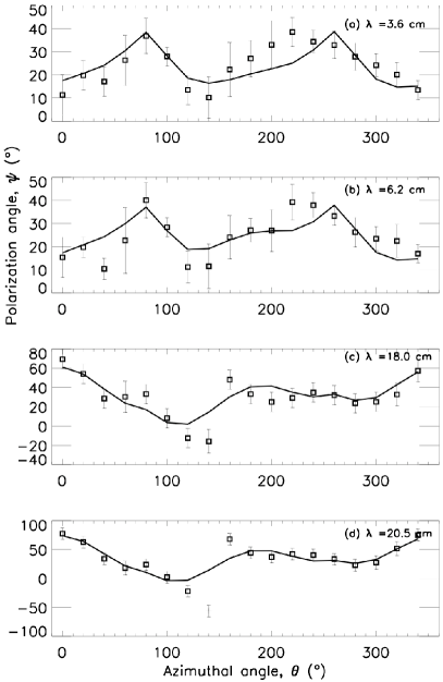
Figure 15: Polarization angles ($\psi$, measured from the local radial direction in the plane of M 51) against azimuth in the galaxy plane ($\theta$) for the ring 2.4–3.6$\,\mathrm{kpc}$. Fit (solid line) and observations (squares with error bars, horizontal lines with error bars show data points excluded from the fit) are shown for $\lambda 3\,\mathrm{cm}$, $\lambda 6\,\mathrm{cm}$, $\lambda 18\,\mathrm{cm}$ and $\lambda 20\,\mathrm{cm}$ from top to bottom. The error bars show the $1\sigma$ deviations.

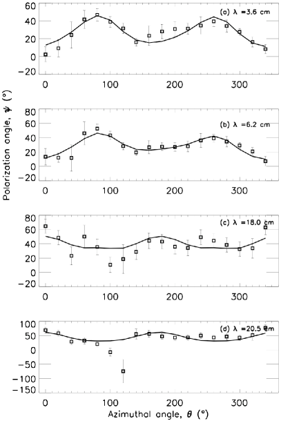
Figure 16: As in Fig. 15 but for the ring 3.6–4.8$\,\mathrm{kpc}$.

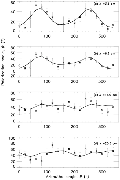
Figure 17: As in Fig. 15 but for the ring 4.8–6.0$\,\mathrm{kpc}$.

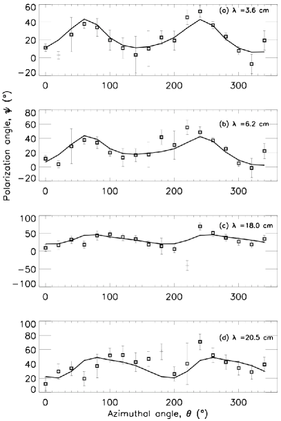
Figure 18: As in Fig. 15 but for the ring 6.0–7.2$\,\mathrm{kpc}$.

Appendix B Compression of a partially ordered magnetic field in a spiral arm

We introduce a Cartesian frame in the sky plane $(\tilde{x},\tilde{y},\tilde{z})$ centered at the galaxy center with the $\tilde{x}$-axis directed towards the western end of the major axis and the $\tilde{y}$-axis, in the northern direction; the $\tilde{z}$-axis is the directed towards the observer (and in the general direction of the galaxy’s north pole). We also introduce galaxy’s Cartesian frame $(x,y,z)$ where the $x$- and $\tilde{x}$-axes coincide and the $z$-axis is also directed towards the galaxy’s north pole. Magnetic field components in the two frames are related by (Berkhuijsen et al., 1997):

$$B_{\tilde{x}} = B_{x},$$

$$B_{\tilde{y}} = B_{y}\cos i+B_{z}\sin i,$$ (7)

$$B_{\tilde{z}} = -B_{y}\sin i+B_{z}\cos i,$$

where $i$ is the galaxy’s inclination angle, and we include $B_{z}$ for the future convenience (we recall that we can adopt $B_{z}=0$ in M51). The galaxy’s cylindrical frame $r,\phi,z$ then has the azimuthal angle measured counterclockwise (along the galaxy’s rotation) from the $x$-axis. And finally, we introduce a local Cartesian frame of the spiral shock $(x^{\prime},y^{\prime},z^{\prime})$, with the $x^{\prime}$-axis perpendicular to the shock and directed from the interarm region into the spiral arm, the $y^{\prime}$-axis parallel to the shock, so that the $z^{\prime}$-axis complements them to a right-handed triad i.e., is directed towards the north pole of the galaxy. Then the angle between the $x^{\prime}$- and $x$-axes is

$$\theta=\phi-p_{\mathrm{a}}.$$ (8)

It is convenient to specify the upstream large-scale magnetic field in the galaxy’s cylindrical frame $\vec{B}=B(\sin p_{B},\cos p_{B},0)$, where we neglect the vertical field component (see Sect. 6). Then the unit normal to the shock, in the galaxy’s frame is given by $\widehat{\vec{n}}=\widehat{\vec{x}^{\prime}}=(\cos\theta,\sin\theta,0)$, the tangent vector is given by $\widehat{\vec{t}}=\widehat{\vec{y}^{\prime}}=(-\sin\theta,\cos\theta,0)$, and the regular magnetic field components normal and tangent to the shock then follow, respectively, as

$$B_{x^{\prime}}=B\sin(p_{b}-p_{\mathrm{a}}),\quad B_{y^{\prime}}=B\cos(p_{b}-p_{\mathrm{a}}).$$

It is now easy to see that the compressed large-scale magnetic field in the spiral arm has the components

$$B^{\mathrm{(d)}}_{x^{\prime}}=B^{\mathrm{(u)}}_{x^{\prime}},\quad B^{\mathrm{(d)}}_{y^{\prime}}=\epsilon_{n}B^{\mathrm{(u)}}_{y^{\prime}},$$

where $\epsilon_{n}=n^{\mathrm{(d)}}/n^{\mathrm{(u)}}$ is the gas density compression ratio. Now we can transform both the original and compressed fields to the galaxy’s frame by rotating it by the angle $-\theta$, $B_{x}=B_{x^{\prime}}\cos\theta-B_{y^{\prime}}\sin\theta,$ $B_{y}=B_{x^{\prime}}\sin\theta+B_{y^{\prime}}\cos\theta,$ $B_{z}=B_{z^{\prime}},$ and then to the sky frame using Eq. (7), where the $\tilde{x}$ and $\tilde{y}$ component contribute to the magnetic field in the plane of the sky and $B_{\tilde{z}}$ is directed along the line of sight:

$$\vec{B}_{\perp}=(B_{\tilde{x}},B_{\tilde{y}}),\quad B_{\parallel}=B_{\tilde{z}}.$$

Similar relations can be written for the random magnetic field $\vec{b}$, but now we cannot neglect the $z$-component of the random magnetic field in the galaxy frame. The compressed random field in the shock frame is given by

$$\vec{b}^{\mathrm{(d)}}=(b^{\mathrm{(u)}}_{x^{\prime}},\epsilon_{n}b^{\mathrm{(u)}}_{y^{\prime}},\epsilon_{n}b^{\mathrm{(u)}}_{z^{\prime}})$$

which can be transformed to the galaxy’s frame and then to the sky frame to obtain

$$b_{\tilde{x}} = b_{x}=b_{x^{\prime}}\cos\theta-\epsilon_{n}b_{y^{\prime}}\sin\theta,$$

$$b_{\tilde{y}} = b_{x^{\prime}}\sin\theta\cos i+\epsilon_{n}b_{y^{\prime}}\cos\theta\cos i+\epsilon_{n}b_{z^{\prime}}\sin i,$$

$$b_{\tilde{z}} = -b_{x^{\prime}}\sin\theta\sin i-\epsilon_{n}b_{y^{\prime}}\cos\theta\sin i+\epsilon_{n}b_{z^{\prime}}\cos i.$$

Averaging using these equations then yields

$$\langle{b_{\tilde{x}}^{2}}\rangle^{\mathrm{(d)}} = \frac{1}{3}{\sigma_{b}^{2}}^{\mathrm{(u)}}\left[1+(\epsilon_{n}^{2}-1)\sin^{2}\theta\right],$$

$$\langle b_{\tilde{y}}^{2}\rangle^{\mathrm{(d)}} = \frac{1}{3}{\sigma_{b}^{2}}^{\mathrm{(u)}}\left[1+(\epsilon_{n}^{2}-1)(-1\sin^{2}\theta\cos^{2}i)\right],$$

$$\langle b_{\tilde{z}}^{2}\rangle^{\mathrm{(d)}} = \frac{1}{3}{\sigma_{b}^{2}}^{\mathrm{(u)}}\left[1+(\epsilon_{n}^{2}-1)(-1\sin^{2}\theta\sin^{2}i)\right],$$

where $\langle{b_{x^{\prime}}^{2}}\rangle^{\mathrm{(u)}}=\langle{b_{y^{\prime}}^{2}}\rangle^{\mathrm{(u)}}=\langle{b_{z^{\prime}}^{2}}\rangle^{\mathrm{(u)}}=\frac{1}{3}{\sigma_{b}^{2}}^{\mathrm{(u)}}$ (isotropy of the upstream random magnetic field), and $\langle b_{x^{\prime}}b_{y^{\prime}}\rangle^{\mathrm{(u)}}=\langle b_{x^{\prime}}b_{z^{\prime}}\rangle^{\mathrm{(u)}}=\langle b_{y^{\prime}}b_{z^{\prime}}\rangle^{\mathrm{(u)}}=0$ (statistical independence of the upstream field components).

Now the arm–interarm contrasts in various observables can be estimated as follows. For the total synchrotron intensity,

$$\epsilon_{I}\simeq\frac{{B_{\perp}^{2}}^{\mathrm{(d)}}+\langle b_{\perp}^{2}\rangle^{\mathrm{(d)}}}{{B_{\perp}^{2}}^{\mathrm{(u)}}+\langle b_{\perp}^{2}\rangle^{\mathrm{(u)}}}\,\frac{L_{I}^{\mathrm{(d)}}}{L_{I}^{\mathrm{(u)}}}\frac{n^{\mathrm{(d)}}_{\gamma}}{n^{\mathrm{(u)}}_{\gamma}},$$

where $L_{I}$ is the pathlength through the synchrotron layer and $n_{\gamma}$ the cosmic ray number density. The polarized emissivity in a partially ordered, anisotropic random magnetic field and uniform cosmic ray distribution can be calculated using Eq. (20) of Sokoloff et al. (1998) as

$$PI\propto(B_{\tilde{x}}^{2}-B_{\tilde{y}}^{2}+\langle b_{\tilde{x}}^{2}\rangle-\langle b_{\tilde{y}}^{2}\rangle)^{2}+4B_{\tilde{x}}^{2}B_{\tilde{y}}^{2}.$$

Applying this formula to the downstream magnetic field, we obtain the contrast in polarized intensity $\epsilon_{PI}$ by dividing it by $PI^{\mathrm{(u)}}\propto{B_{\perp}^{2}}^{\mathrm{(u)}}$, and also multiplying by the ratio of pathlengths $L_{I}^{\mathrm{(d)}}/L_{I}^{\mathrm{(u)}}$ and cosmic ray densities $n^{\mathrm{(d)}}_{\gamma}/n^{\mathrm{(u)}}_{\gamma}$.

The Faraday rotation measure can be calculated as $\mathrm{RM}\simeq 0.81n_{\mathrm{e}}B_{\tilde{z}}L_{\mathrm{RM}}$, where $L_{\mathrm{RM}}$ is an appropriate pathlength, and its standard deviation is obtained using Eq. (5), and then the arm–interarm contrast is calculated straightforwardly.

References

- Aalto et al. (1999) Aalto, S., Hüttemeister, S., Scoville, N. Z., & Thaddeus, P. 1999, ApJ, 522, 165
- Beck (2007) Beck, R. 2007, A&A, 470, 539
- Beck & Hoernes (1996) Beck, R., & Hoernes, P. 1996, Nat, 379, 47
- Beck & Krause (2005) Beck, R., & Krause, M. 2005, AN, 326, 414
- Beck et al. (2005) Beck, R., Fletcher, A., Shukurov, A., et al. 2005, A&A, 444, 739
- Berezinskii et al. (1990) Berezinskii, V. S., Bulanov, S. V., Dogiel, V. A., Ginzburg, V. L., & Ptuskin, V. S. 1990, Astrophysics of Comsic Rays, Amsterdam.
- Berkhuijsen et al. (1997) Berkhuijsen, E. M., Horellou, C., Krause, M., et al. 1997, A&A, 318, 700
- Berkhuijsen et al. (2003) Berkhuijsen, E. M., Beck, R., & Hoernes, P. 2003, A&A, 398, 937
- Burn (1966) Burn B. J., 1966, MNRAS, 133, 67
- Ciardullo et al. (2002) Ciardullo, R., Feldmeier, J. J., Jacoby, G. H., et al. 2002, ApJ, 577, 31
- Condon (1992) Condon, J. J. 1992, ARA&A, 30, 575
- Elmegreen et al. (1989) Elmegreen, B.G., Elmegreen, D. M., & Seiden, P. E. 1989, ApJ, 343, 602
- Emerson & Gräve (1988) Emerson, D. T., & Gräve, R. 1988, A&A, 190, 353
- Fletcher et al. (2004) Fletcher, A., Berkhuijsen, E. M., Beck, R., & Shukurov, A. 2004, A&A, 414, 53
- Fletcher & Shukurov (2008) Fletcher, A. & Shukurov, A. 2008, MNRAS, 371, L21
- Fletcher et al. (2009) Fletcher, A., Korpi, M. & Shukurov, A. 2009, in Cosmic Magnetic Fields: from Planets to Stars and Galaxies, ed. K. G. Strassmeier, A. G. Kosovichev & J. E. Beckman, Proc. IAU Symposium 259, 87
- Ford et al. (1985) Ford, H. C., Crane, P. C., Jacoby, G. H., & van der Hulst, J. M. 1985, ApJ, 293, 132
- Greenawalt et al. (1998) Greenawalt, B., Walterbos, R. A. M., Thilker, D. & Hoopes, C. G. 1998, ApJ, 506, 135
- Heald et al. (2009) Heald, G., Braun, R. & Edmonds, R. 2009, A&A, 503, 409.
- Helfer et al. (2003) Helfer, T. T., Thornley, M. D., Regan, M. W., Wong, T., Sheth, K., Vogel, S. N., Blitz, L., & Bock, D. C. J. 2003, ApJS, 145, 259
- Horellou et al. (1992) Horellou, C., Beck, R., Berkhuijsen, E. M., Krause, M., & Klein, U. 1992, A&A, 265, 417
- Howard & Byrd (1990) Howard, S., & Byrd, G. 1990, AJ, 99, 1798
- Kalberla et al. (2007) Kalberla,P. M. W. , Dedes,L., Kerp, J., & Haud, U. 2007, A&A, 469, 511
- Kim & Ryu (2001) Kim, J. & Ryu, D. 2001, ApJ, 561, L135
- Lang (1999) Lang, K. R. 1999, Astrophysical Formulae (Berlin: Springer-Verlag)
- Longair (1994) Longair, M. 1994, High Energy Astrophysics: Volume 2 (Cambridge: CUP)
- (27) Mathewson, D. S., van der Kruit, P. C., & Brouw, W. N. 1972, A&A, 17, 468
- Moss (1998) Moss, D. 1998, MNRAS, 297, 860
- Moss et al. (2001) Moss, D., Shukurov, A., Sokoloff, D., Beck, R., & Fletcher, A. 2001, A&A, 380, 55
- Mouschovias et al. (1974) Mouschovias, T. Ch., Shu, F., H. & Woodward, P. R. 1974, A&A, 33, 73
- Mouschovias et al. (2009) Mouschovias, T. Ch., Kunz, M. W. & Christie, D. A. 2009, MNRAS, 397, 14
- Neininger (1992) Neininger, N. 1992, A&A, 263, 30
- Neininger & Horellou (1996) Neininger, N., & Horellou, C. 1996, in Polarimetry of the Interstellar Medium, ed. W. G. Roberge & D. C. B. Whittet, ASP Conf. Ser., 97, 592
- Patrikeev et al. (2006) Patrikeev, I., Fletcher, A., Stepanov, R., et al. 2006, A&A, 458, 441
- Regan et al. (2006) Regan, M. W., Thornley, M. D., Vogel, S. N., et al. 2006, ApJ, 652, 1121
- Roberts & Yuan (1970) Roberts, W. W. & Yuan, C. 1970, ApJ, 161, 887
- Rohde et al. (1999) Rohde, R., Beck, R., & Elstner, D. 1999, A&A, 350, 423
- Rohlfs & Wilson (1999) Rohlfs, K., & Wilson, T. 1999, Tools of Radio Astronomy (Berlin: Springer-Verlag)
- Rots et al. (1990) Rots, A. H., Bosma, A., van der Hulst, J. M., Athanassoula, E. & Crane, P. C. 1990, AJ, 1000, 387
- Ruzmaikin et al. (1990) Ruzmaikin, A., Sokolov, D., Shukurov, A. & Beck, R. 1990, A&A, 230, 284
- Rybicki & Lightman (1979) Rybicki, G. B. & Lightman, A. P. 1979, Radiative Processes in Astrophysics (New York: Wiley)
- Sauvage et al. (1996) Sauvage, M., Blommaert, J., Boulanger, F., et al. 1996, A&A, 315, L89
- Scarrott et al. (1987) Scarrott, S. M., Ward-Thompson, D. & Warren-Smith, R. F. 1987, MNRAS, 224, 299
- Shetty et al. (2007) Shetty, R., Vogel, S. N., Ostriker, E. C. & Teuben, P. J. 2007, ApJ, 665, 1138
- Shukurov (1998) Shukurov, A. 1998, MNRAS, 299, L21
- Shukurov & Berkhuijsen (2003) Shukurov, A. & Berkhuijsen, E. M. 2003, MNRAS, 342, 496
- Sokoloff et al. (1992) Sokoloff, D. D., Shukurov, A., & Krause, M. 1992, A&A, 264, 396
- Sokoloff et al. (1998) Sokoloff, D. D., Bykov, A. A., Shukurov, A., Berkhuijsen, E. M., Beck, R., & Poezd, A. D. 1998, MNRAS, 299, 189, and MNRAS, 303, 207, Erratum
- Stanimirovic (2002) Stanimirovic, S. 2002, in Single-Dish Radio Astronomy: Techniques and Applications, ed. S. Stanimirovic, D. Altschuler, P. Goldsmith, & C. Salter, ASP Conf. Proc., 278, 375
- Strong & Moskalenko (1998) Strong, A. W. & Moskalenko, I. V. 1998, ApJ, 509, 212
- Sun et al. (2008) Sun, X. H., Reich, W., Waelkens, A., & Enßlin, T. A. 2008, A&A, 477, 573
- Sun & Reich (2009) Sun, X. H. & Reich, W. 2009, A&A, 507, 1087
- Tabatabaei et al. (2007) Tabatabaei, F. S., Beck, R., Krügel, E., Krause, M., Berkhuijsen, E. M., Gordon, K. D., & Menten, K. M. 2007, A&A, 475, 133
- Tabatabaei et al. (2008) Tabatabaei, F. S., Krause, M., Fletcher, A., & Beck, R. 2008, A&A, 490, 1005
- Tilanus et al. (1988) Tilanus, R. P. J., Allen, R. J., van der Hulst, J. M., Crane, P. C. & Kennicutt, R. C. 1988, ApJ, 330, 667
- Tully (1974) Tully, R. B. 1974 ApJS, 27, 437
- Wardle & Kronberg (1974) Wardle, J. F. C., & Kronberg, P. P. 1974, ApJ, 194, 249