The Exchange Value Embedded In A Transport System

Abstract.

This paper shows that a well designed transport system has an embedded exchange value by serving as a market for potential exchange between consumers. Under suitable conditions, one can improve the welfare of consumers in the system simply by allowing some exchange of goods between consumers during transportation without incurring additional transportation costs. We propose an explicit valuation formula to measure this exchange value for a given compatible transport system. This value is always nonnegative and bounded from above. Criteria based on transport structures, preferences and prices are provided to determine the existence of a positive exchange value. Finally, we study a new optimal transport problem with an objective taking into account of both transportation cost and exchange value.

1. Introduction

A transport system is used to move goods from sources to targets. In building such a system, one typically aims at minimizing the total transportation cost. This consideration has motivated the theoretical studies of many optimal transport problems. For instance, the well-known Monge-Kantorovich problem (e.g. [1], [3], [4], [16], [18], [20], [24], [26], [31]) studies how to find an optimal transport map or transport plan between two general probability measures with the optimality being measured by minimizing some cost function. Applications of the Monge-Kantorovich problem to economics may be found in the literature such as [21], [8] and [17]. The present paper gives another application by introducing the economics notion of an “exchange value” which is suitable for a ramified transport system. Ramified optimal transportation has been recently proposed and studied (e.g. [19], [33], [25], [34] , [6], [8], [36], [11], [29], [7], [37], [38]) to model a branching transport system. An essential feature of such a transportation is to favor transportation in groups via a cost function which depends concavely on quantity. Transport systems with such branching structures are observable not only in nature as in trees, blood vessels, river channel networks, lightning, etc. but also in efficiently designed transport systems such as used in railway configurations and postage delivery networks. Those studies have focused on the cost value of a branching transport system in terms of its effectiveness in reducing transportation cost.

In this article, we show that there is another value, named as  exchange value, embedded in some ramified transport systems.

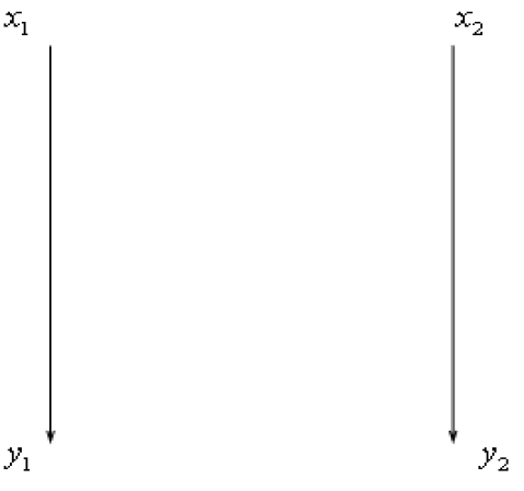
(a) $G_{1}$

(b) $G_{2}$

Figure 1. Unlike a traditional transport system $G_{1}$, a ramified transport system $G_{2}$ provides an exchange value.

As an illustration, we consider a spacial economy with two goods located at two distinct points $\left\{x_{1},x_{2}\right\}$ and two consumers living at two different locations $\left\{y_{1},y_{2}\right\}$. The spacial distribution is shown in Figure 1. Suppose consumer 1 favors good 2 more than good 1. However, good 2 may be more expensive than good 1 for some reason such as a higher transportation fee. As a result, she buys good 1 despite the fact that it is not her favorite. On the contrary, consumer 2 favors good 1 but ends up buying good 2, as good 1 is more expensive than good 2 for him. Given this purchase plan, a traditional transporter will ship the ordered items in a transport system like $G_{1}$ (see Figure 1a). However, as shown in [33] etc, a transport system like $G_{2}$ (see Figure 1b) with some branching structure might be more cost efficient than $G_{1}$. One may save some transportation cost by using a transport system like $G_{2}$ instead of $G_{1}$. Now, we observe another very interesting phenomenon about $G_{2}$. When using this transport system, one can simply switch the items which leads to consumer 1 getting good 2 and consumer 2 receives good 1. This exchange of items makes both consumers better off since they both get what they prefer. More importantly, no extra transportation cost is incurred during this exchange process. In other words, a ramified transport system like $G_{2}$ may possess an exchange value, which cannot be found in other transport systems like $G_{1}$.

The exchange value concept of a transport system that we propose here is valuable for both economics and mathematics. Existing market theories (e.g. [2], [12], [13], [14], [22], [23], [27], [30]) focus on the mechanism of exchanges between economic agents on an abstract market with relatively few discussions on its form. Our study complements the existing theories by showing that a transport system actually serves as a concrete market whose friction for exchange depends on the structure of the transport system as well as factors like preferences, prices, spatial distribution, etc. The existence of such an exchange value is due to the fact that the transport system provides a medium for potential exchange between agents. From the perspective of mathematical theory on optimal transport problem, our study provides another rationale for ramified structure which usually implies a potential exchange value. Furthermore, a new optimality criterion needs to be considered when building a transport system which leads to a new mathematical problem. Instead of simply minimizing the transportation cost, one might have to minimize the difference between transportation cost and exchange value.

The remainder of this paper is organized as follows. Section 2 describes the model environment with a brief review of consumer’s problem and related concepts from ramified optimal transportation. Sections 3 and 4 contain the main results of the paper. Section 3 proposes an explicit valuation formula to measure the exchange value for a given compatible transport system. The exchange value is defined by solving a maximization problem, which has a unique solution under suitable conditions. Criteria based on transport structures, preferences and prices are provided to determine the existence of a positive exchange value. We show that a reasonable combinations of these factors guarantees a positive exchange value. Section 4 studies a new optimal transport problem with an objective taking into account of both transportation cost and exchange value.

In this paper, we will use the following notations:

• $X$: a compact convex subset of a Euclidean space $\mathbb{R}^{m}$.

• $\mathbb{R}_{+}^{k}$: a subset of $\mathbb{R}^{k}$ defined as $\left\{\left(x_{1},...,x_{k}\right)\in\mathbb{R}^{k}:x_{i}\geq 0,\text{ }i=1,...,k\right\}.$

• $\mathbb{R}_{++}^{k}$: a subset of $\mathbb{R}^{k}$ defined as $\left\{\left(x_{1},...,x_{k}\right)\in\mathbb{R}^{k}:x_{i}>0,\text{ }i=1,...,k\right\}.$

• $p_{j}$: a price vector in $\mathbb{R}_{++}^{k}$ faced by consumer $j$ , $j=1,...,\ell.$

• $q_{j}$: a consumption vector in $\mathbb{R}_{+}^{k}$ of consumer $j$, $j=1,...,\ell.$

• $\mathcal{E}$: an economy as defined in (2.1).

• $\bar{q}$: the consumption plan as defined in (2.2).

• $e_{j}\left(p_{j},\tilde{u}_{j}\right)$: the expenditure function of consumer $j$, $j=1,...,\ell$, as defined in (2.3).

• $\mathbf{a}$: the atomic measure representing sources of goods, see ( 2.4).

• $\mathbf{b}$: the atomic measure representing consumers, see (2.5).

• $G$: a transport path from $\mathbf{a}$ to $\mathbf{b}$.

• $q$: a transport plan from $\mathbf{a}$ to $\mathbf{b}$.

• $S(q)$: the total expenditure function as defined in (3.1).

• $\Omega\left(\bar{q}\right)$: the set of all transport paths compatible with $\bar{q}$, as defined in (3.2).

• $\mathcal{F}_{G}$: the set of all feasible transport plans of $G$ as defined in (3.3).

• $\mathcal{V}\left(G\right)$: the exchange value of a transport path $G$, as defined in (3.7).

• $\mathbf{M}_{\alpha}\left(G\right)$: the transportation cost of a transport path $G$ as defined in (4.1).

2. Consumer’s Problem and Ramified Optimal Transportation

2.1. Consumer’s Problem

Suppose there are $k$ sources of different goods which could be purchased by $\ell$ consumers distributed on $X$. Each source $x_{i}\in X$ supplies only one type of goods, $i=1,...,k$. Each consumer $j$ located at $y_{j}\in X$ derives utility from consuming $k$ goods according to a utility function $u_{j}:\mathbb{R}_{+}^{k}\rightarrow\mathbb{R}:\left(q_{1j},...,q_{kj}\right)\mapsto u_{j},$ $j=1,...,\ell,$ where $u_{j}:\mathbb{R}_{+}^{k}\rightarrow\mathbb{R}$ is continuous, concave and increasing, $j=1,...,\ell.$ Each consumer $j$ has an initial wealth $w_{j}>0$ and faces a price vector $p_{j}=\left(p_{1j},...,p_{kj}\right)\in\mathbb{R}_{++}^{k},$ $j=1,...,k.$ We allow the prices to vary across consumers to accommodate the situation where consumers on different locations may have to pay different prices for the same good. This variation could be possibly due to different transportation fees. We denote this economy as

(2.1) $$\mathcal{E}=\left(U,P,W;x,y\right).$$

Now, we give a brief review of a consumer’s decision problem. Discussions of these materials can be found in most advanced microeconomics texts (e.g. [27]). Each consumer $j$ will choose an utility maximizing consumption plan given the price $p_{j}$ and wealth $w_{j}.$ More precisely, the consumption plan $\bar{q}_{j}$ is derived from the following utility maximizing problem:

(2.2) $$\bar{q}_{j}\in\arg\max\left\{u_{j}\left(q_{j}\right)\text{ }|\text{ }q_{j}\in\mathbb{R}_{+}^{k},\text{ }p_{j}\cdot q_{j}\leq w_{j}\right\}.$$

Given the continuity and concavity of $u_{j},$ we know this problem has a solution.

As will be used in defining the exchange value, we also consider the expenditure minimizing problem for a given utility level $\tilde{u}_{j}>u_{j}\left(\mathbf{0}\right)$:

(2.3) $$e_{j}\left(p_{j},\tilde{u}_{j}\right)=\min\left\{p_{j}\cdot q_{j}\text{ }|\text{ }q_{j}\in\mathbb{R}_{+}^{k},\text{ }u_{j}\left(q_{j}\right)\geq\tilde{u}_{j}\right\},$$

which is actually a problem dual to the above utility maximization problem. The continuity and concavity of $u_{j}$ guarantee a solution to this minimization problem. Here, $e_{j}\left(p_{j},\tilde{u}_{j}\right)$ represents the minimal expenditure needed for consumer $j$ to reach a utility level $\tilde{u}_{j}.$ Since $\tilde{u}_{j}>u_{j}\left(\mathbf{0}\right)$, we know that $e_{j}\left(p_{j},\tilde{u}_{j}\right)>0.$ Lemma 2.1 (see [27]) shows several standard properties of the expenditure function $e_{j}$.

Lemma 2.1.

Suppose that $u_{j}$ is a continuous, increasing utility function on $\mathbb{R}_{+}^{k}.$ The expenditure function $e_{j}\left(p_{j},\tilde{u}_{j}\right)$ is

1. Homogeneous of degree one in $p_{j}.$

2. Strictly increasing in $\tilde{u}_{j}$ and nondecreasing in $p_{ij}$ for any $i=1,...,k.$

3. Concave in $p_{j}.$

4. Continuous in $p_{j}$ and $\tilde{u}_{j}.$

The following lemma shows a nice property of $e_{j}$ when $u_{j}$ is homogeneous. This property will be used in the next section to characterize the solution set of the maximization problem defining exchange value.

Lemma 2.2.

If $u_{j}:\mathbb{R}_{+}^{k}\rightarrow\mathbb{R}$ is homogeneous of degree $\beta_{j}>0$, then $e_{j}\left(p_{j},\tilde{u}_{j}\right)$ is homogeneous of degree $\frac{1}{\beta_{j}}$ in $\tilde{u}_{j}$, which implies

$$e_{j}\left(p_{j},\tilde{u}_{j}\right)=e_{j}\left(p_{j},1\right)\left(\tilde{u}_{j}\right)^{\frac{1}{\beta_{j}}}.$$

Proof.

For any $\lambda>0$, since $u_{j}$ is homogeneous of degree $\beta_{j}$, we have

$$e_{j}\left(p_{j},\lambda\tilde{u}_{j}\right) = \min\left\{p_{j}\cdot q_{j}\text{ }|\text{ }q_{j}\in\mathbb{R}_{+}^{k},\text{ }u_{j}\left(q_{j}\right)\geq\lambda\tilde{u}_{j}\right\}$$

$$= \min\left\{p_{j}\cdot q_{j}\text{ }|\text{ }q_{j}\in\mathbb{R}_{+}^{k},\text{ }u_{j}\left(\left(1/\lambda\right)^{1/\beta_{j}}q_{j}\right)\geq\tilde{u}_{j}\right\}$$

$$= \min\left\{\left(\lambda\right)^{1/\beta_{j}}p_{j}\cdot\tilde{q}_{j}\text{ }|\text{ }\tilde{q}_{j}\in\mathbb{R}_{+}^{k}\text{, }u_{j}\left(\tilde{q}_{j}\right)\geq\tilde{u}_{j}\right\}\text{, where }\tilde{q}_{j}=(1/\lambda)^{1/\beta_{j}}q_{j},$$

$$= \left(\lambda\right)^{1/\beta_{j}}e_{j}\left(p_{j},\tilde{u}_{j}\right).$$

Therefore, $e_{j}\left(p_{j},\tilde{u}_{j}\right)$ is homogeneous of degree $\frac{1}{\beta_{j}}$ in $\tilde{u}_{j}.$ ∎

2.2. Ramified Optimal Transportation

Let $X$ be a compact convex subset of a Euclidean space $\mathbb{R}^{m}$. Recall that a Radon measure $\mathbf{a}$ on $X$ is atomic if $\mathbf{a}$ is a finite sum of Dirac measures with positive multiplicities. That is

$$\mathbf{a}=\sum\limits_{i=1}^{k}m_{i}\delta_{x_{i}}$$

for some integer $k\geq 1$ and some points $x_{i}\in X$, $m_{i}>0$ for each $i=1,\cdots,k$.

In the environment of the previous section, the $k$ sources of goods can be represented as an atomic measure on $X$ by

(2.4) $$\mathbf{a}=\sum\limits_{i=1}^{k}m_{i}\delta_{x_{i}},\text{ where }m_{i}=\sum_{j=1}^{\ell}\bar{q}_{ij}\text{,}$$

where $\bar{q}_{j}=\left(\bar{q}_{1j},\cdots,q_{kj}\right)$ is given by (2.2). Also, the $\ell$ consumers can be represented by another atomic measure on $X$ by

(2.5) $$\mathbf{b}=\sum\limits_{j=1}^{\ell}n_{j}\delta_{y_{j}}\text{, where }n_{j}=\sum_{i=1}^{k}\bar{q}_{ij}\text{.}$$

Without loss of generality, we may assume that

$$\sum_{ij}\bar{q}_{ij}=1,$$

and thus both $\mathbf{a}$ and $\mathbf{b}$ are probability measures on $X$.

Definition 2.1.

([33]) A transport path from $\mathbf{a}$ to $\mathbf{b}$ is a weighted directed graph $G$ consists of a vertex set $V\left(G\right)$, a directed edge set $E\left(G\right)$ and a weight function $w:E\left(G\right)\rightarrow\left(0,+\infty\right)$ such that $\{x_{1},x_{2},...,x_{k}\}\cup\{y_{1},y_{2},...,y_{\ell}\}\subseteq V(G)$ and for any vertex $v\in V(G)$, there is a balance equation

(2.6) $$\sum_{e\in E(G),e^{-}=v}w(e)=\sum_{e\in E(G),e^{+}=v}w(e)+\left\{\begin{array}[]{c}m_{i},\text{\ if }v=x_{i}\text{\ for some }i=1,...,k\\ -n_{j},\text{\ if }v=y_{j}\text{\ for some }j=1,...,\ell\\ 0,\text{\ otherwise }\end{array}\right.$$

where each edge $e\in E\left(G\right)$ is a line segment from the starting endpoint $e^{-}$ to the ending endpoint $e^{+}$.

Note that the balance equation (2.6) simply means the conservation of mass at each vertex. Viewing $G$ as a one dimensional polyhedral chain, we have the equation $\partial G=b-a$.

Let

$$Path\left(\mathbf{a,b}\right)$$

be the space of all transport paths from $\mathbf{a}$ to $\mathbf{b}$.

Definition 2.2.

(e.g. [1], [31]) A transport plan from $\mathbf{a}$ to $\mathbf{b}$ is an atomic probability measure

(2.7) $$q=\sum_{i=1}^{k}\sum_{j=1}^{\ell}q_{ij}\delta_{\left(x_{i},y_{j}\right)}$$

in the product space $X\times X$ such that

(2.8) $$\sum_{i=1}^{k}q_{ij}=n_{j}\text{ and }\sum_{j=1}^{\ell}q_{ij}=m_{i}$$

for each $i$ and $j$. Denote $Plan\left(\mathbf{a},\mathbf{b}\right)$ as the space of all transport plans from $\mathbf{a}$ to $\mathbf{b}$.

For instance, the $\bar{q}$ given by (2.2) is a transport plan in $Plan\left(\mathbf{a,b}\right)$.

Now, we want to consider the compatibility between a pair of transport path and transport plan ([33], [7]). Let $G$ be a given transport path in $Path\left(\mathbf{a,b}\right)$. From now on, we assume that for each $x_{i}$ and $y_{j}$, there exists at most one directed polyhedral curve $g_{ij}$ from $x_{i}$ to $y_{j}$. In other words, there exists a list of distinct vertices

(2.9) $$V\left(g_{ij}\right):=\left\{v_{i_{1}},v_{i_{2}},\cdots,v_{i_{h}}\right\}$$

in $V\left(G\right)$ with $x_{i}=v_{i_{1}}$, $y_{j}=v_{i_{h}}$, and each $\left[v_{i_{t}},v_{i_{t+1}}\right]$ is a directed edge in $E\left(G\right)$ for each $t=1,2,\cdots,h-1$. For some pairs of $\left(i,j\right)$, such a curve $g_{ij}$ from $x_{i}$ to $y_{j}$ may fail to exist, due to reasons like geographical barriers, law restrictions, etc. If such curve does not exists, we set $g_{ij}=0$ to denote the empty directed polyhedral curve. By doing so, we construct a matrix

(2.10) $$g=\left(g_{ij}\right)_{k\times\ell}$$

with each element of $g$ being a polyhedral curve. A very simple example satisfying these conditions is illustrated in Figure 2.

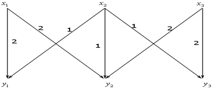
Figure 2. A transport path from $4\delta_{x_{1}}+3\delta_{x_{2}}+4\delta_{x_{3}}$ to $3\delta_{y_{1}}+5\delta_{y_{2}}+3\delta_{y_{3}}$ with $g_{13}=0,g_{31}=0$.

Definition 2.3.

A pair $\left(G,q\right)$ of a transport path $G\in Path\left(\mathbf{a,b}\right)$ and a transport plan $q\in Plan\left(\mathbf{a,b}\right)$ is compatible if $q_{ij}=0$ whenever $g_{ij}$ does not exist and

(2.11) $$G=q\cdot g.$$

Here, the equation (2.11) means

$$G=\sum_{i=1}^{k}\sum_{j=1}^{\ell}q_{ij}g_{ij}.$$

In terms of edges, it says that for each edge $e\in E\left(G\right)$, we have

$$\sum_{e\subseteq g_{ij}}q_{ij}=w\left(e\right).$$

Example 2.1.

Let $x^{\ast}\in X\setminus\left\{x_{1},\cdots,x_{k},y_{1},\cdots,y_{\ell}\right\}$. We may construct a path $\bar{G}\in Path\left(\mathbf{a,b}\right)$ as follows. Let

$$V\left(\bar{G}\right) = \left\{x_{1},\cdots,x_{k}\right\}\cup\left\{y_{1},\cdots,y_{\ell}\right\}\cup\left\{x^{\ast}\right\},$$

$$E\left(\bar{G}\right) = \left\{\left[x_{i},x^{\ast}\right]:i=1,\cdots,k\right\}\cup\left\{\left[x^{\ast},y_{j}\right]:j=1,\cdots,\ell\right\},$$

and

$$w\left(\left[x_{i},x^{\ast}\right]\right)=m_{i},w\left(\left[x^{\ast},y_{j}\right]\right)=n_{j}$$

for each $i$ and $j$. In this case, each $g_{ij}$ is the union of two edges $\left[x_{i},x^{\ast}\right]\cup\left[x^{\ast},y_{j}\right]$. Then, each transport plan $q\in Plan\left(\mathbf{a,b}\right)$ is compatible with $\bar{G}$ because

$$\sum_{\left[x_{i^{\ast}},x^{\ast}\right]\subseteq g_{ij}}q_{ij}=\sum_{j=1}^{\ell}q_{i^{\ast}j}=m_{i^{\ast}}=w\left(\left[x_{i^{\ast}},x^{\ast}\right]\right)$$

and

$$\sum_{\left[x^{\ast},y_{j^{\ast}}\right]\subseteq g_{ij}}q_{ij}=\sum_{i=1}^{k}q_{ij^{\ast}}=n_{j^{\ast}}=w\left(\left[x^{\ast},y_{j^{\ast}}\right]\right).$$

3. Exchange Value Of A Transport system

In a transport system, a transporter can simply ship the desired bundle to consumers as they have initially planned. This is a universal strategy. However, we will see that allowing the exchange of goods between consumers may make them better off without incurring any additional transportation cost. In other words, there is an exchange value embedded in some transport system.

3.1. Exchange Value

For each probability measure $q=\left(q_{ij}\right)\in\mathcal{P}\left(X\times X\right)$, we define

(3.1) $$S\left(q\right)=\sum_{j=1}^{\ell}e_{j}\left(p_{j},u_{j}\left(q_{j}\right)\right)=\sum_{j=1}^{\ell}\min\left\{p_{j}\cdot t_{j}\text{ }|\text{ }t_{j}\in\mathbb{R}_{+}^{k},\text{ }u_{j}\left(t_{j}\right)\geq u_{j}\left(q_{j}\right)\right\},$$

where $q_{j}=\left(q_{1j},q_{2j},...,q_{kj}\right)$ for each $j=1,\cdots,\ell$. Here, $S\left(q\right)$ represents the least total expenditure for each individual $j$ to reach utility level $u_{j}\left(q_{j}\right).$ One can simply use Lemmas 2.1 and 2.2 to prove the following lemma which shows several properties of this function $S.$

Lemma 3.1.

Suppose each $u_{j}$ is continuous, concave, and increasing on $\mathbb{R}_{+}^{k},$ $j=1,...,\ell.$ The function $S\left(q\right)$ is

1. Homogeneous of degree one in $p=\left(p_{1},...,p_{\ell}\right).$

2. Increasing in $q$ and nondecreasing in $p_{ij}$ for any $i=1,...,k,$ $j=1,...,\ell.$

3. Concave in $p.$

4. Continuous in $p$ and $q.$

Let $\bar{q}\in Plan\left(\mathbf{a,b}\right)$ be the initial plan given by (2.2). Denote

(3.2) $$\Omega\left(\bar{q}\right)=\left\{G\in Path\left(\mathbf{a,b}\right)\text{ }|\text{ }\left(G,\bar{q}\right)\text{ is compatible}\right\}.$$

Let $G\in\Omega\left(\bar{q}\right)$ be fixed and $g=\left(g_{ij}\right)$ be the corresponding matrix of $G$ as given in (2.10). That is,

$$G=g\cdot\bar{q}.$$

Then, we introduce the following definition:

Definition 3.1.

Each transport plan in the set

(3.3) $$\mathcal{F}_{G}=\left\{q\in\mathcal{P}\left(X\times X\right)\left|\begin{array}[]{c}q\text{ is compatible with }G\\ u_{j}\left(q_{j}\right)\geq u_{j}\left(\bar{q}_{j}\right),\text{ }j=1,...,\ell.\end{array}\right.\right\}$$

is called a feasible plan for $G.$

Recall that $q$ is compatible with $G$ means that

(3.4) $$q_{ij}=0\text{ if }g_{ij}\text{ does not exist}$$

and

$$g\cdot q=g\cdot\bar{q},$$

in the sense that for each edge $e\in E\left(G\right)$, we have an equality

(3.5) $$\sum_{e\subseteq g_{ij}}q_{ij}=w\left(e\right)\text{, where }w\left(e\right)=\sum_{e\subseteq g_{ij}}\bar{q}_{ij}.$$

For any feasible plan $q\in\mathcal{F}_{G}$, the constraint $u_{j}\left(q_{j}\right)\geq u_{j}\left(\bar{q}_{j}\right)$ means that $q_{j}$ is at least as good as $\bar{q}_{j}$ for each consumer $j$.

Since $\bar{q}\in Plan\left(\mathbf{a,b}\right)$, the compatibility condition automatically implies that $q\in Plan\left(\mathbf{a,b}\right)$ whenever $q\in\mathcal{F}_{G}$.

Lemma 3.2.

$\mathcal{F}_{G}$ is a nonempty, convex and compact subset of $\mathcal{P}\left(X\times X\right).$

Proof.

Clearly, $\bar{q}\in\mathcal{F}_{G},$ showing that $\mathcal{F}_{G}\neq\emptyset.$ The set $\mathcal{F}_{G}$ is convex since it is an intersection of two convex sets $\left\{q\in\mathcal{P}\left(X\times X\right)\text{ }|\text{ }g\cdot q=G\text{ }\right\}$ and $\prod\nolimits_{j=1}^{\ell}\left\{q_{j}\in\mathcal{P}\left(X\times X\right)\left|u_{j}\left(q_{j}\right)\geq u_{j}\left(\bar{q}_{j}\right)\right.\right\},$ where the convexity of $\left\{q_{j}\in\mathcal{P}\left(X\times X\right)\left|u_{j}\left(q_{j}\right)\geq u_{j}\left(\bar{q}_{j}\right)\right.\right\}$ comes from the concavity of $u_{j}$, $j=1,...,\ell.$ Since each $u_{j}$ is continuous, we have $\mathcal{F}_{G}$ is a closed subset of $\mathcal{P}\left(X\times X\right)$ and hence it is compact. ∎

Note that when $G=\bar{G}$ as constructed in the example 2.1, we have

$$\mathcal{F}_{\bar{G}}=\left\{q\in Plan\left(\mathbf{a,b}\right)\left|u_{j}\left(q_{j}\right)\geq u_{j}\left(\bar{q}_{j}\right),\text{ }j=1,...,\ell\right.\right\}.$$

Clearly, for each $G\in Path\left(\mathbf{a,b}\right)$, we have

(3.6) $$\bar{q}\in\mathcal{F}_{G}\subseteq\mathcal{F}_{\bar{G}}.$$

Definition 3.2.

Let $\mathcal{E}$ be an economy as in (2.1). For each transport path $G\in\Omega\left(\bar{q}\right)$, we define the exchange value of $G$ by

(3.7) $$\mathcal{V}\left(G;\mathcal{E}\right)=\underset{q\in\mathcal{F}_{G}}{\max}\text{ }S\left(q\right)-S\left(\bar{q}\right),$$

where $S$ is given by (3.1). Without causing confusion, we may simply denote $\mathcal{V}\left(G;\mathcal{E}\right)$ by $\mathcal{V}\left(G\right)$.

Since $S$ is a continuous function on a compact set, the exchange value function $\mathcal{V}:\Omega\rightarrow[0,\infty)$ is well defined. Furthermore, for each $q\in\mathcal{F}_{G}$, given $u_{j}\left(q_{j}\right)\geq u_{j}\left(\bar{q}_{j}\right)$ for all $j$, we have

(3.8) $$S\left(q\right)\geq S\left(\bar{q}\right).$$

Remark 1.

Our way of defining the feasibility set $\mathcal{F}_{G}$ guarantees that the exchange value is not obtained at the cost of increasing transportation cost. This is because the compatibility condition ensures that replacing $\bar{q}$ by any feasible plan $q\in\mathcal{F}_{G}$ will not change the transportation cost $M_{\alpha}\left(G\right)$ (to be defined later in (4.1)), as the quantity on each edge $e$ of $G$ is set to be $w\left(e\right)$.

The following proposition shows that the exchange value is always nonnegative and bounded from above.

Proposition 3.1.

For any $G\in\Omega\left(\bar{q}\right),$

$$0\leq\mathcal{V}\left(G\right)\leq\mathcal{V}\left(\bar{G}\right).$$

Proof.

This follows from the definition as well as (3.6). ∎

Example 3.1.

Let’s return to the example discussed in introduction. More precisely, suppose $u_{1}\left(q_{11},q_{21}\right)=q_{11}+3q_{21},$ $w_{1}=1/2,$ $p_{1}=\left(1,6\right)$ and $u_{2}\left(q_{12},q_{22}\right)=3q_{12}+q_{22},$ $w_{2}=1/2,$ $p_{2}=\left(6,1\right).$ By solving (2.2), i.e.

$$\bar{q}_{1} \in \arg\max\left\{u_{1}\left(q_{11},q_{21}\right)\text{ }|\text{ }p_{1}\cdot q_{1}\leq w_{1}\right\}$$

$$= \arg\max\left\{q_{11}+3q_{21}\text{ }|\text{ }q_{11}+6q_{21}\leq 1/2\right\}$$

$$= \left\{\left(1/2,0\right)\right\},$$

we find  $\bar{q}_{1}=\left(1/2,0\right)$. Similarly, we have $\bar{q}_{2}=\left(0,1/2\right)$. This gives the initial plan

$$\bar{q}=\left(\begin{array}[]{cc}1/2&0\\ 0&1/2\end{array}\right).$$

Now, solving expenditure minimization problems (2.3) yields

$$e_{1}\left(p_{1},\tilde{u}_{1}\right) = \min\left\{p_{1}\cdot q_{1}\text{ }|\text{ }q_{1}\in\mathbb{R}_{+}^{2},u_{1}\left(q_{1}\right)\geq\tilde{u}_{1}\right\}$$

$$= \min\left\{q_{11}+6q_{21}\text{ }|\text{ }\left(q_{11},q_{21}\right)\in\mathbb{R}_{+}^{2},q_{11}+3q_{21}\geq\tilde{u}_{1}\right\}$$

$$= \tilde{u}_{1}.$$

Similarly, we have $e_{2}\left(p_{2},\tilde{u_{2}}\right)=\tilde{u_{2}}$. From these, we get

$$S\left(q\right)=e_{1}\left(p_{1},u_{1}\left(q_{1}\right)\right)+e_{2}\left(p_{2},u_{2}\left(q_{2}\right)\right)=u_{1}\left(q_{1}\right)+u_{2}\left(q_{2}\right)$$

for each probability measure $q\in\mathcal{P}\left(X\times X\right)$. Now, we find the exchange value embedded in the transport systems $G_{1}$ and $G_{2}$ as given in Figure 1.

• $G_{1}:$ The associated feasible set is

  $$\mathcal{F}_{G_{1}}=\left\{q=\left(\begin{array}[]{cc}q_{11}&q_{12}\\ q_{21}&q_{22}\end{array}\right)\in\mathcal{P}\left(X\times X\right)\left|\begin{array}[]{c}q_{11}=1/2,\text{ }q_{21}=0,\text{ }q_{12}=0,\text{ }q_{22}=1/2,\\ q_{11}+3q_{21}\geq u_{1}\left(\bar{q}_{1}\right)=1/2,\\ \text{ }3q_{12}+q_{22}\geq u_{2}\left(\bar{q}_{2}\right)=1/2.\end{array}\right.\right\}=\left\{\bar{q}\right\}.$$

  Thus, the exchange value of $G_{1}$ is

  $$\mathcal{V}\left(G_{1}\right)=\underset{q\in\mathcal{F}_{G_{1}}}{\max}S\left(q\right)-S\left(\bar{q}\right)=S\left(\bar{q}\right)-S\left(\bar{q}\right)=0.$$

• $G_{2}:$ The associated feasible set is

  $$\mathcal{F}_{G_{2}} = \left\{q=\left(\begin{array}[]{cc}q_{11}&q_{12}\\ q_{21}&q_{22}\end{array}\right)\in\mathcal{P}\left(X\times X\right)\left|\begin{array}[]{c}q_{11}+q_{12}=1/2,q_{21}+q_{22}=1/2,\\ q_{11}+q_{21}=1/2,\\ q_{11}+3q_{21}\geq u_{1}\left(\bar{q}_{1}\right)=1/2,\\ \text{ }3q_{12}+q_{22}\geq u_{2}\left(\bar{q}_{2}\right)=1/2.\end{array}\right.\right\}$$

  $$= \left\{q=\left(\begin{array}[]{cc}q_{11}&1/2-q_{11}\\ 1/2-q_{11}&q_{11}\end{array}\right)\left|\begin{array}[]{c}q_{11}\leq 1/2\\ \text{ }q_{11}\geq 0\end{array}\right..\right\}$$

  Thus, we have the following exchange value

  $$\mathcal{V}\left(G_{2}\right) = \underset{q\in\mathcal{F}_{G_{2}}}{\max}S\left(q\right)-S\left(\bar{q}\right)$$

  $$= \underset{q\in\mathcal{F}_{G_{2}}}{\max}\left\{\left(q_{11}+3q_{21}\right)+\left(3q_{12}+q_{22}\right)\right\}-1$$

  $$= \underset{0\leq q_{11}\leq\frac{1}{2}}{\max}\left\{\left(q_{11}+3\left(1/2-q_{11}\right)\right)+\left(3\left(1/2-q_{11}\right)+q_{11}\right)\right\}-1$$

  $$= \underset{0\leq q_{11}\leq\frac{1}{2}}{\max}\left\{3-4q_{11}\right\}-1=2.$$

Basically, there are three factors affecting the size of exchange value: transport structures, preferences and prices. In the rest of this section, we will study how these three factors affect the exchange value.

3.2. Transport Structures and Exchange Value

For any $G\in\Omega\left(\bar{q}\right)$, define

$$K\left(\bar{q},G\right)=\left\{q\in\mathcal{P}\left(X\times X\right)\left|q\text{ is compatible with }G\right.\right\},$$

and

$$U\left(\bar{q}\right)=\left\{q\in\mathcal{P}\left(X\times X\right)\left|u_{j}\left(q_{j}\right)\geq u_{j}\left(\bar{q}_{j}\right),\text{ }j=1,...,\ell.\right.\right\}$$

Then,

$$\mathcal{F}_{G}=K\left(\bar{q},G\right)\cap U\left(\bar{q}\right).$$

Clearly, the structure of a transport system influences the exchange value through $K\left(\bar{q},G\right).$ For this consideration, this subsection will focus on the properties of $K\left(\bar{q},G\right)$ whose implications on exchange value will be self-evident in the following subsections.

Proposition 3.2.

$K\left(\bar{q},G\right)$ is a polygon of dimension $N\left(G\right)+\chi\left(G\right)-\left(k+\ell\right)$, where $\chi\left(G\right)$ is the Euler Characteristic number of $G$, and $N\left(G\right)$ is the total number of existing $g_{ij}$’s in $G$.

Proof.

For each interior vertex $v$ of $G$, let $\left\{e_{1},e_{2},\cdots,e_{h}\right\}\subseteq E\left(G\right)$ be the set of edges with $e_{i}^{-}=v$. Then, each $e_{i}$ corresponds to an equation of the form (3.5). Nevertheless, due to the balance equation (2.6), we may remove one redundant equation from these $h$ equations. As a result, the total number of equations of the form (3.5) equals the total number of edges of $G$ minus the total number of interior vertices of $G$. Thus, $K\left(\bar{q},G\right)$ is defined by $k+\ell-\chi\left(G\right)$ number of linear equations in the form of (3.5), and $\left(k\ell-N\left(G\right)\right)$ number of equations (3.4). This shows that $K\left(\bar{q},G\right)$ is a convex polygon of dimension

(3.11) $$\dim\left(K\left(\bar{q},G\right)\right)\geq k\ell-\left(k+\ell-\chi\left(G\right)\right)-\left(k\ell-N\left(G\right)\right)=N\left(G\right)+\chi\left(G\right)-\left(k+\ell\right).$$

By the following Lemma 3.3, we have an inequality of the other direction. ∎

Lemma 3.3.

The dimension of $K\left(\bar{q},G\right)$ is no more than $N\left(G\right)+\chi\left(G\right)-\left(k+\ell\right)$.

Proof.

Since $K\left(\bar{q},G\right)$ is defined by $k\ell$ variables $\left(q_{ij}\right)_{k\times\ell}$ which satisfy equations (3.4) and (3.5). As the number of equations (3.4) is $k\ell-N\left(G\right)$, it is sufficient to show that

$$rank\left(A\right)\geq k\ell-\left(k\ell-N\left(G\right)\right)-\left(N\left(G\right)+\chi\left(G\right)-\left(k+\ell\right)\right)=\left(k+\ell-\chi\left(G\right)\right),$$

where $A$ is the coefficient matrix given by linear equations (3.5). We prove this by using induction on the number $k$. When $k=1$, then the coefficient matrix $A^{\left(1\right)}$ is in the form of

$$A^{\left(1\right)}=\left(\begin{array}[]{c}I\\ B\end{array}\right),$$

where $I$ is the $N\left(G^{\left(1\right)}\right)\times N\left(G^{\left(1\right)}\right)$ identity matrix $I_{N\left(G^{\left(1\right)}\right)}$, and $B$ is some matrix of $N\left(G^{\left(1\right)}\right)$ columns. Thus, the rank of $A^{\left(1\right)}$ is $N\left(G^{\left(1\right)}\right)$. On the other hand, the Euler Characteristic number of $G^{\left(1\right)}$ is

$$\chi\left(G^{\left(1\right)}\right)=1+\left(\ell-N\left(G^{\left(1\right)}\right)\right)\text{,}$$

which gives

(3.12) $$rank\left(A^{\left(1\right)}\right)=\left(1+\ell\right)-\chi\left(G^{\left(1\right)}\right).$$

Now, we may use induction by assuming that

(3.13) $$rank\left(A^{\left(k\right)}\right)\geq\left(k+\ell\right)-\chi\left(G^{\left(k\right)}\right)$$

for any $G^{\left(k\right)}$ from $k$ sources to $\ell$ consumers. We want to show that

$$rank\left(A^{\left(k+1\right)}\right)\geq\left(k+\ell+1\right)-\chi\left(G^{\left(k+1\right)}\right)$$

for any $G^{\left(k+1\right)}$ from $\left(k+1\right)$ sources to $\ell$ consumers.

Let

$$E_{1}^{\left(k+1\right)} = \left\{e\in E\left(G^{\left(k+1\right)}\right):e\subseteq g_{ij}\text{ for some }i\in\left\{1,\cdots,k\right\}\text{ and }j\in\left\{1,\cdots,\ell\right\}\right\}$$

$$E_{2}^{\left(k+1\right)} = E\left(G^{\left(k+1\right)}\right)\setminus E_{1}^{\left(k+1\right)}.$$

For each $e\in E_{2}^{\left(k+1\right)}$, we know $e\subseteq g_{\left(k+1\right)j}$ for some $j\in\left\{1,\cdots,\ell\right\}$, but $e\notin E_{1}^{\left(k+1\right)}$. Then, for each $e\in E_{1}^{\left(k+1\right)}$, we have

$$\sum_{\begin{subarray}{c}1\leq i\leq k,1\leq j\leq\ell\\ e\subseteq g_{ij}\end{subarray}}q_{ij}+\sum_{\begin{subarray}{c}1\leq j\leq\ell\\ e\subseteq g_{\left(k+1\right)j}\end{subarray}}q_{\left(k+1\right)j}=w\left(e\right).$$

Also, for each $e\in E_{2}^{\left(k+1\right)}$, we have

$$\sum_{\begin{subarray}{c}1\leq j\leq\ell\\ e\subseteq g_{\left(k+1\right)j}\end{subarray}}q_{\left(k+1\right)j}=w\left(e\right).$$

As a result, the matrix $A^{\left(k+1\right)}$ can be expressed in the form

(3.14) $$A^{\left(k+1\right)}=\left(\begin{array}[]{cc}A^{\left(k\right)}&B^{\left(k+1\right)}\\ 0&C^{\left(k+1\right)}\end{array}\right).$$

Now, we consider a new transport path

$$\tilde{G}=\sum_{e\in E_{2}^{\left(k+1\right)}}w\left(e\right)\left[e\right]\text{.}$$

from a single source (i.e. $x_{k+1}$) to a few (say $\tilde{\ell}$ ) targets (, which do not necessarily belong to the original consumers). The matrix $C^{\left(k+1\right)}$ here is the associated $A^{\left(1\right)}$ matrix for $\tilde{G}$, and thus has rank $\left(1+\tilde{\ell}\right)-\chi\left(\tilde{G}\right)=\tilde{\ell}$ as $\tilde{G}$ is contractible. Also, we have

$$\chi\left(G^{\left(k+1\right)}\right)=\chi\left(G^{\left(k\right)}\right)+1-\tilde{\ell}.$$

Therefore, by (3.13) and (3.14),

$$rank\left(A^{\left(k+1\right)}\right) \geq rank\left(A^{\left(k\right)}\right)+rank\left(C^{\left(k+1\right)}\right)$$

$$\geq \left(k+\ell\right)-\chi\left(G^{\left(k\right)}\right)+\left(1+\chi\left(G^{\left(k\right)}\right)-\chi\left(G^{\left(k+1\right)}\right)\right)$$

$$= \left(k+1+\ell\right)-\chi\left(G^{\left(k+1\right)}\right).$$

∎

Corollary 3.1.

Suppose $G\in\Omega\left(\bar{q}\right)$.

1. If $k+\ell\geq N\left(G\right)+\chi\left(G\right)$, then $\mathcal{F}_{G}=\left\{\bar{q}\right\}$.

2. If $k+\ell<N\left(G\right)+\chi\left(G\right)$ and $\bar{q}$ is an interior point of the polygon $K\left(\bar{q},G\right)$, then $\mathcal{F}_{G}$ is a convex set of positive dimension. In particular, $\mathcal{F}_{G}\neq\left\{\bar{q}\right\}.$

Proof.

If $k+\ell\geq N\left(G\right)+\chi\left(G\right)$, the convex polygon $K\left(\bar{q},G\right)$ becomes a dimension zero set, and thus $\mathcal{F}_{G}=\left\{\bar{q}\right\}$. When $k+\ell<N\left(G\right)+\chi\left(G\right)$, the polygon $K\left(\bar{q},G\right)$ has positive dimension. Since each $u_{j}$ is concave, $U\left(\bar{q}\right)$ is a convex set containing $\bar{q}$. When $\bar{q}$ is an interior point of $K\left(\bar{q},G\right)$, the intersection $\mathcal{F}_{G}=K\left(\bar{q},G\right)\cap U\left(\bar{q}\right)$ is still a convex set of positive dimension. Thus, $\mathcal{F}_{G}\neq\left\{\bar{q}\right\}$. ∎

Proposition 3.3.

Suppose $G\in\Omega\left(\bar{q}\right)$ satisfies the following condition: for any two pairs $\left(i_{1},i_{2}\right)$ with $i_{1}\neq i_{2}$ and $\left(j_{1},j_{2}\right)$ with $j_{1}\neq j_{2}$, we have

(3.15) $$V\left(g_{i_{1}j_{2}}\right)\cap V\left(g_{i_{2}j_{1}}\right)=\emptyset\text{,}$$

where $V\left(g_{ij}\right)$ is given in (2.9). Then, $k+\ell\geq N\left(G\right)+\chi\left(G\right)$. Hence, by Corollary 3.1, $\mathcal{F}_{G}$ is a singleton $\left\{\bar{q}\right\}$.

Proof.

We still use the notations that have been used in the proof of Lemma 3.3. When $k=1$, $\chi\left(G\right)=1+\ell-N\left(G\right)$, and thus $k+\ell=N\left(G\right)+\chi\left(G\right)$. By using induction, we assume that the result is true for any $k$ sources. We want to show that it holds for $k+1$ sources. Suppose there are totally $d$ edges of $G^{\left(k+1\right)}$ connecting the vertex $x_{k+1}$, then as discussed earlier, we may construct a transport path $\tilde{G}$  from a single source $x_{k+1}$ to a few targets $\left\{v_{1},v_{2},\cdots,v_{\tilde{\ell}}\right\}$ with $v_{i}\in V\left(G^{\left(k\right)}\right)$. For each $v_{j}$, it corresponds to a unique $g_{\left(k+1\right)j^{\ast}}$ for some $j^{\ast}\in\left\{1,2,\cdots,\ell\right\}$ that passing through the vertex $v_{j}$. Indeed, suppose both $g_{\left(k+1\right)j_{1}}$ and $g_{\left(k+1\right)j_{2}}$ passing through $v_{j}$ with $j_{1}\neq j_{2}$. Since $v_{j}\in V\left(G^{\left(k\right)}\right)$, there exists an $i^{\ast}\in\left\{1,2,\cdots,k\right\}$ such that $x_{i^{\ast}}$ and $v_{j}$ are connected by a directed curve lying in $G^{\left(k\right)}$. Then, $v_{j}\in g_{i^{\ast}j_{2}}\cap g_{\left(k+1\right)j_{1}}$, which contradicts condition (3.15). As a result,

$$N\left(G^{\left(k+1\right)}\right)=N\left(G^{\left(k\right)}\right)+\tilde{\ell}.$$

On the other hand, it is easy to see that $\chi\left(G^{\left(k+1\right)}\right)=\chi\left(G^{\left(k\right)}\right)+1-\tilde{\ell}$. So, by induction,

$$\left(k+1\right)+\ell \geq 1+N\left(G^{\left(k\right)}\right)+\chi\left(G^{\left(k\right)}\right)$$

$$= 1+\left(N\left(G^{\left(k+1\right)}\right)-\tilde{\ell}\right)+\left(\chi\left(G^{\left(k+1\right)}\right)+\tilde{\ell}-1\right)=N\left(G^{\left(k+1\right)}\right)+\chi\left(G^{\left(k+1\right)}\right).$$

This shows that

$$k+\ell\geq N\left(G\right)+\chi\left(G\right)$$

for any $G$ satisfying condition (3.15). Therefore, $\mathcal{F}_{G}$ is a singleton $\left\{\bar{q}\right\}$. ∎

In Proposition 3.2, we will consider an inverse problem of Proposition 3.3 under some suitable conditions on the prices.

Given two transport paths

$$G_{1} = \left\{V\left(G_{1}\right),E\left(G_{1}\right),w_{1}:E\left(G_{1}\right)\rightarrow[0,+\infty)\right\}\text{ and}$$

$$G_{2} = \left\{V\left(G_{2}\right),E\left(G_{2}\right),w_{2}:E\left(G_{2}\right)\rightarrow[0,+\infty)\right\},$$

we say $G_{1}$ is topologically equivalent to $G_{2}$ if there exists a homeomorphism $h:X\rightarrow X$ such that

$$V\left(G_{2}\right) = h\left(V\left(G_{1}\right)\right),$$

$$E\left(G_{2}\right) = \left\{h\left(e\right):e\in E\left(G_{1}\right)\right\}$$

$$\text{ and }w_{2}\left(h\left(e\right)\right) = w_{1}\left(e\right)\text{ for each }e\in E\left(G_{1}\right)\text{.}$$

Clearly, if $G_{1}$ is topologically equivalent to $G_{2},$ then $K\left(\bar{q},G_{1}\right)=K\left(\bar{q},G_{2}\right)$. As a result, we know $\mathcal{V}$ is topologically invariant:

Proposition 3.4.

If $G_{1}$ is topologically equivalent to $G_{2}$, then $\mathcal{V}\left(G_{1}\right)=\mathcal{V}\left(G_{2}\right)$.

As will be clear in the next section, the topological invariance of $\mathcal{V}$ is a very useful result because it enables us to inherit many existing theories in ramified optimal transportation when studying a new optimal transport problem there.

3.3. Preferences and Exchange Value

In this subsection, we will study the implications of preferences, which are represented by utility functions, on the exchange value. The following proposition shows that there is no exchange value when all consumers derive their utilities solely from the total amount of goods they consume.

Proposition 3.5.

If $u_{j}:\mathbb{R}_{+}^{k}\rightarrow\mathbb{R}$ is of the form $u_{j}\left(q_{j}\right)=f_{j}\left(\sum_{i=1}^{k}q_{ij}\right)$ for some $f_{j}:[0,\infty)\rightarrow\mathbb{R}$ for each $j=1,...,\ell,$ then $\mathcal{V}\left(G\right)=0$ for any $G\in\Omega\left(\bar{q}\right)$.

Proof.

For any $q\in\mathcal{F}_{G},$ by compatibility, we know

$$\sum_{i=1}^{k}q_{ij}=\sum_{i=1}^{k}\bar{q}_{ij},\text{ }j=1,...,\ell,$$

which implies

$$u_{j}\left(q_{j}\right)=f_{j}\left(\sum_{i=1}^{k}q_{ij}\right)=f_{j}\left(\sum_{i=1}^{k}\bar{q}_{ij}\right)=u_{j}\left(\bar{q}_{j}\right),$$

showing that all consumers find any feasible plan indifferent to $\bar{q}.$ Therefore, we get

$$\mathcal{V}\left(G\right)=\underset{q\in\mathcal{F}_{G}}{\max}\text{ }S\left(q\right)-S\left(\bar{q}\right)=0.$$

∎

For any $G\in\Omega\left(\bar{q}\right)$, denote $Q\left(G\right)$ as the solution set of the maximization problem (3.7) defining exchange value, i.e.,

(3.16) $$Q\left(G\right)=\left\{\hat{q}\in\mathcal{F}_{G}\text{ }|\text{ }\mathcal{V}\left(G\right)=S\left(\hat{q}\right)-S\left(\bar{q}\right)\right\}.$$

We are interested in describing geometric properties of the set $Q\left(G\right)$. In particular, if $Q\left(G\right)$ contains only one element, then the problem (3.7) has a unique solution.

Proposition 3.6.

For any $G\in\Omega\left(\bar{q}\right),$

1. The solution set $Q\left(G\right)$ is a compact nonempty set.

2. If $u_{j}:\mathbb{R}_{+}^{k}\rightarrow\mathbb{R}$ is homogeneous of degree $\beta_{j}>0$ and $\left(u_{j}\left(q_{j}\right)\right)^{\frac{1}{\beta_{j}}}$ is concave in $q_{j},$ $j=1,...,\ell,$ then $Q\left(G\right)$ is convex.

3. (Uniqueness) If $u_{j}:\mathbb{R}_{+}^{k}\rightarrow\mathbb{R}$ is homogeneous of degree $\beta_{j}>0$ and$\ \left(u_{j}\left(q_{j}\right)\right)^{\frac{1}{\beta_{j}}}$ is concave in $q_{j}$ satisfying the condition

   (3.17) $$\left(u_{j}\left(\left(1-\lambda_{j}\right)\tilde{q}_{j}+\lambda_{j}\hat{q}_{j}\right)\right)^{\frac{1}{\beta_{j}}}>\left(1-\lambda_{j}\right)\left(u_{j}\left(\tilde{q}_{j}\right)\right)^{\frac{1}{\beta_{j}}}+\lambda_{j}\left(u_{j}\left(\hat{q}_{j}\right)\right)^{\frac{1}{\beta_{j}}}$$

   for each $\lambda_{j}\in\left(0,1\right)$, and any non-collinear $\tilde{q}_{j},\hat{q}_{j}\in\mathbb{R}_{+}^{k}$ , for each $j=1,...,\ell.$ Then $Q\left(G\right)$ is a singleton, and thus the problem (3.7) has a unique solution.

Proof.

Since the function $S\left(q\right)$ is continuous in $q$, $Q\left(G\right)$ becomes a closed subset of the compact set $\mathcal{F}_{G}$, and thus $Q\left(G\right)$ is also compact.

If $u_{j}:\mathbb{R}_{+}^{k}\rightarrow\mathbb{R}$ is homogeneous of degree $\beta_{j}>0$, then Lemma 2.2 implies that

(3.18) $$e_{j}\left(p_{j},u_{j}\left(q_{j}\right)\right)=e_{j}\left(p_{j},1\right)\left(u_{j}\left(q_{j}\right)\right)^{\frac{1}{\beta_{j}}}\text{ and }S\left(q\right)=\sum\nolimits_{j=1}^{\ell}e_{j}\left(p_{j},1\right)\left(u_{j}\left(q_{j}\right)\right)^{\frac{1}{\beta_{j}}}.$$

Thus, when each $\left(u_{j}\left(q_{j}\right)\right)^{\frac{1}{\beta_{j}}}$ is concave in $q_{j}$, we have $S$ is concave in $q$. Now, for any $q^{\ast},\tilde{q}\in Q\left(G\right)$ and $\lambda\in\left[0,1\right],$ the convexity of $\mathcal{F}_{G}$ implies $\left(1-\lambda\right)q^{\ast}+\lambda\tilde{q}\in$ $\mathcal{F}_{G}$ and the concavity of $S$ implies

(3.19) $$S\left(\left(1-\lambda\right)q^{\ast}+\lambda\tilde{q}\right)-S\left(\bar{q}\right)\geq\left(1-\lambda\right)\left(S\left(q^{\ast}\right)-S\left(\bar{q}\right)\right)+\lambda\left(S\left(\tilde{q}\right)-S\left(\bar{q}\right)\right)=\mathcal{V}\left(G\right),$$

showing that $\left(1-\lambda\right)q^{\ast}+\lambda\tilde{q}\in Q\left(G\right).$ Therefore, $Q\left(G\right)$ is convex.

To prove the uniqueness, we note that $\left(1-\lambda\right)q^{\ast}+\lambda\tilde{q}\in Q\left(G\right)$ implies an equality in (3.19), i.e.,

(3.20) $$\left(u_{j}\left(\left(1-\lambda\right)q_{j}^{\ast}+\lambda\tilde{q}_{j}\right)\right)^{\frac{1}{\beta_{j}}}=\left(1-\lambda\right)\left(u_{j}\left(q_{j}^{\ast}\right)\right)^{\frac{1}{\beta_{j}}}+\lambda\left(u_{j}\left(\tilde{q}_{j}\right)\right)^{\frac{1}{\beta_{j}}}$$

for each $\lambda\in\left(0,1\right)$, and each $j=1,2,\cdots,\ell$. When $\left(u_{j}\left(q_{j}\right)\right)^{\frac{1}{\beta_{j}}}$ is concave in $q_{j}$ and satisfies (3.17), the equality (3.20) implies that $q_{j}^{\ast}$ and $\tilde{q}_{j}$ are collinear in the sense that $q_{j}^{\ast}=t_{j}\tilde{q}_{j}$ for some $t_{j}\geq 0$. By (2.8),

$$n_{j}=\sum_{i}q_{ij}^{\ast}=\sum_{i}t_{j}\tilde{q}_{ij}=t_{j}\sum_{j}\tilde{q}_{ij}=t_{j}n_{j}.$$

Therefore, $t_{j}=1$ as $n_{j}>0$. This shows $q^{\ast}=\tilde{q}$ and thus $Q\left(G\right)$ is a singleton with an element $\tilde{q}.$ ∎

Two classes of utility functions widely used in economics satisfy conditions in Proposition (3.6). One is Cobb-Douglas function ([27])

$$u:\mathbb{R}_{+}^{k}\rightarrow\mathbb{R}:u\left(q_{1},...,q_{k}\right)=\prod\limits_{i=1}^{k}\left(q_{i}\right)^{\tau_{i}},\text{ }\tau_{i}>0,\text{ }i=1,...,k.$$

The other is Constant Elasticity of Substitution function ([27])

$$u:\mathbb{R}_{+}^{k}\rightarrow\mathbb{R}:u\left(q_{1},...,q_{k}\right)=\left[\sum_{i=1}^{k}\gamma_{i}\left(q_{i}\right)^{\tau}\right]^{\frac{\beta}{\tau}},\text{ }\tau\in(0,1),\text{ }\beta>0,\text{ }\gamma_{i}>0,\text{ }i=1,...,k.$$

Proposition 3.7.

Suppose $u_{j}:\mathbb{R}_{+}^{k}\rightarrow\mathbb{R}$ is homogeneous of degree $\beta_{j}>0$ and $\left(u_{j}\left(q_{j}\right)\right)^{\frac{1}{\beta_{j}}}$ is concave in $q_{j}$ satisfying (3.17) for each $j=1,...,\ell$. For any $G\in\Omega\left(\bar{q}\right),$ $\mathcal{V}\left(G\right)>0$ if and only if $\mathcal{F}_{G}\neq\left\{\bar{q}\right\}$.

Proof.

Clearly, if $\mathcal{F}_{G}=\left\{\bar{q}\right\}$, then $\mathcal{V}\left(G\right)=0$. On the other hand, suppose $\mathcal{V}\left(G\right)=\max_{q\in\mathcal{F}_{G}}S\left(q\right)-S\left(\bar{q}\right)=0$, then by (3.8), we have

$$S\left(q\right)=S\left(\bar{q}\right)\text{ for each }q\in\mathcal{F}_{G}.$$

This implies $Q\left(G\right)=\mathcal{F}_{G}$. By proposition 3.6, $\mathcal{F}_{G}$ is a singleton $\left\{\bar{q}\right\}$. ∎

This proposition says that each transport path $G\in\Omega\left(\bar{q}\right)$ has a positive exchange value as long as $\mathcal{F}_{G}$ contains more than one element.

Theorem 3.1.

Suppose $u_{j}:\mathbb{R}_{+}^{k}\rightarrow\mathbb{R}$ is homogeneous of degree $\beta_{j}>0$ and $\left(u_{j}\left(q_{j}\right)\right)^{\frac{1}{\beta_{j}}}$ is concave in $q_{j}$ satisfying (3.17) for each $j=1,...,\ell$.  If $k+\ell<N\left(G\right)+\chi\left(G\right)$ and $\bar{q}$ is an interior point of the polygon $K\left(\bar{q},G\right)$, then $\mathcal{V}\left(G\right)>0$.

Proof.

This follows from Proposition 3.7 and Corollary 3.1. ∎

3.4. Prices and Exchange Value

In this subsection, we show that one can observe the collinearity in prices to determine the existence of a positive exchange value.

Proposition 3.8.

If the price vectors are collinear, i.e., $p_{j}=\lambda_{j}p_{1},$ for some $\lambda_{j}>0,$ $j=1,...,\ell,$ then $\mathcal{V}\left(G\right)=0$ for any $G\in\Omega\left(\bar{q}\right)$.

Proof.

Assume that $\mathcal{V}\left(G\right)>0$. Then we know there exists a feasible plan $q\in\mathcal{F}_{G}$ such that $u_{j}\left(q_{j}\right)\geq u_{j}\left(\bar{q}_{j}\right)$, $j=1,...,\ell,$ with at least one strict inequality. Without loss of generality, we assume $u_{j^{\ast}}\left(q_{j^{\ast}}\right)>u_{j^{\ast}}\left(\bar{q}_{j^{\ast}}\right).$ For any $j=1,...,\ell,$ $u_{j}\left(q_{j}\right)\geq u_{j}\left(\bar{q}_{j}\right)$ implies $p_{j}\cdot q_{j}\geq p_{j}\cdot\bar{q}_{j}.$ If not, i.e., $p_{j}\cdot q_{j}<p_{j}\cdot\bar{q}_{j},$ then by the monotonicity of $u_{j}$, we can find a $\tilde{q}_{j}\in\mathbb{R}_{+}^{k}$ such that $\tilde{q}_{j}>q_{j}$,

$$u_{j}\left(\tilde{q}_{j}\right)>u_{j}\left(q_{j}\right)\geq u_{j}\left(\bar{q}_{j}\right)\text{ and }p_{j}\cdot\tilde{q}_{j}<p_{j}\cdot\bar{q}_{j},$$

contradicting the assumption that $\bar{q}_{j}$ solves the utility maximization problem (2.2) of consumer $j.$ Furthermore, for consumer $j^{\ast}$, by definition of $\bar{q}_{j^{\ast}}$, the inequality $u_{2}\left(q_{j^{\ast}}\right)>u_{j^{\ast}}\left(\bar{q}_{j^{\ast}}\right)$ implies $p_{j^{\ast}}\cdot q_{j^{\ast}}>p_{j^{\ast}}\cdot\bar{q}_{j^{\ast}}.$ Thus, we know $p_{j}\cdot q_{j}\geq p_{j}\cdot\bar{q}_{j}$ for all $j$ with a strict inequality for $j=j^{\ast}.$ Since $p_{j}=\lambda_{j}p_{1},$ $j=1,...,\ell$, we know $p_{1}\cdot q_{j}\geq p_{1}\cdot\bar{q}_{j}$ for all $j$ with a strict inequality for $j=j^{\ast}$. Summing over $j$ yields

$$\sum_{j=1}^{\ell}p_{1}\cdot q_{j}>\sum_{j=1}^{\ell}p_{1}\cdot\bar{q}_{j}.$$

Meanwhile, the feasibility of $q$ implies $\sum_{j=1}^{\ell}q_{j}=\sum_{j=1}^{\ell}\bar{q}_{j}.$ Multiplying both sides by $p_{1}$ leads to

$$\sum_{j=1}^{\ell}p_{1}\cdot q_{j}=\sum_{j=1}^{\ell}p_{1}\cdot\bar{q}_{j},$$

a contradiction. ∎

Corollary 3.2.

If there is only one good ($k=1$) or one consumer ($\ell=1$), then $\mathcal{V}\left(G\right)=0$ for any $G\in\Omega\left(\bar{q}\right)$.

Proof.

When $k=1,$ define $\lambda_{j}=\frac{p_{j}}{p_{1}}>0,$ $j=1,...,\ell.$ The result follows from Proposition 3.8. When $\ell=1,$ for any $G\in\Omega\left(\bar{q}\right),$ the feasible set is

$$\mathcal{F}_{G}=\left\{q_{1}=\left(q_{11},\cdots,q_{k1}\right)\in Plan\left(\mathbf{a,b}\right)\left|q_{i1}=m_{i}=\bar{q}_{i1}\text{ \ for each }i\right.\right\}=\left\{\bar{q}_{1}\right\},$$

which clearly yields $\mathcal{V}\left(G\right)=0.$ ∎

Proposition 3.9.

Let $k=2$ and $\ell=2$. Suppose $u_{j}$ is differentiable at $\bar{q}$ with $\nabla u_{j}\left(\bar{q}_{j}\right)>0,$ $j=1,2$ and $\bar{q}_{ij}>0$ for each $i,j$. If $G\in\Omega\left(\bar{q}\right)$ with

(3.21) $$V\left(g_{12}\right)\cap V\left(g_{21}\right)\neq\emptyset,\text{ and }p_{21}>p_{11},p_{12}>p_{22},$$

then $\mathcal{V}\left(G\right)>0$.

Proof.

Since $g_{12}$ and $g_{21}$ overlap, we denote $\gamma_{2}$ to be the curve where $g_{12}$ and $g_{21}$ overlap with endpoints $z_{1}$ and $z_{2}$. Let $\gamma_{1}$,$\gamma_{3}$, $\gamma_{4}$ and $\gamma_{5}$ be the corresponding curves from $x_{1}$ to $z_{1}$, $z_{2}$ to $y_{1}$, $x_{2}$ to $z_{1},$ and $z_{2}$ to $y_{2}$ respectively. Then, these $\gamma_{i}$’s are disjoint except at their endpoints. See Figure 3. Now, we may express $g_{ij}$’s as

$$g_{11} = \gamma_{1}+\gamma_{2}+\gamma_{3},$$

$$g_{21} = \gamma_{4}+\gamma_{2}+\gamma_{3},$$

$$g_{12} = \gamma_{1}+\gamma_{2}+\gamma_{5},$$

$$g_{22} = \gamma_{4}+\gamma_{2}+\gamma_{5},$$

which imply

(3.22) $$g_{11}+g_{22}=g_{12}+g_{21}.$$

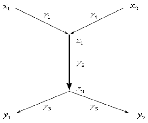
Figure 3. A positive exchange value

Now, let

$$\tilde{q}=\bar{q}+\left(\begin{array}[]{cc}-\epsilon&\epsilon\\ \epsilon&-\epsilon\end{array}\right),$$

where $\epsilon$ is a sufficiently small positive number. Then, by (3.22),

$$g\cdot\tilde{q} = g\cdot\left(\bar{q}+\left(\begin{array}[]{cc}-\epsilon&\epsilon\\ \epsilon&-\epsilon\end{array}\right)\right)$$

$$= g\cdot\bar{q}+\epsilon\left(-g_{11}+g_{12}+g_{21}-g_{22}\right)=g\cdot\bar{q},$$

which shows that $\tilde{q}$ is compatible with $G$. Now, we show $u_{1}\left(\tilde{q}_{1}\right)>u_{1}\left(\bar{q}_{1}\right)$. Since $\bar{q}_{1}=\left(\bar{q}_{11},\bar{q}_{21}\right)\in\mathbb{R}_{++}^{2}$ is derived from the utility maximization problem (2.2) of consumer $1,$ it must satisfy the first order condition at $\bar{q}_{1}$:

(3.24) $$\partial u_{1}\left(\bar{q}_{1}\right)/\partial q_{1}=\lambda p_{11}\text{ and }\partial u_{1}\left(\bar{q}_{1}\right)/\partial q_{2}=\lambda p_{21}$$

for some $\lambda>0$. Thus, using Taylor’s Theorem, we have

$$u_{1}\left(\tilde{q}_{1}\right) = u_{1}\left(\bar{q}_{1}\right)+\frac{\partial u_{1}\left(\bar{q}_{1}\right)}{\partial q_{11}}\left(\tilde{q}_{11}-\bar{q}_{11}\right)+\frac{\partial u_{1}\left(\bar{q}_{1}\right)}{\partial q_{21}}\left(\tilde{q}_{21}-\bar{q}_{21}\right)+o\left(\epsilon\right)$$

$$= u_{1}\left(\bar{q}_{1}\right)+\lambda p_{11}\left(-\epsilon\right)+\lambda p_{21}\epsilon+o\left(\epsilon\right)\text{, by (\ref{FOC1})}$$

$$= u_{1}\left(\bar{q}_{1}\right)+\lambda\epsilon\left(p_{21}-p_{11}\right)+o\left(\epsilon\right)$$

$$> u_{1}\left(\bar{q}_{1}\right)\text{, by (\ref{price_condition}).}$$

Similarly, we have $u_{2}\left(\tilde{q}_{2}\right)>u_{2}\left(\bar{q}_{2}\right)$. This shows that $\tilde{q}\in\mathcal{F}_{G}$. By Lemma 2.1, we have $S\left(\tilde{q}\right)>S\left(\bar{q}\right)$, and thus

$$\mathcal{V}\left(G\right)=\underset{q\in\mathcal{F}_{G}}{\max}\text{ }S\left(q\right)-S\left(\bar{q}\right)\geq S\left(\tilde{q}\right)-S\left(\bar{q}\right)>0.$$

∎

Theorem 3.2.

Suppose $u_{j}$ is differentiable at $\bar{q}$ with $\nabla u_{j}\left(\bar{q}_{j}\right)\in\mathbb{R}_{++}^{k},$ $j=1,...,\ell,$ and $\bar{q}\in\mathbb{R}_{++}^{k\ell}.$ If there exists some $i_{1}\neq i_{2}\in\left\{1,...,k\right\}$, $j_{1}\neq j_{2}\in\left\{1,...,\ell\right\}$ satisfies

$$p_{i_{2}j_{1}}>p_{i_{1}j_{1}},p_{i_{1}j_{2}}>p_{i_{2}j_{2}}\text{ and }V\left(g_{i_{1}j_{2}}\right)\cap V\left(g_{i_{2}j_{1}}\right)\neq\emptyset$$

for $G\in\Omega\left(\bar{q}\right)$, then $\mathcal{V}\left(G\right)>0$.

Proof.

This follows from an analogous proof of proposition 3.9, as shown in Figure 4. ∎

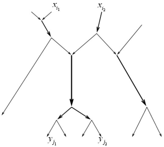
Figure 4. A ramified transport system with positive exchange value.

To conclude this section, we’ve seen how transport structures, preferences and prices jointly determine the exchange values. Each of these factors may lead to a zero exchange value under very rare situations. More precisely, when the structure of the transport system yields a singleton feasible set $\mathcal{F}_{G}$ (Corollary 3.1, Proposition 3.3), or the utility functions are merely quantity dependent (Proposition 3.5), or price vectors are collinear across consumers (Proposition 3.8), the exchange value is zero. However, under more regular situations, there exists a positive exchange value for a ramified transport system. For instance, if the utility functions satisfy the conditions in (3) of Theorem 3.1 with a non-singleton feasible set $\mathcal{F}_{G}$ (Theorem 3.1) or the transport systems are of ramified structures with some non collinear price vectors (Theorem 3.2), there exists a positive exchange value.

4. A New Optimal Transport Problem

In the previous section, we have considered the exchange value $\mathcal{V}\left(G\right)$ for any $G\in\Omega\left(\bar{q}\right)$. A natural question would be whether there exists a $G^{\ast}$ that maximizes $\mathcal{V}\left(G\right)$ among all $G\in\Omega\left(\bar{q}\right)$. The answer to this question has already been provided in Proposition 3.1 as the particular transport path $\bar{G}\in\Omega\left(\bar{q}\right)$ is an obvious maximizer. However, despite the fact that $\bar{G}$ maximizes exchange value, it may be inefficient when accounting for transportation cost. Nevertheless, as indicated previously, one should not neglect the benefit of obtaining an exchange value from a transport system. As a result, it is reasonable to consider both transportation cost and exchange value together when designing a transport system.

Recall that in [33] etc, a ramified transport system is modeled by a transport path between two probability measures $\mathbf{a}$ and $\mathbf{b}$. For each transport path $G\in Path\left(\mathbf{a,b}\right)$ and any $\alpha\in\left[0,1\right]$, the $\mathbf{M}_{\alpha}$ cost of $G$ is defined by

(4.1) $$\mathbf{M}_{\alpha}\left(G\right):=\sum_{e\in E\left(G\right)}w\left(e\right)^{\alpha}length\left(e\right).$$

When $\alpha<1$, a “Y-shaped” path from two sources to one target is usually more preferable than a “V-shaped” path. In general, a transport path with a branching structure may be more cost efficient than the one with a “linear” structure. A transport path $G\in Path\left(\mathbf{a,b}\right)$ is called an $\alpha-$optimal transport path if it is an $\mathbf{M}_{\alpha}$ minimizer in $Path\left(\mathbf{a,b}\right)$.

Based on the above discussions, we propose the following minimization problem.

Problem 4.1.

Given two atomic probability measures $\mathbf{a}$ and $\mathbf{b}$ on $X$ in an economy $\mathcal{E}$ given by (2.1), find a minimizer of

(4.2) $$H_{\alpha,\sigma}\left(G\right):=M_{\alpha}\left(G\right)-\sigma\mathcal{V}\left(G\right)$$

among all $G\in\Omega\left(\bar{q}\right)$, where $\Omega\left(\bar{q}\right)$ is given by (3.2), and $\alpha\in[0,1)$ and $\sigma\geq 0$ are fixed constants.

When the utility functions are merely quantity dependent (Proposition 3.5) or when price vectors are collinear across consumers (Proposition 3.8), the exchange value of any $G\in\Omega\left(\bar{q}\right)$ is always zero. In these cases, $H_{\alpha,\sigma}\left(G\right)=M_{\alpha}\left(G\right)$ for any $\sigma$. Thus, the study of $H_{\alpha,\sigma}$ coincides with that of $M_{\alpha}$, which can be found in existing literature (e.g. [33], [7]). However, as seen in the previous section, it is quite possible that $H_{\alpha,\sigma}$ does not agree with $M_{\alpha}$ on $\Omega\left(\bar{q}\right)$ for $\sigma>0$ in a general economy $\mathcal{E}$.

As $\mathcal{V}$ is topologically invariant (Proposition 3.4), many results that can be found in literature about $M_{\alpha}$ still hold for $H_{\alpha,\sigma}$. For instance, the Melzak algorithm for finding an $M_{\alpha}$ minimizer ([28], [19], [7]) in a fixed topological class still applies to $H_{\alpha,\sigma}$ because $\mathcal{V}\left(G\right)$ is simply a constant within each topological class. Also, as the balance equation (2.6) still holds, one can still calculate angles between edges at each vertex using existing formulas ([33]), and then get a universal upper bound on the degree of vertices on an optimal $H_{\alpha,\sigma}$ path.

However, due to the existence of exchange value, one may possibly favor an optimal $H_{\alpha,\sigma}$ path instead of the usual optimal $M_{\alpha}$ path when designing a transport system. The topological type of the optimal $H_{\alpha,\sigma}$ path may differ from that of the optimal $M_{\alpha}$ path. This observation is illustrated by the following example.

(a) $G_{1}$

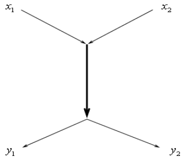
(b) $G_{2}$

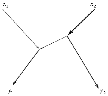
(c) $G_{3}$

Figure 5. Three topologically different transport systems.

Example 4.1.

Let us consider the transportation from two sources to two consumers. If we only consider minimizing $\mathbf{M}_{\alpha}$ transportation cost, each of the three topologically different types shown in Figure 5 may occur. However, when $\sigma$ is sufficiently large, only $G_{2}$ in Figure 5b may be selected under suitable conditions of $u$ and $p$. This is because $G_{2}$ has a positive exchange value which does not exist in either $G_{1}$ or $G_{3}$.

References

- [1] L. Ambrosio. Lecture notes on optimal transport problems. Mathematical aspects of evolving interfaces (Funchal, 2000), 1–52, Lecture Notes in Math., 1812, Springer, Berlin, 2003.
- [2] K. Arrow. and F. Hahn. General Equilibrium Analysis. San Francisco: Holden-Day, 1971.
- [3] Y. Brenier. Décomposition polaire et réarrangement monotone des champs de vecteurs. C. R. Acad. Sci. Paris Sér. I Math. 305 (1987), no. 19, 805–808.
- [4] L.A. Caffarelli; M. Feldman; R. J. McCann. Constructing optimal maps for Monge’s transport problem as a limit of strictly convex costs. J. Amer. Math. Soc. 15 (2002), no. 1, 1–26
- [5] A. Brancolini, G. Buttazzo, F. Santambrogio, Path functions over Wasserstein spaces. J. Eur. Math. Soc. Vol. 8, No.3 (2006),415–434.
- [6] M. Bernot; V. Caselles; J. Morel, Traffic plans. Publ. Mat. 49 (2005), no. 2, 417–451.
- [7] M. Bernot; V. Caselles; J. Morel; Optimal Transportation Networks: Models and Theory. Series: Lecture Notes in Mathematics , Vol. 1955 , (2009).
- [8] G. Buttazzo and G. Carlier. Optimal spatial pricing strategies with transportation costs. To appear in Contemp. Math..
- [9] J. Chipman and J. Moore. Compensating Variation, Consumer’s Surplus, and Welfare. American Economic Review, Vol 70, No. 5, 1980, 933-949.
- [10] T. De Pauw and R. Hardt. Size minimization and approximating problems, Calc. Var. Partial Differential Equations 17 (2003), 405-442.
- [11] G. Devillanova and S. Solimini. On the dimension of an irrigable measure. Rend. Semin. Mat. Univ. Padova 117 (2007), 1–49.
- [12] G. Debreu. The Coefficient of Resource Utilization, Econometrica, Vol. 19, No. 3, 1951, 273-292.
- [13] G. Debreu. Theory of Value. Wiley, New York, 1959.
- [14] J. Eaton and S. Kortum. Technology, Geography, and Trade, Econometrica, Vol. 70, No. 5, 2002, 1741-1779.
- [15] L.C. Evans and R. Gariepy. Measure theory and fine properites of functions. Stud. Adv. M ath., CRC Press, 1992
- [16] L. C. Evans; W. Gangbo. Differential equations methods for the Monge-Kantorovich mass transfer problem. Mem. Amer. Math. Soc. 137 (1999), no. 653.
- [17] A. Figalli, Y.H. Kim and R.J. McCann. When is multidimensional screening a convex program? Preprint (2010).
- [18] W. Gangbo; R. J. McCann. The geometry of optimal transportation. Acta Math. 177 (1996), no. 2, 113–161.
- [19] E.N. Gilbert. Minimum cost communication networks, Bell System Tech. J. 46, (1967), pp. 2209-2227.
- [20] R. Jordan, D. Kinderlehrer and F. Otto. The variational formulation of the Fokker-Planck equation. SIAM J. Math. Anal. 29,1 (1998), 1-17.
- [21] L. Kantorovich. On the translocation of masses. C.R. (Doklady) Acad. Sci. URSS (N.S.), 37:199-201, 1942.
- [22] T. Koopmans. Three Essays on the State of Economic Science, McGraw-Hill, New York, 1957.
- [23] O. Lange. The Foundation of Welfare Economics, Econometrica, Vol. 10, No. 3/4, 1942, 215-228.
- [24] X. Ma, N. Trudinger, and X.J. Wang. Regularity of potential functions of the optimal transportation problem. Arch. Rat. Mech. Anal., 177(2005), 151-183.
- [25] F. Maddalena, S. Solimini and J.M. Morel. A variational model of irrigation patterns, Interfaces and Free Boundaries, Volume 5, Issue 4, (2003), pp. 391-416.
- [26] G. Monge. Mémoire sur la théorie des déblais et de remblais, Histoire de l’Académie Royale des Sciences de Paris, avec les Mémorires de Mathématique et de Physique pour la même année, pages 666-704 (1781).
- [27] A. Mas-Colell, M. Whinston and J. Green. Microeconomic Theory, Oxford University Press, New York, 1995.
- [28] Z.A. Melzak. On the problem of Steiner, Canad. Math. Bull. 4 (1961) 143-148.
- [29] E. Paolini and E. Stepanov. Optimal transportation networks as flat chains. Interfaces and Free Boundaries, 8 (2006), 393-436.
- [30] P. Samuelson. Foundations of Economic Analysis. Harvard University Press, Cambridge, 1947.
- [31] C. Villani. Topics in mass transportation. AMS Graduate Studies in Math. 58 (2003).
- [32] B. White. Rectifiability of flat chains. Annals of Mathematics 150 (1999), no. 1, 165-184.
- [33] Q. Xia. Optimal paths related to transport problems. Communications in Contemporary Mathematics. Vol. 5, No. 2 (2003) 251-279.
- [34] Q. Xia. Interior regularity of optimal transport paths. Calculus of Variations and Partial Differential Equations. 20 (2004), no. 3, 283–299.
- [35] Q. Xia. Boundary regularity of optimal transport paths. Preprint.
- [36] Q. Xia. The formation of tree leaf. ESAIM Control Optim. Calc. Var. 13 (2007), no. 2, 359–377.
- [37] Q. Xia. The geodesic problem in quasimetric spaces. Journal of Geometric Analysis. Volume 19, Issue2 (2009), 452–479.
- [38] Q. Xia and A. Vershynina. On the transport dimension of measures. SIAM J. Math. Anal. Volume 41, Issue 6, pp. 2407-2430 (2010).
- [39] G. Xue, T. Lillys and D. Dougherty. Computing the Minimum Cost Pipe Network Interconnecting One Sink and Many Sources. SIAM Journal on Optimization. Volume 10 , Issue 1 (1999) Pages: 22 - 42 .
- [40] Zhang and Zhu. A bilevel programming method for pipe network optimization. SIAM Journal on Optimization, Vol 6, 838 (1996).