Efficient implementation of bipartite nonlocal unitary gates using prior entanglement and classical communication

Abstract

Any bipartite nonlocal unitary operation can be carried out by teleporting a quantum state from one party to the other, performing the unitary gate locally, and teleporting a state back again. This paper investigates unitaries which can be carried out using less prior entanglement and classical communication than are needed for teleportation. Large families of such unitaries are constructed using (projective) representations of finite groups. Among the tools employed are: a diagrammatic approach for representing entangled states, a theorem on the necessary absence of information at certain times and locations, and a representation of bipartite unitaries based on a group Fourier transform.

I Introduction

Teleportation Bennett_tele makes possible a wide variety of nonlocal quantum processes provided sufficient prior entanglement and classical communication are available. To change the quantum state of two systems $A$ and $B$ separated in space it is only necessary to teleport the $A$ state to the laboratory where $B$ is located, carry out the desired operation, and teleport the result back again. The present paper is concerned with certain types of operations, nonlocal unitaries, which can be achieved at lower cost, in particular less prior entanglement than is needed for two-way teleportation.

Protocols of this sort for qubits were developed by Eisert et al. Eisert and Reznik et al. ReznikNLU , and our work builds upon theirs. See Gottesman ; Chefles ; Chefles2 ; Song ; Huang ; Chen ; OLeary ; Zeng ; Berry ; Dang ; Zhao ; Jang ; Groisman_nonMES ; Cirac ; Dur ; Ye for other deterministic and probabilistic protocols. We only consider the deterministic case in which the desired unitary is carried out with probability 1; finding efficient protocols that allow for some noise is a challenging problem not addressed here. While our protocols can be applied to an arbitrary nonlocal unitary, only in special cases are they more efficient than teleportation.

There are two separate motivations behind studies of the sort presented here. First, it seems likely that nonlocal operations will play a significant role in future quantum computers, especially schemes for distributed computation Cirac_dist ; Yims ; Yims2 ; Meter , and achieving them using prior entanglement is an option that deserves consideration. Since producing entanglement is likely to be expensive, there is an obvious advantage to protocols which use as little of it as possible. By comparison, classical communication is usually thought of as cheap, since it does not have to be protected from decoherence. However, protocols that minimize its use might still have an advantage over those that require more.

A second motivation is the desire to better understand the role of different types of quantum information RBGtypes in various information-processing tasks. General nonlocal unitaries require physical influences to propagate from one side to the other, in fact in both directions, and one would like to understand these in rational terms rather than by invoking quasimagical “collapses” and the like. It turns out that unitary operations place particularly stringent conditions on the presence or absence of different types of information at different locations and different times throughout a protocol, and knowing what these are can provide insight into why certain gates and measurements need to be employed rather than others. In this respect our analysis represents an advance over earlier work.

Our protocols are based upon expanding a nonlocal unitary on ${\cal H}_{A}\otimes{\cal H}_{B}$ in the form

$${\cal U}=\sum_{j=1}^{N}A_{j}\otimes B_{j},$$ (1)

where the Hilbert spaces ${\cal H}_{A}$, ${\cal H}_{B}$ have finite dimensions $d_{A},d_{B}$ respectively, the $A_{j}$ operators satisfy special conditions, or are of a particular type, and the expansion coefficients $B_{j}$, obviously constrained by the requirement that ${\cal U}$ be unitary, may have additional special properties. In the simplest situation of “controlled” unitaries, the one easiest to understand in information-theoretic terms, the $A_{j}$ form a projective decomposition of the identity on ${\cal H}_{A}$, and the $B_{j}$ are arbitrary unitaries on ${\cal H}_{B}$. A more complex, but also more general case is unitaries of “group” form (or “group-unitaries”), when the $A_{j}$ are unitary operators that form a representation, possibly a projective representation, of a group $G$, and the sum in (1) is a sum over elements in this group. Here the $B_{j}$ may also be proportional to unitary operators forming a (projective) representation of the same group $G$, but that is not a requirement of our protocol. Actually any bipartite unitary can be written in this form with some suitable choice of the group $G$, thus the term “group-unitaries” should be regarded as describing the form of expansion of ${\cal U}$, rather than a property of ${\cal U}$ itself. There is some relationship between our use of groups for nonlocal unitaries and the protocol of Klappenecker et al. Klappenecker for implementing local unitary gates.

The remainder of this paper is organized as follows: Sec. II indicates the general strategy for our protocols, shows through a diagrammatic approach why groups are useful, establishes an information theorem that is useful when discussing unitaries, and a lower bound on how much entanglement is needed.

The discussion of particular protocols begins in Sec. III with controlled unitaries that generalize Eisert and are easily understood in information-theoretic terms. The presentation of the main group-unitary protocol in Sec. IV begins with a general definition and a quantum circuit, followed by a detailed analysis in Sec. IV.2 of why the protocol works. A procedure related to group Fourier transforms is used in Sec. IV.3 to give a general parametrization of unitaries which can be realized in this fashion. A particular case in which the $A$ and $B$ systems are treated in a symmetrical fashion is the subject of Sec. IV.4, and in Sec. IV.5 it is shown that the controlled unitaries of Sec. III can be rewritten in the group form in an efficient way.

Several specific examples of nonlocal unitaries are presented in Sec. V. This is followed by a summary of the paper in Sec. VI, which notes some issues deserving further study. The appendices contain proofs and other subsidiary material.

II General Comments

II.1 Overall structure of protocols

The protocols discussed in this paper all have a common structure indicated schematically in Fig. 1. The two parties share an entangled state on ancillary systems $a$ and $b$. Alice performs a unitary gate $T$ on systems $a$ and $A$, followed by a measurement of the $a$ system. She sends the (classical) measurement result to Bob, who uses this to determine which unitary $U$ to carry out on $b$ and $B$. Bob then measures the $b$ system and sends the result back to Alice, who uses this information to choose a unitary $V$ carried out on $A$. It is worth noting that the straightforward teleportation protocol mentioned in Sec. I can also be represented using Fig. 1 provided the initial entangled resource is large enough to allow teleportation in both directions. (We leave as an exercise to the reader working out the details of the unitaries $T$, $U$ and $V$ needed to achieve this.) Such protocols are inherently asymmetric in that one party has to take the first step, while the second party acts according to the information received from the first party.

Figure 1: A prototypical circuit diagram for local implementation of nonlocal unitaries

II.2 Why groups are useful

Our most powerful protocols are based on expansions of the desired nonlocal unitary ${\cal U}$ in terms of a matrix representation of a finite group. Indeed, all unitaries can be expanded in this way. Here, we explain why groups are useful utilizing an intuitive and visual presentation involving diagrams Cohen_tele ; Cohen_UPB , from which as an additional benefit we will gain insight into one of our most important contributions, that unlike in previously published protocols, the Schmidt rank $N$ of the entangled resource can be chosen independently of the dimensions $d_{A},d_{B}$ of Hilbert spaces ${\cal H}_{A},~{}{\cal H}_{B}$ on which ${\cal U}$ acts. We note that it was by using these diagrams that we discovered the first of our protocols, which uses a uniformly entangled state to implement unitaries of the form

$${\cal U}=\sum_{j=0}^{N-1}c(j)U(j)\otimes V(j),$$ (2)

with $\{U(j)\},\,\{V(j)\}$ two sets of unitaries, and the operators $U(j)\otimes V(j)$ form an ordinary representation of a group. All other protocols based on groups were then discovered as generalizations of this one.

The idea underlying our diagrams is that the presence of entanglement on systems $a,b$ effectively creates multiple images of the states of other systems, in our case, $A$ and $B$ (see Cohen_tele ; Cohen_UPB for detailed discussion of these ideas). That is, the state

$$|\Phi\rangle\otimes|\Psi\rangle\propto\left(\sum_{j=0}^{N-1}|j\rangle_{a}|j\rangle_{b}\right)\otimes|\Psi\rangle,$$ (3)

with $|\Phi\rangle$ on systems $a,b$ and $|\Psi\rangle$ on $A,B$, can be represented by the diagram shown in Fig. 2.

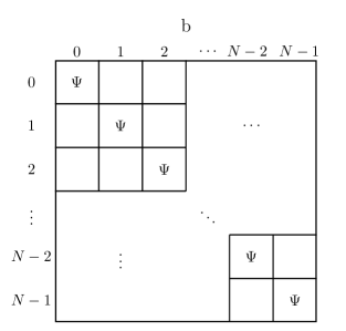
Figure 2: Box diagram illustrating how entanglement creates multiple images of the state $|\Psi\rangle$ distributed along the diagonal of the box.

Figure 3: Result of projection onto the state $|+\rangle_{a}$ following their respective controlled unitaries.

Given the way these images are distributed through the diagram, it is clear that Alice and Bob independently have “access” to each of the individual images, and by performing controlled unitaries, $\sum_{j=0}^{N-1}|j\rangle_{a}\langle j|\otimes U(j)$ and $\sum_{j=0}^{N-1}|j\rangle_{b}\langle j|\otimes V(j)$, on each side, can together attach to each image one of the operators appearing in the terms of the sum for ${\cal U}$ in (2). What we ultimately want is a particular linear combination of all these terms. To see how to accomplish this, note that a measurement on $a$ with outcome $j$ picks out a single row of the diagram, and thus a single image. On the other hand, a measurement outcome $|+\rangle_{a}=\sum_{j=0}^{N-1}|j\rangle_{a}$, places a sum of all the rows into a single row, which will appear as in Fig. 3 (all other rows disappearing), with each column containing one of the terms $|\Psi_{j}\rangle=(U(j)\otimes V(j))|\Psi\rangle$. Similarly, if Alice measures $a$ in the Fourier basis (or equivalently, performs a discrete Fourier transform on $a$ and then measures in the standard basis), then for any outcome the diagram is collapsed into a single row, with each column containing one of the terms $|\Psi_{j}\rangle$ multiplied by a phase factor. These phase factors, $e^{i\xi_{j}}$, can easily be removed by Bob performing $\sum_{j=0}^{N-1}e^{-i\xi_{j}}|j\rangle_{b}\langle j|$ on system $b$ leaving, for all outcomes of Alice’s measurement on $a$, the diagram in Fig. 3.

The next step is for Bob to make a measurement of his own on system $b$, designed to place the factors $c(j)$ on the appropriate images and to take linear sums of these terms, collapsing the diagram finally into a single small box. If he first performs a unitary $C$, the first row of which is given by $\sum_{j=0}^{N-1}c(j)|0\rangle_{b}\langle j|$, and then measures in the standard basis with outcome corresponding to state $|0\rangle_{b}$, the result will be precisely the desired unitary operation,

$${\cal U}|\Psi\rangle=\sum_{j=0}^{N-1}c(j)|\Psi_{j}\rangle.$$ (4)

The question is how to complete this unitary, $C$. Clearly, we cannot simply copy the first row into all the others, as the rows of a unitary matrix must all be mutually orthogonal, even though this would produce (4) for every outcome of Bob’s subsequent measurement. One possibility that turns out will always work (see Sec. IV.4) is to choose all the other rows of $C$ as permutations of its first row. This choice does not automatically yield (4), however, but we instead obtain

$${\cal U}^{\prime}|\Psi\rangle=\sum_{j=0}^{N-1}c(\Pi(j))|\Psi_{j}\rangle,$$ (5)

where $\Pi(j)$ represents the permutation for the given outcome and ${\cal U}^{\prime}\neq{\cal U}$, implying that our protocol has failed unless we can find a way to correct it. Such a correction is certainly possible if there exist local unitaries on ${\cal H}_{A},{\cal H}_{B}$ that together transform $|\Psi_{j}\rangle$ to $|\Psi_{\Pi(j)}\rangle$, and hence ${\cal U}^{\prime}$ into ${\cal U}$. This is where the notion of groups enters the picture. Indeed, recalling that $|\Psi_{j}\rangle=\left(U(j)\otimes V(j)\right)|\Psi\rangle$, then if Alice and Bob perform $U(k)\otimes V(k)$, and can choose $k$ such that $U(k)U(j)=U(\Pi(j))$ and $V(k)V(j)=V(\Pi(j))$ with $\Pi(j)$ corresponding to the multiplication table of a group $G$, then this transforms ${\cal U}^{\prime}$ into ${\cal U}$ and we have successfully, and deterministically, implemented ${\cal U}$. See Sec. IV.4 for further details. Note that the requirement expressed in the previous discussion is that $U,V$ each form a representation of the group $G$. One could consider the possibility that they are non-unitary representations, but the corrections just described would then not generally be possible deterministically. Therefore, we consider only unitary representations in the sequel.

Finally, we note that it should be clear from this discussion that $N$ can be chosen as a completely independent quantity; in particular, there is no reason for it to be constrained by the values of $d_{A}$ or $d_{B}$, as has been the case in previously known protocols. Hence, the amount of entanglement needed to implement a given nonlocal unitary depends only on the form of the unitary itself—in particular for our protocols, on the possible ways it can be expanded in terms of a group—and not on the size of the local Hilbert spaces upon which it acts.

II.3 Information location

To understand various aspects of our protocols, it will be useful to “quantize” the circuit in Fig. 1, by replacing measurements and classical communication with appropriate controlled unitaries, Fig. 4. An easy way of seeing the equivalence of the two circuits in terms of their action on systems $A$ and $B$ is to imagine that the ancillary systems in Fig. 4 are measured in the standard basis at a time corresponding to the right side of the diagram. Then using the fact that quantum measurements reveal pre-existing properties when one employs an appropriate framework note_framework , one can infer that systems $a$ and $b$ were in the states indicated by these outcomes, $|l\rangle$ and $|m\rangle$ respectively, before the measurements took place and thus also at times preceding the controlled operations, i.e., at the times when the measurements in Fig. 1 took place.

Figure 4: Quantized version of Fig. 1.

While Figs. 1 and 4 are equivalent so far as $A$ and $B$ are concerned, the latter is simpler to analyze in terms of certain information-theoretical ideas by using the following theorem.

Theorem 1.

If ${\cal J}$ is an isometry mapping a Hilbert space ${\cal H}_{R}$ to a tensor product ${\cal H}_{R}\otimes{\cal H}_{S}$, the following statements are equivalent:

(i) ${\cal J}$ generates a unitary from ${\cal H}_{R}$ to itself in the sense that

$${\cal J}|r\rangle=({\cal U}|r\rangle)\otimes|s_{0}\rangle,$$ (6)

with ${\cal U}:{\cal H}_{A}\rightarrow{\cal H}_{A}$ a unitary operator and $|s_{0}\rangle$ a fixed state (independent of $|r\rangle$) in ${\cal H}_{S}$.

(ii) There is no information about the initial state of $R$ available in $S$ after applying ${\cal J}$.

(iii) The Kraus operators $\{K_{j}\}$ such that

$${\cal J}|r\rangle=\sum_{j}K_{j}|r\rangle\otimes|s_{j}\rangle,$$ (7)

for $\{|s_{j}\rangle\}$ some orthonormal basis of ${\cal H}_{S}$, are of the form $K_{j}=c_{j}{\cal W}$, with the $c_{j}$ complex numbers and ${\cal W}$ a map from ${\cal H}_{R}$ to itself.

By “no information” we mean that the final state of $S$ is uncorrelated with the initial state of $R$, see RBG05 , and thus no conceivable measurement on $S$ will yield any information about the initial state of $R$. It is then obvious that (i) implies (ii) and (iii); the reverse inferences are proved in Appendix A.

To apply this theorem to the situation in Fig. 4 let ${\cal V}$ be the unitary represented by this quantum circuit, $|r\rangle$ the initial state of the combined $A$ and $B$ system thought of as $R$, $|\Phi\rangle$ the (fixed) initial state of $a$ and $b$, which together constitute the system $S$, and

$${\cal J}|r\rangle:={\cal V}(|r\rangle\otimes|\Phi\rangle).$$ (8)

The theorem then tells us that if the circuit carries out a unitary ${\cal U}$ on ${\cal H}_{A}\otimes{\cal H}_{B}$ it must be the case that no information about the initial state of $AB$ can be found in the final state of the combined ancillary systems $a$ and $b$, and therefore none is present in either $a$ or $b$ at a time after the controlled gate that represents its final interaction with the rest of the system. We will see in Sec. III how this absence of information can be used to motivate the choice of certain parts of a circuit to carry out nonlocal unitaries. Of course at a time before the final controlled interactions, the ancillary systems are (in general) correlated with, and thus contain information about, the rest of the system; it is only after the final interactions, the choice of which is constrained by the need to remove this information from the ancillas, that they are in an appropriate sense of the term “information-free”. Since the measurement outcomes in Fig. 1 are exactly the same as if the measurements were carried out at the end of the time interval shown in Fig. 4, we see that such outcomes cannot contain any information about the input $AB$. On the other hand, there certainly exist measurements that Alice could carry out on $a$ that would indeed reveal information about the input state of $AB$, and in that case we cannot implement deterministically a unitary ${\cal U}$ on ${\cal H}_{A}\otimes{\cal H}_{B}$. Conversely, if there is no information about the $AB$ input in the final state of the ancillaries, then the circuit in Fig. 4, and hence its counterpart in Fig. 1, will necessarily result in a unitary map of the $AB$ input to the $AB$ output.

Statement (iii) of the theorem provides an alternative way of deciding if a circuit implements a unitary on $R$. Suppose the whole circuit is (or is equivalent to) a unitary followed by a measurement in an orthonormal basis of ${\cal H}_{S}$. If for every measurement outcome the corresponding Kraus operator on $R$ is proportional to the same operator, then the circuit deterministically implements a unitary on $R$. Checking this may be easier than working out the entire state evolution for an arbitrary initial state of $R$.

II.4 Bounds on resources

The theorem that follows provides a very general lower bound on the amount of entanglement resource needed to implement a nonlocal unitary. By the Schmidt rank (sometimes called “Schmidt number”) opSchmidt of a bipartite operator on ${\cal H}_{A}\otimes{\cal H}_{B}$ we mean the minimum number of terms in an expansion of the operator as a sum of products of operators on the separate systems, or, equivalently, the rank of the matrix of coefficients $c_{ij}$ when the operator is expanded in the form $\sum_{ij}c_{ij}A_{i}\otimes B_{j}$ with $\{A_{i}\}$ and $\{B_{j}\}$ bases for the operators on ${\cal H}_{A}$ and ${\cal H}_{B}$. Either definition has an obvious counterpart in the Schmidt rank of a bipartite pure state. There are various ways of defining the “entanglement” of a bipartite unitary operator. For our purposes a useful one is the entangling strength Nielsen of the unitary ${\cal U}_{AB}$ defined as the maximum entanglement of a state on ${\cal H}_{A\bar{A}}\otimes{\cal H}_{B\bar{B}}$ produced by letting ${\cal U}_{AB}\otimes I_{\bar{A}}\otimes I_{\bar{B}}$ act on a product state $|\sigma\rangle_{A\bar{A}}\otimes|\tau\rangle_{B\bar{B}}$, where $\bar{A}$ and $\bar{B}$ are ancillary systems, and $|\sigma\rangle_{A\bar{A}}$ and $|\tau\rangle_{B\bar{B}}$ are arbitrary entangled states. By the entanglement of a pure state we mean the usual measure $-\sum\lambda_{j}\log\lambda_{j}$ in terms of its (squared) Schmidt coefficients $\lambda_{j}$.

Theorem 2.

To generate a bipartite nonlocal unitary ${\cal U}$ using an entangled resource $|\Phi\rangle$ and separable quantum operations Bennett_sep , which include local operations and classical communication (LOCC), the Schmidt rank of $|\Phi\rangle$ cannot be less than the Schmidt rank of ${\cal U}$, and the entanglement of $|\Phi\rangle$ cannot be less than the entangling strength of ${\cal U}$ as defined previously.

The proof will be found in Appendix B. The second assertion remains true if “entanglement” and “entangling strength” both refer to some other entanglement monotone Vidal_ent .

The idea behind the second part of Theorem 2 is that entanglement cannot increase on average under LOCC. Using the same idea, the entanglement that a bipartite unitary can generate for any particular input product state provides a lower bound for the entanglement needed to implement this unitary. The entanglement that unitaries of the form (2) can generate for the input product state $|0\rangle_{A}\otimes|0\rangle_{B}$ has effectively been studied in Hamma .

III Implementing Controlled Unitaries

Figure 5: $Z$-information protocol when $P_{j}$ in (9) projects onto $|j\rangle_{A}$. The $j$ label appears twice, reflecting the fact that the $Z$ type of information about system $A$ is transmitted to system $b$.

Figure 6: Quantized upper left part of Fig. 5, and an effectively equivalent diagram.

In this section we consider bipartite controlled unitaries of the form

$${{\cal U}}=\sum_{j=0}^{N-1}P_{j}\otimes V_{j},$$ (9)

where the $P_{j}$’s form a (projective) decomposition of the identity on ${\cal H}_{A}$, while the $V_{j}$’s are arbitrary unitaries on ${\cal H}_{B}$. All the essential ideas can be understood assuming the $P_{j}$’s are of rank 1 (i.e., onto pure states) and this is assumed in the exposition that follows, with some remarks toward the end about the extension to a more general situation [see the material associated with (16)].

III.1 Description of the protocol with rank-1 projectors $P_{j}$

Let ${\cal H}_{A}$ be of dimension $N$ and $P_{j}$ a projector onto $|j\rangle$ in the standard basis. Then the circuit in Fig. 5 represents a straightforward generalization of the $N=2$ protocol of Eisert to arbitrary $N$. The entangled resource is

$$|\Phi\rangle_{ab}=\frac{1}{\sqrt{N}}\sum_{k=0}^{N-1}|k\rangle\otimes|k\rangle.$$ (10)

For general $N$ define the $X$ and $Z$ gates using

$$X|k\rangle=|k-1\rangle;\quad Z|k\rangle=e^{2\pi ik/N}|k\rangle,$$ (11)

with subtraction understood as mod $N$, so one has the usual Pauli operators when $N=2$. The first controlled-$X^{j}$ gate in the figure means that if ${\cal H}_{A}$ is in the state $|j\rangle$, then $X^{j}$, meaning $X$ to the power $j$, is applied to the $a$ system. Then Alice performs a measurement on $a$ in the standard basis, and sends the result $l$ to Bob, who applies $X^{l}$ to $b$. This is followed by a controlled-$V$ gate, (9) with $b$ replacing $A$ as the control, on $b$ and $B$. Then comes a Fourier transform

$$F=\frac{1}{\sqrt{N}}\sum_{mj}e^{2\pi imj/N}|m\rangle\langle j|,$$ (12)

on $b$, and a measurement of $b$ in the standard basis. The outcome $m$ is sent to Alice who carries out a $Z_{m}=Z^{-m}$ correction, where $Z$ is defined in (11). [The $F$ gate could be other than (12); see the discussion following (15).] This completes the protocol.

Figure 7: Reduced diagram of the $Z$-information protocol

III.2 Detailed analysis of the circuit

To understand what is accomplished by the upper left part of the circuit in Fig. 5 it is helpful to first quantize it, see the discussion in Sec. II.3, and then show that the quantized version in Fig. 6(a) is effectively the same thing as that in Fig. 6(b). If $A$ is initially in the state $|j\rangle$, unitary time development in Fig. 6(a) involves the two steps (we omit the normalization $1/\sqrt{N}$; note also that $l$ in the figures is equal to $k-j$)

$$|j\rangle\otimes\sum_{k}|k\rangle\otimes|k\rangle\rightarrow|j\rangle\otimes\sum_{k}|k-j\rangle\otimes|k\rangle\rightarrow$$

$$|j\rangle\otimes\Bigl{(}\sum_{k}|k-j\rangle\Bigr{)}\otimes|j\rangle=|j\rangle\otimes\Bigl{(}\sum_{k}|k\rangle\Bigr{)}\otimes|j\rangle.$$ (13)

Thus at the end of these two steps we have a product state on ${\cal H}_{Ab}\otimes{\cal H}_{a}$, with the ${\cal H}_{a}$ part in the state $|+\rangle=\sum_{k}|k\rangle$, independent of $j$. So (ii) of Theorem 1 is satisfied partially: there is no information about $A$ in $a$ at the end of the time interval shown in Fig. 6(a). One might think of the second controlled-$X^{j}$ gate as serving to “erase” the information about $A$ present in $a$ at the intermediate time. Erasing the information makes use of the fact, which justifies the final equality in (13), that addition modulo $N$ is a group, and for any finite group a sum over the group elements $g$ is the same as a sum over $gh$ with $h$ fixed and $gh$ the group product. In Sec. IV below, we employ this strategy using a more general group.

As demonstrated in (13) the net result of the upper left part of the circuit in Fig. 5 is to copy the value of $j$ in $|j\rangle_{A}$ from ${\cal H}_{A}$ to ${\cal H}_{b}$, precisely what one finds in Fig. 6(b). This is the first step in what is sometimes called “one bit teleportation” 1bitTeleport , and amounts to copying a particular type of quantum information, the $Z$ type or its generalization to $N>2$ in the notation of RBGtypes , from $A$ to $b$. The nonlocal operation in Fig. 6(b), an isometry from $A$ to the combined $A$-$b$ system, is what is effectively accomplished by the first steps of the protocol, including the classical communication which is essential for actually transferring the information from Alice’s laboratory to Bob’s. (Note, however, that the information is not contained in the “classical” outcome of the measurement, but resides in correlations between this outcome and system $b$; see the analysis in RBG02 .)

When we replace the upper left part of the circuit in Fig. 5 with Fig. 6(b) and quantize the remainder, the result is Fig. 7, where the unitary time development following the controlled-$V$ gate takes the form, assuming an initial $AB$ state $|j\rangle\otimes|B\rangle$:

$$|j\rangle\otimes|j\rangle\otimes V_{j}|B\rangle\rightarrow\sum_{m}\Bigl{(}\langle m|F|j\rangle\Bigr{)}|j\rangle\otimes|m\rangle\otimes V_{j}|B\rangle$$

$$\rightarrow\sum_{m}\Bigl{(}\langle m|F|j\rangle\Bigr{)}Z_{m}|j\rangle\otimes|m\rangle\otimes V_{j}|B\rangle$$ (14)

For a successful unitary it is necessary, see the discussion in Sec. II.3 following Theorem 1, that the final state in (14) be a product of a pure state on ${\cal H}_{b}$ times another on ${\cal H}_{AB}$. This can be achieved if we assume that

$$Z_{m}|j\rangle=c\langle m|F|j\rangle^{-1}|j\rangle,$$ (15)

since the right hand side of (14) will then be of the desired form $c|j\rangle\otimes\Bigl{(}\sum_{m}|m\rangle\Bigr{)}\otimes V_{j}|B\rangle$. But for $Z_{m}$ in (15) to be a unitary it is necessary and sufficient that the unitary operator $F$ be such that all its matrix elements in the standard basis are of magnitude $1/\sqrt{N}$, and then $|c|=1/\sqrt{N}$ as well. There are many possibilities for such a unitary matrix, but one obvious choice is the Fourier transform in Eq. (12), and then $Z_{m}=Z^{-m}$, with $Z$ defined in (11). Using this or some other appropriate choice for the $F$ and $Z_{m}$ gates will result in a final state, Fig. 7, of $|j\rangle\otimes|+\rangle\otimes V_{j}|B\rangle$, if the initial $AB$ state is $|j\rangle\otimes|B\rangle$. By linearity this extends to any other initial $AB$ state.

III.3 Generalization to projectors $P_{j}$ of higher rank

Minor and fairly obvious changes are all that is needed to extend the discussion from rank 1 to projectors $P_{j}$ of general rank in (9). First, the controlled-$X^{j}$ gates in Figs. 5 and 6, both (a) and (b), should be replaced by the unitary operator

$$\sum_{j}P_{j}\otimes\sum_{k}|k\rangle\langle j+k|,$$ (16)

where the $P_{j}$ act on ${\cal H}_{A}$, a space of any dimension greater than or equal to $N$, and addition is mod $N$. Second, the final $Z_{m}$ gates in Fig. 5 now take the form

$$Z_{m}=\sum_{j}\sqrt{N}\langle m|F|j\rangle^{-1}P_{j}=\sum_{j}e^{-2\pi ijm/N}P_{j}.$$ (17)

where the right side is what results when $F$ is the Fourier transform (12). The argument that this will produce the nonlocal unitary ${\cal U}$ then follows exactly the same steps as before.

The collection of commuting projectors $\{P_{j}\}$ can very well be thought of as representing a certain type of information in the notation of RBGtypes , namely the type that answers the question as to which of these properties, which $j$, is true. Let us refer to this again as “$Z$ information”. Then the generalized protocol functions in essentially the same way as when the $P_{j}$ are of rank 1: The $Z$ information is copied onto the $b$ system by a process that resembles one step in teleportation, here it is used to “choose” which $V_{j}$ is to be carried out, and then erased off the $b$ system by a process which amounts to applying a unitary correction to $A$.

A point worth making, since it will come up again, is that while the success of the protocol, and thus the type of unitary that can be implemented this way, depends upon precise details of the ancillary systems $a$ and $b$, it only depends upon $A$ and $B$ in a more general way: operators on the latter pair of systems must satisfy certain algebraic conditions, but are not otherwise constrained. In the case at hand the operators on ${\cal H}_{A}$ must be a family of commuting projectors that sum to the identity, while on ${\cal H}_{B}$ they must be unitaries. Beyond this there are no requirements, which in particular means that the dimensions of ${\cal H}_{A}$ and ${\cal H}_{B}$ can be arbitrarily large compared to $N$.

IV Protocols Based on a Finite Group

IV.1 Introduction to the group form of unitaries

The protocols discussed in this section are based on the use of a finite group $G$, elements $f$, $g$, and so on, identity $e$, group multiplication indicated by $fg$, in general not equal to $gf$. We shall want to consider cases in which a unitary ${\cal U}$ on a tensor product ${\cal H}_{A}\otimes{\cal H}_{B}$ can be expressed in the form

$${\cal U}=\sum_{f\in G}U(f)\otimes W(f),$$ (18)

where the unitary operators $U(f)$ on ${\cal H}_{A}$ form a finite-dimensional projective representation of $G$ in the sense that for all $f$ and $g$

$$U(f)U(g)=\mu(f,g)U(fg).$$ (19)

Here the $\mu(f,g)$ are nonzero complex numbers constituting a factor system; in our case they are of magnitude 1 because the $U(f)$ are unitary. We shall sometimes have occasion to use (19) in the form

$$U^{\dagger}(g)U(f)=\mu^{\ast}(g,g^{-1}f)U(g^{-1}f),$$ (20)

whose validity can be checked by left multiplying both sides by $U(g)$, the inverse of $U^{\dagger}(g)$, and noting that $\mu^{\ast}(f,g)=1/\mu(f,g)$. As for our purposes it represents no loss of generality, we shall also assume that $U(e)=I_{A}$, and consequently

$$\mu(e,f)=\mu(f,e)=1,\,\,\forall f\in G.$$ (21)

Naturally, an ordinary representation of $G$ in which $\mu(f,g)=1$ for every $f$ and $g$ is one possibility, but we will also consider examples in which the collection $\{U(f)\}$ constitutes a “group up to phases” with nontrivial phases.

Figure 8: Circuit diagram illustrating local implementation of nonlocal unitary ${{\cal U}}=\sum_{f}U(f)\otimes W(f)$, where the set of unitaries $\{U(f)\}$ forms a projective representation of a group.

Figure 8 shows a circuit that will carry out the unitary ${\cal U}$ in (18) with the help of a suitable entangled state, as discussed in detail in Sec. IV.2 below, which gives sufficient conditions on $W(f)$ so the protocol will succeed. The relationship between ${\cal U}$ and the $W(f)$ is analyzed further in Sec. IV.3. A particular case in which each $W(f)$ is proportional to a unitary $V(f)$ representing the same group is the topic of Sec. IV.4, while in Sec. IV.5 we discuss the relationship of the expansion form (18) with the controlled unitaries.

Before proceeding, let us first give a brief description of the circuit of Fig. 8. Alice begins the protocol by implementing a controlled set of unitaries, where system $a$ in standard basis state $|f\rangle_{a}$ controls the unitary $U(f)$, which operates on ${\cal H}_{A}$. She then measures $a$ in a basis unbiased to the standard basis and defined by unitary operator $F$, where by unbiased we mean that when represented in the standard basis, $F$ must have all entries of magnitude $|G|^{-1/2}$. Next, Alice tells Bob the outcome $h$ of that measurement, and he follows by performing diagonal unitary $Z(h)$ on $b$, which has the effect of removing phase factors introduced by Alice’s measurement. He then performs unitary $M$ on $bB$ (defined in (30) and (31) below), which introduces the operators $W(f)$ of (18) in a way that is correlated with the $U(f)$’s of Alice’s earlier operation, where these correlations are made possible by the initial entanglement between $a$ and $b$. Bob then measures $b$ in the standard basis and tells Alice his outcome, $g$. Alice completes the protocol with the “correction” $U(g)^{\dagger}$ on $A$, which adjusts the correlation between $W$’s and $U$’s so that the result is always equal to ${\cal U}$ [that is, so that $W(f)$ is always tensored with $U(f)$, rather than with $U(f^{\prime})$ for some $f^{\prime}\neq f$].

IV.2 Discussion of the circuit

Now let us analyze this protocol in detail to understand how and why it works. In view of linearity it suffices to analyze the circuit in Fig. 8 for a product input state $|A\rangle\otimes|B\rangle$. The resource entangled state is

$$|\Phi\rangle_{ab}=\frac{1}{\sqrt{|G|}}\sum_{f\in G}|f\rangle\otimes|f\rangle,$$ (22)

where the kets represent orthonormal basis states labeled by elements of the group $G$ introduced previously. The first controlled gate means that if $a$ is in the state $|f\rangle$, $U(f)$ is carried out on ${\cal H}_{A}$, while the other controlled operations are in response to results of measurements carried out in the standard basis. Before discussing the bipartite unitary $M$ on ${\cal H}_{b}\otimes{\cal H}_{B}$, it is helpful to replace the upper left part of the circuit in Fig. 8 by its counterpart in Fig. 9, in the same way in which the upper left part of Fig. 5 was simplified in Fig. 6. Thus after quantizing the circuit of Fig. 8, one has as in Sec. III—compare with (14)—a unitary time development

$$|A\rangle\otimes\sum_{f}|f\rangle\otimes|f\rangle\rightarrow\sum_{f}U(f)|A\rangle\otimes|f\rangle\otimes|f\rangle$$

$$\rightarrow\sum_{f,h}\langle h|F|f\rangle\;U(f)|A\rangle\otimes|h\rangle\otimes|f\rangle$$

$$\rightarrow\sum_{f,h}\langle h|F|f\rangle\;U(f)|A\rangle\otimes|h\rangle\otimes Z(h)|f\rangle.$$ (23)

If we choose $Z(h)$ so that

$$Z(h)|f\rangle=c\langle h|F|f\rangle^{-1}|f\rangle,$$ (24)

the same strategy as in (15), the final term in (23) is

$$c\sum_{f}U(f)|A\rangle\otimes\Bigl{(}\sum_{h}|h\rangle\Bigr{)}\otimes|f\rangle,$$ (25)

thus justifying the upper left part of Fig. 9, where the ancillary system $a$ no longer appears. The upper right part comes from quantizing the second measurement and classical communication in Fig. 8, just as in Sec. III.

Figure 9: Circuit equivalent to Fig. 8 in terms of its action on ${\cal H}_{A}\otimes{\cal H}_{B}$

To analyze the circuit in Fig. 9 we begin by writing $M$ in the block form

$$M=\sum_{f,g}|g\rangle\langle f|\otimes\langle g|M|f\rangle,$$ (26)

where $\langle g|M|f\rangle$ denotes an operator on ${\cal H}_{B}$, not just a complex number. The unitary time development represented by Fig. 9 then takes the form

$$|A\rangle\otimes\sum_{f}|f\rangle\otimes|B\rangle$$

$$\rightarrow\sum_{f,g}U^{\dagger}(g)U(f)|A\rangle\otimes|g\rangle\otimes\langle g|M|f\rangle|B\rangle.$$ (27)

In order to have no information left in the $b$ system at the final time—see Sec. II and compare with the analogous discussion in Sec. III—we need

$$\sum_{f}U^{\dagger}(g)U(f)\otimes\langle g|M|f\rangle$$

$$=\sum_{f}\mu^{\ast}(g,g^{-1}f)U(g^{-1}f)\otimes\langle g|M|f\rangle$$ (28)

to be independent of $g$, as then the right side of (27) will factor into a product of $\sum|g\rangle$ on ${\cal H}_{b}$ and a pure state on ${\cal H}_{A}\otimes{\cal H}_{B}$, and we will have carried out a unitary operation on the latter.

While the $g$-independence of (28) by itself does not provide a strong constraint on the form of $\langle g|M|f\rangle$, it will be satisfied if we set

$$\langle g|M|f\rangle=\mu(g,g^{-1}f)W(g^{-1}f),$$ (29)

and replace the sum over $f$ with a sum over $h=g^{-1}f$. With $\langle g|M|f\rangle$ in this form, (26) may be rewritten as

$$M=\sum_{f\in G}R(f)\otimes W(f),$$ (30)

where

$$R(f)=\sum_{g\in G}\mu(g,f)\;|g\rangle\langle gf|,$$ (31)

and the collection $\{R(f)\}$ forms a projective regular representation of $G$ with factor system $\mu(f,g)$; see p. 267 of GroupBook and the comments here in Appendix D.

By using the basis $\{|g\rangle\}$ of ${\cal H}_{b}$ one can view $M$ as a matrix with blocks, where the $\langle g|M|f\rangle$ block is equal to $W(g^{-1}f)$ multiplied by a phase $\mu(g,g^{-1}f)$. The structure is most easily visualized for a trivial factor system $\mu(g,h)\equiv 1$ and $G$ a cyclic group, in which case the blocks form a circulant matrix. For a more complex group structure, the rows of $M$ are again related to each other by permuting the blocks, but now according to the multiplication table of (the non-cyclic) $G$. Because the $U(f)$’s represent the group $G$, this structure of $M$ makes it easy to correct for the different measurement outcomes $g$ on $b$ by doing a unitary correction $U(g)^{\dagger}$ on ${\cal H}_{A}$ as shown in Fig. 9. Each of these measurement outcomes “picks out” a different row of blocks in $M$, and $U(g)^{\dagger}$ effectively undoes the permutation of the blocks in that row to match each $W(f)$ with the appropriate desired $U(f)$.

The left side of (28) is independent of $g$ and thus equal to its value when $g=e$. Inserting this on the right side of (27) gives a final state proportional to

$$\sum_{f,g}U(f)|A\rangle\otimes|g\rangle\otimes\langle e|M|f\rangle|B\rangle$$

$$=\sum_{f}\left[U(f)|A\rangle\otimes\left(\sum_{g}|g\rangle\right)\otimes W(f)|B\rangle\right],$$ (32)

which is the desired operation on ${\cal H}_{A}\otimes{\cal H}_{B}$. Thus in conclusion:

Theorem 3.

If $\{U(f):\,f\in G\}$ is a projective representation of the group $G$ with factor system $\mu(f,g)$, and the $W(f)$ are such that $M$ defined in (30) is unitary, then the circuit in Fig. 8 deterministically implements the unitary transformation ${\cal U}=\sum_{f\in G}U(f)\otimes W(f)$ on ${\cal H}_{A}\otimes{\cal H}_{B}$.

The proof is a consequence of applying Theorem 1 to the circuit in Fig. 9, with ${\cal H}_{R}={\cal H}_{A}\otimes{\cal H}_{B}$, ${\cal H}_{S}={\cal H}_{b}$, and ${\cal J}:{\cal H}_{A}\otimes{\cal H}_{B}\rightarrow{\cal H}_{A}\otimes{\cal H}_{B}\otimes{\cal H}_{b}$ corresponding to the unitary operation produced by the circuit with the initial ${\cal H}_{b}$ state fixed. Since by the preceding analysis there is no information in ${\cal H}_{b}$, (6) applies, which means a unitary ${\cal U}$ is carried out on ${\cal H}_{A}\otimes{\cal H}_{B}$. The form of this ${\cal U}$ is $\sum_{f\in G}U(f)\otimes W(f)$ according to (IV.2). Thus given $W(f)$ such that $M$ is unitary, the circuit will carry out the corresponding ${\cal U}$. The inverse problem of finding suitable $W(f)$ operators that give rise to a unitary $M$, for a given ${\cal U}$, is the subject of the next subsection.

IV.3 Group Fourier transform

To analyze unitaries ${\cal U}$ of the group form (18) it is useful to employ the theory of irreducible representations, which is almost the same for projective representations as for ordinary representations with the trivial factor system $\mu(f,g)=1$; see Ch. 12 of GroupBook for an accessible treatment. (The discussions there and in the following both assume that the underlying field for the vector spaces of concern is the complex number field $\mathbb{C}$.)

For a given group with a given factor system, there are a finite number $\kappa$ of inequivalent unitary irreducible representations $\{D^{(\lambda)}(f)\}$ labeled by an integer $\lambda$ taking values from $1$ to $\kappa$, where $D^{(\lambda)}(f)$ are $d_{\lambda}\times d_{\lambda}$ unitary matrices, which we shall assume fixed throughout the following discussion, with $\sum_{\lambda=1}^{\kappa}d_{\lambda}^{2}=|G|=N$. By choosing a suitable orthonormal basis (independent of $f$) of ${\cal H}_{A}$, the representation $\{U(f)\}$ can be written in the block diagonal form

$$U(f)=\bigoplus_{\lambda=1}^{\kappa}\bigoplus_{\eta=1}^{n_{\lambda}}\,D^{(\lambda)}(f)=\sum_{l}P_{l}\,U(f)\,P_{l},$$ (33)

where the irreducible representation $\lambda$ occurs with multiplicity $n_{\lambda}$, and is absent from the sum when $n_{\lambda}=0$. The projectors $P_{l}$ that sum to the identity $I_{A}$ provide an alternative way of representing the blocks, each of which corresponds to a distinct value of $l$ defined as the pair $(\lambda,\eta)$, where $\eta$ runs from $1$ to $n_{\lambda}$.

Let us start with a special case $\bar{U}(f)$ of (33) in which $n_{\lambda}=1$ for every $\lambda$, that is, the representation $\{\bar{U}(f)\}$ contains each inequivalent irreducible representation exactly once. To represent the block diagonal structure we use an orthonormal basis in which each ket $|\lambda j\rangle$ carries two labels: $\lambda$ for the representation, and $j$ an integer between 1 and $d_{\lambda}$, so that the matrix $\bar{U}(f)$ has the form

$$\langle\lambda j|\bar{U}(f)|\lambda^{\prime}k\rangle=\delta_{\lambda\lambda^{\prime}}D^{(\lambda)}_{jk}(f)=\delta_{\lambda\lambda^{\prime}}\tilde{D}(K,f).$$ (34)

Here $\tilde{D}(K,f)$ is simply $D^{(\lambda)}_{jk}(f)$ thought of as a matrix in which the rows are labeled by $K=(\lambda,j,k)$ and the columns by the elements $f$ of the group $G$. It is a nonsingular $|G|\times|G|$ matrix (see further comments in Appendix C), and consequently its $|G|$ row vectors are linearly independent, and its $|G|$ column vectors are linearly independent. Since each column corresponds to one of the $\bar{U}(f)$ matrices, we conclude that the number of linearly independent operators in the collection $\{\bar{U}(f)\}$, the dimension of the linear space of operators on ${\cal H}_{A}$ that they span, is equal to $|G|$. In effect, column $f$ of $\tilde{D}$ is a “squashed” form of the matrix $\bar{U}(f)$, with the elements $\lambda\neq\lambda^{\prime}$, which are in any case 0, omitted.

Now suppose the representation $\{U(f)\}$ contains only some and not all of the irreducible representations. Then (34) holds with $\bar{U}(f)$ replaced with $U(f)$, but now some of the $\lambda$’s are absent, so the rank of the remaining part of the $\tilde{D}$ matrix, the number of remaining rows, is equal to $\sum_{\lambda}d_{\lambda}^{2}$ for the remaining irreducible representations present in the collection $\{U(f)\}$. If, on the other hand, some of the $n_{\lambda}$ are larger than 1, which is to say $\{U(f)\}$ contains some irreducible representation more than once, this corresponds to duplicating some of the rows of $\tilde{D}$, which of course cannot increase its rank. Hence we arrive at the following:

Theorem 4.

The number of linearly independent operators in the collection $\{U(f)\}$ forming a projective representation of a group $G$ is equal to the sum of the squares of the dimensions of the distinct inequivalent irreducible representations contained in $\{U(f)\}$ [i.e. $\sum_{\lambda}d_{\lambda}^{2}$ for those $\lambda$ in (33) for which $n_{\lambda}$ is 1 or more]. In particular, the $\{U(f)\}$ are linearly independent if and only if all the inequivalent irreducible representations are present: $n_{\lambda}\geq 1$ for every $\lambda$ between 1 and $\kappa$.

Of course the block diagonal structure (33) of the $\{U(f)\}$ induces a corresponding structure in ${\cal U}$, and again it is helpful to begin with the case in which every inequivalent irreducible representation is present exactly once,

$$\bar{\cal U}=\sum_{f}\bar{U}(f)\otimes W(f)=\bigoplus_{\lambda=1}^{\kappa}{\cal Q^{(\lambda)}},$$ (35)

with each block

$${\cal Q^{(\lambda)}}=\sum_{f}D^{(\lambda)}(f)\otimes W(f),$$ (36)

a $d_{\lambda}d_{B}\times d_{\lambda}d_{B}$ unitary matrix, since each block of a block diagonal unitary is itself unitary. This can be written explicitly using matrix elements (after choosing any orthonormal basis of ${\cal H}_{B}$)

$${\cal Q}^{(\lambda)}_{jp;kq}=\sum_{f}D^{(\lambda)}_{jk}(f)W_{pq}(f),$$ (37)

and also schematically in the matrix notation introduced in (34),

$$\tilde{\cal Q}(K,L)=\sum_{f}\tilde{D}(K,f)\tilde{W}(f,L),$$ (38)

where $K$ denotes $(\lambda,j,k)$, $L$ denotes $(p,q)$, $\tilde{D}(K,f)$ is $D^{(\lambda)}_{jk}(f)$, and $\tilde{W}(f,L)$ is $W_{pq}(f)$.

The connection between ${\cal Q^{(\lambda)}}$ and the $W(f)$ can be thought of as a group Fourier transform whose inverse is, Appendix C,

$$W_{pq}(f)=\sum_{\lambda=1}^{\kappa}\frac{d_{\lambda}}{N}\sum_{j,k=1}^{d_{\lambda}}\left[D^{(\lambda)}_{jk}(f)\right]^{*}{\cal Q}^{(\lambda)}_{jp;kq}.$$ (39)

This provides a convenient way of parametrizing the collection of operators $W(f)$ for which $\bar{\cal U}$ in (35) is unitary: the parameters are the elements of the ${\cal Q^{(\lambda)}}$ matrices subject to the sole restriction that each matrix be unitary. As $n^{2}$ real parameters are needed to characterize an $n\times n$ unitary matrix, a total of $\sum_{\lambda=1}^{\kappa}d_{\lambda}^{2}d_{B}^{2}=|G|d_{B}^{2}$ real parameters characterize all possible ${\cal U}$ unitaries of the type under discussion once the basis of ${\cal H}_{A}$ has been specified as noted previously.

The special case $n_{\lambda}=1$ just discussed provides the key to understanding all other possibilities. Suppose some multiplicities $n_{\lambda}$ in (33) are greater than 1. Then both the $U(f)$ and the corresponding

$${\cal U}=\bigoplus_{\lambda=1}^{\kappa}\bigoplus_{\eta=1}^{n_{\lambda}}{\cal Q^{(\lambda)}}=\sum_{l}\left[P_{l}\otimes I_{B}\right]{\cal U}\left[P_{l}\otimes I_{B}\right]$$ (40)

will contain some identical blocks, but the number of parameters is still the same: for each $\lambda$ one can choose only a single ${\cal Q^{(\lambda)}}$ in (39). [Note the product structure of the projectors appearing on the right-hand side of (40), which is a consequence of the fact that the $U(f)$, which are the operators that represent $G$, act only on ${\cal H}_{A}$.] On the other hand, if some of the $n_{\lambda}$ in (33) or (40) are zero, then whereas the number of parameters determining the $W(f)$ is the same as before, altering the matrix elements in those ${\cal Q^{(\lambda)}}$ which are no longer used in the sum (33) or (40) can have no influence on ${\cal U}$. To put it a different way, when some irreducible representations are missing, the collection $U(f)$ is no longer linearly independent, Theorem 4, and hence ${\cal U}$ does not uniquely determine the $W(f)$ in (35). The right side of (40) should serve as a reminder that the block structure of ${\cal U}$ is induced by a decomposition of the identity on ${\cal H}_{A}$, not ${\cal H}_{B}$.

The next theorem summarizes these results and also gives a characterization (41) of the $W(f)$ that does not involve the group Fourier transform:

Theorem 5.

Let $\{U(f)\}$ be a projective unitary representation of a group $G$ on ${\cal H}_{A}$ with factor system $\{\mu(f,g)\}$, (19); $\{W(f)\}$ a collection of operators on ${\cal H}_{B}$; and ${\cal U}=\sum_{f\in G}U(f)\otimes W(f)$, (18). Then

(a) The following three statements are equivalent:

(i) The operator $M$, defined in (30) and shown in Fig. 8, is unitary.

(ii) The $W(f)$ are given by (39) for some collection $\{{\cal Q^{(\lambda)}}\}$ of unitary matrices.

(iii) The $W(f)$ satisfy

$$\sum_{f}\mu^{\ast}(f,g)W^{\dagger}(f)W(fg)=\delta(e,g)I_{B},\;\forall g\in G,$$ (41)

where $\delta(e,g)$ is 1 if $g$ is the group identity $e$ and 0 otherwise.

(b) Each of the three statements in (a) implies that ${\cal U}$ is unitary.

(c) If ${\cal U}$ is unitary and the $U(f)$ are linearly independent, then all three statements in (a) hold.

(d) If ${\cal U}$ is unitary and the $U(f)$ are linearly dependent, so the $W(f)$ are not uniquely determined by ${\cal U}=\sum_{f\in G}U(f)\otimes W(f)$, there exists at least one choice for the $W(f)$ such that the statements in (a) are correct.

This theorem, whose proof is in Appendix D, implies that whenever a unitary ${\cal U}$ can be expanded in the group form (18) for some projective representation $\{U(f)\}$ there is always some choice of $\{W(f)\}$ that makes $M$ unitary, so that ${\cal U}$ is realized by the circuit in Sec. IV.2.

The following corollary, whose proof follows immediately from (c), (a,iii), and (b) in Theorem 5, is sometimes of use in constructing additional examples.

Corollary 6.

Let $\{U(f)\}$ and $\{U^{\prime}(f)\}$ be two projective unitary representations of the same group $G$ with the same factor system, and assume the $\{U(f)\}$ are linearly independent. The unitarity of ${\cal U}=\sum_{f}U(f)\otimes W(f)$ then implies the unitarity of ${\cal U}^{\prime}=\sum_{f}U^{\prime}(f)\otimes W(f)$.

A comment on the relationship between ${\cal U}$ and the matrix $\tilde{\cal Q}(K,L)$ of (38): the Schmidt rank of ${\cal U}$ is the ordinary rank of $\tilde{\cal Q}(K,L)$ when rows corresponding to absent irreducible representations have been removed from the latter, a result that follows from the discussion in Sec. II.4. If an irreducible representation is present more than once this corresponds to duplicated rows, which do not change the rank. In Sec. V we will sometimes find it useful to visualize the rows of $\tilde{\cal Q}(K,L)$ as the $d_{B}\times d_{B}$ blocks $B^{(\lambda jk)}$ whose matrix elements are

$$B^{(\lambda jk)}_{pq}={\cal Q}^{(\lambda)}_{jp;kq}=\sum_{f}D^{(\lambda)}_{jk}(f)W_{pq}(f),$$ (42)

where the triple $\lambda,j,k$ labeling the block corresponds to the first argument $K$ in $\tilde{\cal Q}(K,L)$, see (38), and the indices $p,q$ to the second argument $L$. Each block, $B^{(\lambda jk)}$, is just a “reshaping” of the $K^{th}$ row of $\tilde{\cal Q}(K,L)$, so the (row) rank of the latter (and therefore the Schmidt rank of ${\cal U}$) is equal to the number of linearly independent blocks $B^{(\lambda jk)}$.

In summary, we have shown that the protocol of Sec. IV.2 works for any bipartite unitary ${\cal U}$ of the group form (18), have given a complete parametrization of such unitaries in terms of a set of unitary ${\cal Q^{(\lambda)}}$ matrices, (40), and have also given an explicit form for the corresponding $W(f)$ matrices through (39). Conversely, if the $W(f)$ satisfy (41), or can be written in the form (39), the corresponding ${\cal U}$ will be unitary and can be carried out using our protocol.

IV.4 Double unitary circuit

A particular instance of the group form (18), an extension of the example considered in Sec. II.2, is

$${\cal U}=\sum_{f\in G}c(f)U(f)\otimes V(f)=\sum_{f\in G}c(f)\Gamma(f),$$ (43)

where we assume the $V(f)$ are themselves a projective unitary representation of the group $G$ with a factor system $\{\nu(f,g)\}$ analogous to the $\{\mu(f,g)\}$ in (19). This means that the $\Gamma(f)$ also form a projective representation of the same group with a factor system

$$\gamma(f,g)=\mu(f,g)\,\nu(f,g).$$ (44)

In the circuit that carries out ${\cal U}$, the $M$ gate of Figs. 8 and 9 consists of two controlled operations on ${\cal H}_{B}$ separated by a unitary operator $C$ on ${\cal H}_{b}$, as shown in Fig. 10, whose matrix elements are

$$\langle g|C|f\rangle=\gamma(g,g^{-1}f)c(g^{-1}f).$$ (45)

An equivalent definition of $C$ is

$$C=\sum_{f\in G}c(f)R^{\prime}(f),$$ (46)

with $R^{\prime}(f)$ the result of replacing $\mu(g,f)$ with $\gamma(g,f)$ in (31).

Figure 10: “Effective” circuit for implementing the unitary ${\cal U}=\sum_{f}c(f)U(f)\otimes V(f)$, obtained by choosing a special construction for the $M$ box in Fig. 9.

The analysis in Sec. IV.3 can now be applied with $\Gamma(f)$ in place of $U(f)$, and $c(f)$ taking the place of $W(f)$. The counterparts of Theorems 3 and 5 are found in the following, the proof of which is straightforward.

Theorem 7.

Let $\{U(f)\otimes V(f)\}$ be a projective unitary representation of a group $G$ with a factor system $\{\gamma(f,g)\}$, let the irreducible representations for this factor system be $\{D^{(\lambda)}(f):\lambda=1,\dots,\kappa\}$, and let ${\cal U}$ be defined in the double unitary form (43). Then

(a) The following three statements are equivalent:

(i) The operator $C$ defined in (45) is unitary.

(ii) The $c(f)$ are given by

$$c(f)=\sum_{\lambda=1}^{\kappa}\frac{d_{\lambda}}{N}\sum_{j,k=1}^{d_{\lambda}}\left[D^{(\lambda)}_{jk}(f)\right]^{*}{\cal R}^{(\lambda)}_{jk}$$ (47)

for some collection $\{{\cal R^{(\lambda)}}\}$, where each ${\cal R^{(\lambda)}}$ is a $d_{\lambda}\times d_{\lambda}$ unitary matrix, with $d_{\lambda}$ the dimension of the irreducible representation $\lambda$.

(iii) The $c(f)$ satisfy

$$\sum_{f}\gamma^{\ast}(f,g)c^{\ast}(f)c(fg)=\delta(e,g),\;\forall g\in G,$$ (48)

where $\delta(e,g)$ is 1 if $g$ is the group identity $e$ and 0 otherwise.

(b) Each of the three statements in (a) implies that ${\cal U}$ is unitary and that the circuit in Fig. 8, with the $M$ gate replaced by the $V$, $V^{\dagger}$ and $C$ combination as shown in the middle part of Fig. 10, will carry it out.

(c) If ${\cal U}$ is unitary and the $U(f)\otimes V(f)$ are linearly independent, then all three statements in (a) hold.

(d) If ${\cal U}$ is unitary and the $U(f)\otimes V(f)$ are linearly dependent, so the $c(f)$ are not uniquely determined by (43), there exists at least one choice for the $c(f)$ such that the statements in (a) are correct.

Note that ${\cal U}$ and the ${\cal R^{(\lambda)}}$ are related through

$${\cal U}=\bigoplus_{\lambda=1}^{\kappa}\bigoplus_{\eta=1}^{n_{\lambda}}{\cal R^{(\lambda)}}=\sum_{l}\tilde{P}_{l}\;{\cal U}\;\tilde{P}_{l},$$ (49)

which is similar to the relationship between ${\cal U}$ and the ${\cal Q^{(\lambda)}}$ in (40), except that the $\tilde{P}_{l}$ can be projectors onto entangled subspaces, since the $\Gamma(f)$’s act on both ${\cal H}_{A}$ and ${\cal H}_{B}$.

To better understand what is meant by a matrix $C$ in the form (45), consider the case of a trivial factor system $\gamma(g,h)\equiv 1$. Then all rows of the $C$ matrix are permutations of each other, generalizing the notion of a circulant matrix (and thus called “group circulant” in Klappenecker ). It can be shown that unitarity is assured if one row, say the first, is normalized and also orthogonal to all the other rows. The same is true in the case of a nontrivial factor system, but now the orthogonality equations contain some additional phase factors. Finding examples of collections $c(f)$ satisfying (48), or equivalently resulting in a unitary matrix (45) is not a trivial problem, which makes their representation through the inverse group Fourier transform (47) of some interest. For example, if $G$ is an Abelian group with trivial factor system, the irreducible representations are all one-dimensional phase factors and the $c(f)$ are transforms of these phases; for a cyclic group this is just the usual Fourier transform. Some examples are given in Sec. V.

The Schmidt rank of ${\cal U}$ in the double unitary form (43) obviously cannot exceed the number of linearly independent $U(f)$ or the number of linearly independent $V(f)$; in each case this is determined, Theorem 4, by which irreducible representations are present in the representation. In addition, the Schmidt rank cannot be larger than the number of nonzero $c(f)$.

IV.5 Relationship to controlled unitaries

Figure 11: Reduced diagram for implementing controlled unitaries using the protocol in Sec. IV.2.

A bipartite controlled unitary (9) can always be converted to a group unitary by defining

$$U(j)=\sum_{k=0}^{N-1}\omega^{jk}P_{k},\quad\omega:=\exp[2\pi i/N],$$ (50)

with $U(0)=I$ and $U(j)U(j^{\prime})=U(j+j^{\prime})$, addition modulo $N$, thus a representation of the cyclic group of order $N$. By inverting the transform in (50) the $P_{k}$ can be written as linear combinations of the $U(j)$, allowing (9) to be rewritten in the form (18). Since in this case $G$ is cyclic of order $N$, it is evident that the two protocols require the same entanglement and communication resources. Figure 11 is the counterpart of Fig. 9 for this case: the $M$ gate consists of a Fourier transform and its inverse following and preceding a controlled-$V$ gate.

Since the projectors $P_{k}$ in (50) commute with each other, the same is true of the $U(j)$, and this suggests that if the $U(f)$ in a group-unitary protocol (18) commute with each other it might be possible to realize the same ${\cal U}$ using a controlled-unitary protocol. This is indeed the case, for if the $U(f)$ commute with each other one can choose an orthonormal basis of ${\cal H}_{A}$ in which they are simultaneously diagonal. This means that only one-dimensional irreducible representations occur in the expansion (33). Noting that there may be repeated (but equivalent) irreducible representations, it then becomes obvious that one can write

$$U(f)=\sum_{\lambda}e^{i\phi(\lambda,f)}P_{\lambda},$$ (51)

where $P_{\lambda}$ projects onto the subspace corresponding to the $\lambda^{th}$ irreducible representation in the notation of (33), and with real phases $\phi(\lambda,f)$. Upon inserting (51) into the group-unitary (18) one arrives at the controlled form (9) of ${\cal U}$ with the sum over $j$ replaced by a sum over $\lambda$. Since the number of its one-dimensional inequivalent irreducible (projective) representations cannot exceed the order of a group, it is then clear that the controlled-unitary protocol requires no greater resources than the original group-unitary protocol, and possibly less. But if it requires less it can always be converted back into a different, more efficient group-unitary protocol by the procedure indicated previously.

In summary, group unitaries in which the $U(f)$ in (18) commute with each other can be converted into controlled unitaries and vice versa, with the same requirement of resources to carry out the protocol. If the $U(f)$ do not commute then the group-unitary protocol must be used, though it is conceivable that ${\cal U}$ might be realized using the controlled-unitary protocol in a completely different way.

V Examples

V.1 Unitaries based on operator products $X^{p}Z^{q}$

If two unitary operators $X$ and $Z$ satisfy the algebraic conditions

$$X^{n}=Z^{n}=I,\;XZ=\omega ZX,\;\omega=e^{2\pi i/n},$$ (52)

for some integer $n\geq 2$, the $n^{2}$ unitaries

$$U(p,q)=X^{p}Z^{q},\quad 0\leq p,q\leq n-1,$$ (53)

form a projective representation,

$$U(p,q)U(p^{\prime},q^{\prime})=\omega^{-qp^{\prime}}U(p+p^{\prime},q+q^{\prime}),$$ (54)

of the Abelian group $G$ of order $n^{2}$ formed by component-wise addition mod $n$ of integer pairs $(p,q)$, where addition on the right side of (54) is to be understood as mod $n$. In other words, $G$ is the direct product of two cyclic groups of order $n$.

If $X$ and $Z$ in (52) are the operators earlier defined in (11), and $n=d_{A}$ the dimension of ${\cal H}_{A}$, the unitaries in (53) form a basis of the space of operators on ${\cal H}_{A}$, and thus any bipartite unitary on ${\cal H}_{A}\otimes{\cal H}_{B}$ can be written in the form

$${\cal U}=\sum_{p,q}U(p,q)\otimes W(p,q),$$ (55)

with the expansion coefficients $W(p,q)$ operators on ${\cal H}_{B}$. As this is of the group form (18) with linearly independent $U(p,q)$ it follows from Theorem 5 that it can be implemented by our protocol, i.e., a circuit of the form shown in Fig. 8 using a maximally entangled resource state of Schmidt rank $d_{A}^{2}$. This is precisely the same entanglement cost as needed to teleport the $A$ state to $B$ and back again, so there is no advantage over teleportation. However, it shows that the protocol of Sec. IV for nonlocal unitaries is as general as teleportation.

If, on the other hand, ${\cal U}$ can be written in the form (55) for some $n$ smaller than either $d_{A}$ or $d_{B}$, it can be carried out by our protocol using less entanglement than teleportation. A simple example of the double unitary type, (43),

$${\cal U}=\sum_{p,q}c(p,q)U(p,q)\otimes U(p,q)=\sum_{p,q}c(p,q)\Gamma(p,q),$$ (56)

takes the explicit form

$${\cal U}= c(0,0)I\otimes I+c(1,0)X\otimes X+$$

$$c(0,1)Z\otimes Z+c(1,1)XZ\otimes XZ$$ (57)

when $n=2$. Here the $\Gamma(p,q)$ commute with each other and form an ordinary representation of the four group $D_{2}$. The $c(p,q)$ are given by (47), where the ${\cal R^{(\lambda)}}$ corresponding to the four irreducible representations are complex numbers of magnitude 1. Thus the collection of all possible coefficients can be parametrized in the form

$$c(p,q)=[e^{i\alpha}+(-1)^{p}e^{i\beta}+(-1)^{q}e^{i\gamma}+(-1)^{p+q}e^{i\delta}]/4.$$ (58)

(It may be noted that in the case $d_{A}=d_{B}=2$, (V.1) is the most general two-qubit unitary up to local unitaries; see Nielsen , which in its Eq. (4.3) provides an alternative representation of the $c(p,q)$ coefficients.) For $n\geq 3$ the $\Gamma(p,q)$ in (56) no longer commute with each other, so they form a projective representation of $G$. The coefficients $c(p,q)$ can again be parametrized using (47), with appropriate irreducible representations, in terms of unitary matrices ${\cal R^{(\lambda)}}$.

V.2 Unitaries based on $S_{3}$ ($D_{3}$)

The nonabelian group $S_{3}$ of order 6, permutations of three objects, is isomorphic to the dihedral group $D_{3}$. We need only consider ordinary representations of this group, since all factor systems are equivalent to the trivial case $\mu(f,g)=1$; see Sec. 12.2 of GroupBook . There are three inequivalent irreducible representations: $\lambda=1$ (identity) and $\lambda=2$ are one-dimensional, and $\lambda=3$ is two-dimensional. We omit the specific form of the representation matrices as that is not needed in the discussion below.

The simplest interesting application to nonlocal unitaries occurs for two qutrits, $d_{A}=d_{B}=3$, with

$$U(f)=D^{(2)}(f)\oplus D^{(3)}(f).$$ (59)

One could replace $D^{(2)}$ in this formula with $D^{(1)}$ without altering anything significant in the following discussion. Any ${\cal U}$ which can be written as the direct sum of a $3\times 3$ and a $6\times 6$ block, using an appropriate decomposition of $I_{A}$ in terms of the $P_{l}$ introduced in (40), can be carried out by our protocol using a maximally entangled state of Schmidt rank 6, entanglement $\log_{2}6$ (e-bits), so at a lower entanglement cost than the $\log_{2}9$ needed for two-way teleportation. As there are five linearly independent $U(f)$, Theorem 4, the maximum Schmidt rank of such a unitary is 5, a conclusion that also follows from the fact there are five distinct blocks $B^{(\lambda jk)}$ of the form (42). This will be the typical Schmidt rank if the two blocks ${\cal Q}^{(2)},~{}{\cal Q}^{(3)}$ making up ${\cal U}$ are random unitaries. Quite simple examples with Schmidt rank 5 are easily constructed. Here is one where the $3\times 3$ blocks of (42) that make up ${\cal U}$ contain mostly zeros, so can be conveniently written using dyads:

$$B^{(211)} =I,\,\,\,B^{(311)}=|1\rangle\langle 1|+|2\rangle\langle 2|,\,\,\,B^{(312)}=|3\rangle\langle 2|,$$

$$B^{(321)} =|2\rangle\langle 3|,\quad B^{(322)}=|1\rangle\langle 1|+|3\rangle\langle 3|.$$ (60)

One can also construct unitaries of the double unitary form (43), for example, with identical representations on two systems of equal dimension:

$${\cal U}=\sum_{f}c(f)\,U(f)\otimes U(f)=\sum_{f}c(f)\Gamma(f).$$ (61)

Since the $\Gamma(f)$ and $U(f)$ form representations of the same group, sets of possible coefficients $c(f)$, some of them shown in Table 1, can be generated using formula (47), with the ${\cal R^{(\lambda)}}$ on the right side of this equation arbitrary unitaries that serve to parametrize the possible $c(f)$. The Schmidt rank cannot, of course, exceed 5, and this can be achieved both with six and with five of the $c(f)$ nonzero. As any five of the $U(f)$ are linearly independent, the Schmidt rank is equal to the number of nonzero $c(f)$’s when the latter is five or less.

$$\begin{array}[]{| c c c c c c | c | c |}\hline\cr e&(123)&(132)&(12)&(23)&(13)&\text{SR}_{3}&\text{SR}_{4}\\ \hline\cr 2/3&-1/3&-1/3&-1/3&-1/3&-1/3&5&6\\ 2/3&1/6&1/6&-i/\sqrt{3}&i/2\sqrt{3}&i/2\sqrt{3}&5&6\\ 1/3&1/3&1/3&1/\sqrt{3}&-1/\sqrt{3}&0&5&5\\ 1/6&-1/3&-1/3&-i\sqrt{3}/2&0&0&4&4\\ \hline\cr\end{array}$$

Table 1: The rows are four different sets of coefficients $c(f)$, for the group elements $f$ of $S_{3}$ on the top line, that yield a unitary ${\cal U}$ in (61). The last two columns give the Schmidt ranks SR₃ and SR₄ of ${\cal U}$ for $d_{A}=d_{B}=3$ and $d_{A}=d_{B}=4$.

Examples with $d_{A}=4$ where the

$$U(f)=D^{(1)}(f)\oplus D^{(2)}(f)\oplus D^{(3)}(f)$$ (62)

contain all three inequivalent irreducible representations are also easy to construct. In this case the $U(f)$ are linearly independent so ${\cal U}$ may have a Schmidt rank of 6. Whatever the size of $d_{B}$ the protocol only requires an entanglement of $\log_{2}6$, so it is more efficient than two-way teleportation for $d_{B}\geq 3$. Here is a collection of simple $4\times 4$ blocks, see (42), that yields ${\cal U}$ with a Schmidt rank of 6 when $d_{B}=4$.

$$B^{(111)} =I,\,\,\,B^{(211)}=|1\rangle\langle 1|+|2\rangle\langle 2|-|3\rangle\langle 3|-|4\rangle\langle 4|,$$

$$B^{(311)} =|1\rangle\langle 1|-|2\rangle\langle 2|,\quad B^{(312)}=|3\rangle\langle 1|+|4\rangle\langle 2|,\quad$$

$$B^{(321)} =|1\rangle\langle 3|+|2\rangle\langle 4|,\quad B^{(322)}=|3\rangle\langle 3|-|4\rangle\langle 4|,$$ (63)

One can also construct examples of the type (61) with the $c(f)$ determined in the same manner discussed earlier, in particular the four possibilities shown in Table 1. Now, however, the Schmidt rank is simply the number of nonzero $c(f)$, consistent with the last column of the table.

V.3 Unitaries based on projective representations of $D_{4}$

The nonabelian dihedral group $D_{4}$ of order 8 is of interest in that in addition to ordinary representations it also has projective representations with a nontrivial factor system. Corresponding to the ordinary representations there are five inequivalent irreducible representations with dimensions 1, 1, 1, 1, and 2. Analyzing nonlocal unitaries based on these is a problem similar to that discussed earlier in the case of $S_{3}$ ($D_{3}$). The nontrivial factor system gives rise to two inequivalent irreducible representations, each of dimension 2, on which we now focus our attention.

The simplest situation of interest is one in which $d_{A}=4$ and

$$U(f)=D^{(1)}(f)\oplus D^{(2)}(f),$$ (64)

is the direct sum of the inequivalent projective representations just mentioned. Then using a fully entangled state of Schmidt rank 8, entanglement of $\log_{2}8$, our protocol can carry out any nonlocal unitary ${\cal U}$ of the form ${\cal Q}^{(1)}\oplus{\cal Q}^{(2)}$, (40), where each block ${\cal Q^{(\lambda)}}$ is a $2d_{B}\times 2d_{B}$ matrix.

A simple example for $d_{B}=3$ is provided by the following collection of block matrices, see (42):

$$B^{(111)} =|1\rangle\langle 1|+|2\rangle\langle 2|,\quad B^{(112)}=|3\rangle\langle 1|,$$

$$B^{(121)} =|1\rangle\langle 3|,\quad B^{(122)}=|2\rangle\langle 2|+|3\rangle\langle 3|,$$

$$B^{(211)} =|1\rangle\langle 1|+|3\rangle\langle 2|,\quad B^{(212)}=|2\rangle\langle 1|,$$

$$B^{(221)} =|2\rangle\langle 3|,\quad B^{(222)}=|1\rangle\langle 3|+|3\rangle\langle 2|.$$ (65)

Another example, now for $d_{B}=4$, uses the $4\times 4$ block matrices:

$$B^{(111)} =|1\rangle\langle 1|+|2\rangle\langle 2|,\quad B^{(112)}=|3\rangle\langle 1|+|4\rangle\langle 2|,$$

$$B^{(121)} =|1\rangle\langle 3|+|2\rangle\langle 4|,\quad B^{(122)}=|3\rangle\langle 3|-|4\rangle\langle 4|,$$

$$B^{(211)} =|1\rangle\langle 1|+|3\rangle\langle 3|,\quad B^{(212)}=|2\rangle\langle 1|+|4\rangle\langle 3|,$$

$$B^{(221)} =|1\rangle\langle 2|+|3\rangle\langle 4|,\quad B^{(222)}=|2\rangle\langle 2|+|4\rangle\langle 4|.$$ (66)

The unitaries ${\cal U}$ for both these examples have a Schmidt rank of 8. Note that even for $d_{B}=3$ the entanglement cost of the protocol, $\log_{2}8$, is less than two-way teleportation of the qutrit from $B$ to $A$ and back again. One expects that in the generic case unitaries of this type will have Schmidt rank 8, e.g., if they are chosen randomly subject to having the appropriate block structure, though of course smaller Schmidt ranks can also occur.

It is also possible to construct unitaries of the form (61) using the $U(f)$ in (64). Again all possible sets of $c(f)$ can be generated using formula (47), but it is important to notice that the $\Gamma(f)=U(f)\otimes U(f)$ form a representation with a factor system equivalent to the trivial factor system, and which can be made trivial by choosing appropriate phases for the projective representation matrices on the right side of (64). Consequently, the $D^{(\lambda)}$ that appear on the right side of (47) are the five ordinary irreducible representations of $D_{4}$, while the ${\cal R^{(\lambda)}}$ in this formula are arbitrary complex numbers of unit magnitude for $\lambda=1$, 2, 3, and 4, and an arbitrary $2\times 2$ unitary matrix for $\lambda=5$.

VI Summary and Conclusions

Our central result is the protocol in Sec. IV which permits a unitary ${\cal U}$ of the group form (18) to be implemented nonlocally provided the $U(f)$ form a projective unitary representation (19) of a group $G$, and the $W(f)$ satisfy the condition (41). Since the unitarity of ${\cal U}$ guarantees the existence of a suitable set of $W(f)$ even when the $U(f)$ are not linearly independent, Theorem 5, the problem of constructing an efficient scheme using our protocol comes down to minimizing the number of terms in the sum (18), the order $N$ of the group $G$, a task accomplished in chooseGroup . This is because the protocol requires a uniformly entangled state of Schmidt rank $N$ (entanglement equal to $\log_{2}N$), and $2\log_{2}N$ bits of classical communication, $\log_{2}N$ in each direction.

An expansion of the group form (18) is possible for any bipartite unitary ${\cal U}$, since if $d_{A}$ is the dimension of ${\cal H}_{A}$ it is always possible to choose a representation of $G$ that is a basis of $d_{A}^{2}$ unitary operators for the operator space of ${\cal H}_{A}$ as discussed in Sec. V.1. While our protocol works in this case, the required entanglement and communication resources are exactly the same as those required to teleport the quantum state of $A$ to the location of $B$ and back again. Thus there is no gain in efficiency over simple teleportation, but on the other hand there is also no loss in generality: our protocol can be used for any bipartite unitary at a cost no greater than teleportation.

Thus what makes our protocol of some interest from the point of view of efficiency is the existence of special unitaries ${\cal U}$ for which the number of terms in the group expansion (18) is smaller than $d_{A}^{2}$, as illustrated by the examples in Sec. V. These special ${\cal U}$ are, to begin with, characterized by certain algebraic properties of the summands in (9) or (18), properties which, in contrast to teleportation, make no direct reference to the dimensions of either ${\cal H}_{A}$ or ${\cal H}_{B}$. Hence our examples can be realized in a large number of ways on spaces of different dimensions, and in the case of large dimensions the savings over teleportation can be substantial.

A second useful characterization of these special unitaries is their Schmidt rank, which is obviously a lower bound on the number of terms in (18), thus a lower bound on the order of the group and the amount of entanglement required for our protocol. Furthermore, Theorem 2 indicates there is a similar lower bound for any other protocol based on prior entanglement and classical communication, at least in terms of the Schmidt rank of the entangled resource. The Schmidt rank of a nonlocal unitary on ${\cal H}_{A}\otimes{\cal H}_{B}$ will typically be the minimum of $d_{A}^{2}$ and $d_{B}^{2}$, and only if a unitary has a Schmidt rank less than this can our protocol hope to be more efficient than teleportation.

A third requirement, not at all trivial, that must be met if a bipartite unitary is to be efficiently realized using our protocol is that it must possess a block diagonal form for an appropriate basis choice on one side—${\cal H}_{A}$ in our discussion—a form commensurate with the structure of irreducible representations of an appropriate group, in the manner discussed in Sec. IV.3 and illustrated in some examples in Sec. V. The requirement is slightly less stringent than appears at first sight, since initial and final local unitaries might be used to place ${\cal U}$ in the appropriate block form. Obviously, more study is needed in order to give a precise characterization of the class of unitaries that can be efficiently realized by our protocol.

Our protocol requires a fully or uniformly entangled state, one with $N$ equal nonzero Schmidt coefficients. Could one instead make efficient use of a partially entangled state of the same Schmidt rank in a deterministic protocol of the sort we have been considering? This would be consistent with Theorem 2 if the entangling strength of the unitary were not too great. But even in the simplest case of a unitary on two qubits the answer is not known (at least to us); all published protocols that use an entangled state of Schmidt rank 2 require a fully entangled state, even if the entangling strength of the unitary is very small. Is there some principle of quantum information that requires the use of a fully-entangled state? Nondeterministic protocols or those which use an entangled state of higher Schmidt rank are another matter; for some interesting results in this connection see Cirac .

We have introduced some information theoretical considerations in Sec. II.3 and subsequently seen in Secs. III and IV how those can motivate or provide reasons for the choice of certain parts of the quantum circuit, and also a picture of how information contained initially in the $A$ system can be used to influence the $B$ system without leaving an unacceptable record in the ancillary systems. One suspects that similar considerations might lead to additional insights into the functioning of other efficient protocols. Teleportation physically transports all of the $A$ information to the distant laboratory. A more efficient protocol seems possible only if not all of this information is really needed for the desired unitary, and the part which is needed can somehow be separated out and transferred at less cost than full teleportation. Making these ideas precise and quantifying them could be useful in designing better protocols, as well as clarifying what quantum information is all about.

VII Acknowledgments

This work has been supported in part by the National Science Foundation through Grant Nos. PHY-0456951 and PHY-0757251. SMC has also been supported by a grant from the Research Corporation.

Appendix A Proof of Theorem 1

It is obvious that (i) implies (ii) and (iii) in Theorem 1, and that (iii) implies (6) with ${\cal W}$ times a constant in place of ${\cal U}$. However, as ${\cal J}$ is assumed to be an isometry, ${\cal W}$ times this constant must be unitary, i.e., it preserves inner products of states $|r\rangle$ in ${\cal H}_{R}$. Thus (iii) implies (i), and to complete the proof we need only show that (ii) implies (i) or (iii). This follows from a quite general argument on information location, the Somewhere Theorem of RBGtypes , but can also be shown directly as follows.

The absence of information from ${\cal H}_{S}$ implies that if we do a measurement on $S$ in any orthonormal basis of ${\cal H}_{S}$, the probabilities of measurement results will be independent of the input state $|r\rangle$. Consider measuring in the $\{|s_{j}\rangle\}$ basis. The probability of the measurement outcome corresponding to $|s_{j}\rangle$

$${\rm Pr}(j)=\langle r|K_{j}^{{\dagger}}K_{j}|r\rangle,$$ (67)

is independent of $|r\rangle$, so $K_{j}^{{\dagger}}K_{j}$ is proportional to the identity $I_{R}$ or, equivalently, $K_{j}$ is proportional to a unitary operator (since $K_{j}$ maps ${\cal H}_{R}$ to itself). But the same is true of any Kraus operator $\bar{K}_{k}$ associated with a different orthonormal basis of ${\cal H}_{S}$. Thus given any two Kraus operators, say $K_{1}$ and $K_{2}$, from the original set it follows that $(K_{1}+K_{2})/\sqrt{2}$ and $(K_{1}+iK_{2})/\sqrt{2}$ must be proportional to unitaries, and from the fact that $K_{1}^{\dagger}K_{1}$, $K_{2}^{\dagger}K_{2}$, $(K_{1}+K_{2})^{\dagger}(K_{1}+K_{2})$ and $(K_{1}+iK_{2})^{\dagger}(K_{1}+iK_{2})$ are proportional to $I_{R}$, we conclude that $K_{1}^{\dagger}K_{2}$ is also proportional to $I_{R}$, so $K_{1}$ and $K_{2}$ are both proportional to the same unitary. By applying this argument to every pair one sees that the $K_{j}$ are of the form specified in (iii).

Appendix B Proof of Theorem 2

It is convenient to discuss the Schmidt rank and the entangling strength of ${\cal U}$ by mapping them onto properties of an entangled ket $|\Omega\rangle$ in the following manner. Define

$$|\Omega_{0}\rangle=|\omega_{\alpha}\rangle\otimes|\omega_{\beta}\rangle\in{\cal H}_{A\bar{A}}\otimes{\cal H}_{B\bar{B}},$$ (68)

where ${\cal H}_{\bar{A}}$ and ${\cal H}_{\bar{B}}$ are auxiliary systems isomorphic to ${\cal H}_{A}$ and ${\cal H}_{B}$, and

$$|\Omega\rangle=({\cal U}\otimes I_{\bar{A}\bar{B}})|\Omega_{0}\rangle.$$ (69)

If $|\omega_{\alpha}\rangle\propto\sum_{l}|l\rangle\otimes|l\rangle$ and likewise $|\omega_{\beta}\rangle$ are maximally entangled states on ${\cal H}_{A\bar{A}}$ and ${\cal H}_{B\bar{B}}$, the Schmidt rank of $|\Omega\rangle$ on ${\cal H}_{A\bar{A}}\otimes{\cal H}_{B\bar{B}}$ is equal to that of ${\cal U}$ by the following argument. The latter can be defined as the number of (nonzero) terms $s$ in the Schmidt operator decomposition

$${\cal U}=\sum_{j=1}^{s}A_{j}\otimes B_{j},$$ (70)

satisfying the operator orthogonality conditions

$${\rm Tr}_{A}(A^{\dagger}_{j}A_{k})=0={\rm Tr}_{B}(B^{\dagger}_{j}B_{k})\text{ for $j\neq k$}.$$ (71)

Inserting (70) in (69) yields

$$|\Omega\rangle=\sum_{j=1}^{s}(A_{j}\otimes I_{\bar{A}})|\omega_{\alpha}\rangle\otimes(B_{j}\otimes I_{\bar{B}})|\omega_{\beta}\rangle.$$ (72)

Given that $|\omega_{\alpha}\rangle$ and $|\omega_{\beta}\rangle$ are fully entangled it follows that the inner products of kets of the type $(A_{j}\otimes I_{\bar{A}})|\omega_{\alpha}\rangle$ for different $j$ coincide with the operator inner products ${\rm Tr}_{A}(A^{\dagger}_{j}A_{k})$ aside from normalization. Thus (72) is a Schmidt decomposition and the Schmidt ranks of $|\Omega\rangle$ and ${\cal U}$ coincide.

We are interested in simulating ${\cal U}$ using the entangled resource $|\Phi\rangle_{ab}$ along with separable operations (this includes LOCC). Thus there is a quantum operation $\{E_{m}\otimes F_{m}\}$ with $E_{m}:{\cal H}_{aA}\rightarrow{\cal H}_{A}$, $F_{m}:{\cal H}_{bB}\rightarrow{\cal H}_{B}$ such that for any $|\Psi\rangle_{AB}$

$$\Bigl{(}E_{m}\otimes F_{m}\Bigr{)}\Bigl{(}|\Phi\rangle_{ab}\otimes|\Psi\rangle_{AB}\Bigr{)}=c_{m}\,{\cal U}|\Psi\rangle_{AB},$$ (73)

where the $c_{m}$ are complex numbers, and the Kraus operators satisfy the usual closure condition $\sum_{m}(E_{m}^{\dagger}E_{m}\otimes F_{m}^{\dagger}F_{m})=I_{aA}\otimes I_{bB}$. This can be extended in an obvious way to include the auxiliary systems ${\cal H}_{\bar{A}}$ and ${\cal H}_{\bar{B}}$ so that

$$\Bigl{(}\bar{E}_{m}\otimes\bar{F}_{m}\Bigr{)}\Bigl{(}|\Phi\rangle_{ab}\otimes|\Omega_{0}\rangle\Bigr{)}=c_{m}|\Omega\rangle,$$ (74)

with $\bar{E}_{m}=E_{m}\otimes I_{\bar{A}}$ and $\bar{F}_{m}=F_{m}\otimes I_{\bar{B}}$. The Schmidt rank of $|\Phi\rangle\otimes|\Omega_{0}\rangle$ on ${\cal H}_{aA\bar{A}}\otimes{\cal H}_{bB\bar{B}}$ is the same as $|\Phi\rangle$ on ${\cal H}_{a}\otimes{\cal H}_{b}$, and multiplying the former by the product operator $\bar{E}_{m}\otimes\bar{F}_{m}$ cannot increase it. Thus the Schmidt rank of $|\Omega\rangle$ cannot exceed that of $|\Phi\rangle$. This includes the case discussed previously in which the Schmidt rank of $|\Omega\rangle$ is equal to that of ${\cal U}$. Hence the latter cannot exceed the Schmidt rank of $|\Phi\rangle$.

The proof of the second part of the theorem uses the fact that a separable operation applied to a pure state cannot increase the average entanglement, see (v) in Sec. III of Vlad_sep , and as the entanglement of $|\Phi\rangle\otimes|\Omega_{0}\rangle$ on ${\cal H}_{aA\bar{A}}\otimes{\cal H}_{bB\bar{B}}$, for any choice of $|\omega_{\alpha}\rangle$ and $|\omega_{\beta}\rangle$ in (68), is the same as $|\Phi\rangle$ on ${\cal H}_{a}\otimes{\cal H}_{b}$, the entanglement of $|\Omega\rangle$ on ${\cal H}_{A\bar{A}}\otimes{\cal H}_{B\bar{B}}$, and hence the entangling strength of ${\cal U}$, cannot be greater than the entanglement of $|\Phi\rangle$.

Appendix C Group Fourier transform

See NielsenBook , pp. 615, for a compact discussion of the group Fourier transform and references to the literature. The Orthogonality Theorem for group representations, which applies to projective as well as ordinary representations (e.g., GroupBook , p. 274), states that

$$(d_{\lambda}/|G|)\sum_{f}D^{(\lambda)}_{jk}(f)D^{(\lambda^{\prime})}_{j^{\prime}k^{\prime}}(f)^{*}=\delta_{\lambda\lambda^{\prime}}\delta_{jj^{\prime}}\delta_{kk^{\prime}},$$ (75)

where $D^{(\lambda)}_{jk}$ is the unitary matrix representing the group element $f$ in the irreducible representation $\lambda$; note that all these representations belong to the same factor system. Now (75) is equivalent to the assertion that $\hat{D}(K,f)$, with $K=(\lambda,j,k)$, defined by

$$\hat{D}(K,f)=\sqrt{d_{\lambda}/|G|}\;\tilde{D}(K,f)=\sqrt{d_{\lambda}/|G|}\,D^{(\lambda)}_{jk}(f),$$ (76)

has orthogonal and normalized rows, thus is a unitary matrix. Consequently it is nonsingular (and the same is true of $\tilde{D}(K,f)$), and its inverse is the matrix $\hat{D}(f,K)^{*}$. This allows one to invert (38) after multiplying both sides by $\sqrt{d_{\lambda}/|G|}$, and the result is (39).

Appendix D Proof of Theorem 5

Before proving the theorem, we first prove that the $R(f)$’s defined in (31) form a projective representation of $G$. This can be easily checked:

$$R(f)R(g)=\sum_{h,k}\mu(h,f)\mu(k,g)|h\rangle\langle hf|k\rangle\langle kg|$$

$$=\sum_{h}\mu(h,f)\mu(hf,g)|h\rangle\langle hfg|=\mu(f,g)R(fg),$$ (77)

where the final equality is a consequence of the associative rule

$$\mu(h,f)\mu(hf,g)=\mu(h,fg)\mu(f,g).$$ (78)

for the factor system. [See, e.g., Ch. 12 of  GroupBook , where $R(f)$ is identified as the projective regular representation.] What is important for our purposes is that, just as in the case of ordinary representations, it contains each inequivalent irreducible representation $\lambda$ of $G$ a number of times equal to $d_{\lambda}$.

Our proof of Theorem 5 begins with the connection of (iii) in (a) to (b) and to (c). From (18) and (20) it follows that

$${{\cal U}}^{\dagger}{{\cal U}}=\sum_{f,g\in G}\mu^{\ast}(f,g)U(g)\otimes W(f)^{\dagger}W(fg).$$ (79)

Thus if the $W(f)$ satisfy (41), ${{\cal U}}^{\dagger}{{\cal U}}=U(e)\otimes I_{B}=I_{A}\otimes I_{B}$, and ${\cal U}$ is unitary. On the other hand, if the $U(f)$ are linearly independent, for every $g$ the coefficient (an operator on ${\cal H}_{B}$) of $U(g)$ on the right side of (79) is uniquely determined by the left side, so the unitarity of ${\cal U}$ implies (41).

The proof of (a), (b), and (c) will thus be complete once we show the equivalence of the three statements in (a). The equivalence of (i) and (iii) follows from (30) upon replacing ${\cal U}$ in the preceding argument by $M$ and $U(f)$ by $R(f)$, and noting that the $R(f)$ are linearly independent, since for each $f$ the right side of (31) involves a unique set of dyads. That (i) implies (ii) comes from noting that with $U(f)$ replaced by $R(f)$ in the discussion in Sec. IV.3, $M$ can be written in the form (40), and the unitarity of each ${\cal Q^{(\lambda)}}$ is a consequence of the unitarity of $M$. Thus the $W(f)$ are indeed given by (39) for a collection of unitary ${\cal Q^{(\lambda)}}$. Conversely, if (39) holds for some collection of unitary ${\cal Q^{(\lambda)}}$, then $M$ expressed in the form (40) will be unitary, so (ii) implies (i).

To prove (d), note that by Theorem 4 if the $U(f)$ form a dependent collection, some of the irreducible representations must be missing, and thus ${\cal U}$ determines, through (40), unitary ${\cal Q^{(\lambda)}}$ matrices for only some values of $\lambda$. But we can choose arbitrary unitary matrices for the remaining values of $\lambda$ without changing ${\cal U}$, and use the resulting ${\cal Q^{(\lambda)}}$ collection to define a set of $W(f)$ operators by means of (39). As this set satisfies condition (ii) of part (a) of the theorem, it satisfies (i) and (iii) as well. ∎

References

- (1) C. H. Bennett, G. Brassard, C. Crépeau, R. Jozsa, A. Peres, and W. K. Wootters, Phys. Rev. Lett. 70, 1895 (1993).
- (2) J. Eisert, K. Jacobs, P. Papadopoulos, and M. B. Plenio, Phys. Rev. A 62, 052317 (2000).
- (3) B. Reznik, Y. Aharonov and B. Groisman, Phys. Rev. A 65, 032312 (2002).
- (4) D. Gottesman and I. Chuang, Nature (London) 402, 390 (1999). e-print arXiv:quant-ph/9908010v1.
- (5) A. Chefles, C. R. Gilson, S. M. Barnett, e-print arXiv:quant-ph/0003062v3.
- (6) A. Chefles, C. R. Gilson, S. M. Barnett, Phys. Rev. A, 63, 032314 (2001). e-print arXiv:quant-ph/0006106v2.
- (7) Daegene Song, e-print arXiv:quant-ph/0303147v1.
- (8) Y. F. Huang, X. F. Ren, Y. S. Zhang, L. M. Duan and G. C. Guo, Phys. Rev. Lett. 93, 240501 (2004).
- (9) Lin Chen and Yi-Xin Chen, Phys. Rev. A, 71, 054302 (2005). e-print arXiv:quant-ph/0501107v1.
- (10) D. P. O’Leary, G. K. Brennen and S. S. Bullock, Phys. Rev. A 74, 032334 (2006).
- (11) H.-S. Zeng, Y.-G. Shan, J.-J. Nie, L.-M. Kuang, e-print arXiv:quant-ph/0508054v1; H.-S. Zeng, J.-J. Nie, L.-M. Kuang, Commun. Theor. Phys. 48, 851 (2007).
- (12) Dominic W. Berry, Phys. Rev. A 75, 032349 (2007).
- (13) Gui-Fang Dang and Heng Fan, e-print arXiv:0711.3714v2 [quant-ph].
- (14) Ning Bo Zhao, An Min Wang, Phys. Rev. A 78, 014305 (2008).
- (15) J. Jang, J. Lee, M. S. Kim, Y.-J. Park, e-print arXiv:quant-ph/0101107v1; J. Jang, J. Lee, M. S. Kim, E. B. Park and Y.-J. Park, Journal of the Korean Physical Society, 2003, vol. 42, no. 4, pp. 462-466.
- (16) B. Groisman and B. Reznik, Phys. Rev. A 71, 032322 (2005).
- (17) J. I. Cirac, W. Dür, B. Kraus, and M. Lewenstein, Phys. Rev. Lett. 86, 544 (2001).
- (18) W. Dür and J. I. Cirac, Phys. Rev. A 64, 012317 (2001).
- (19) Ming-Yong Ye, Yong-Sheng Zhang, Guang-Can Guo, Phys. Rev. A 73, 032337 (2006).
- (20) J. I. Cirac, A. K. Ekert, S. F. Huelga, and C. Macchiavello, Phys. Rev. A 59, 4249 (1999).
- (21) Anocha Yimsiriwattana, Samuel J. Lomonaco Jr, AMS Contemporary Mathematics, Volume 381, 131-147 (2005). e-print arXiv:quant-ph/0402148v3.
- (22) Anocha Yimsiriwattana, Samuel J. Lomonaco Jr, Proc. SPIE 5436, 360 (2004). e-print arXiv:quant-ph/0403146v2.
- (23) R. Van Meter, K. Nemoto, W. J. Munro, IEEE Transactions on Computers, 56(12), 1643–1653, Dec. 2007. e-print arXiv:quant-ph/0701043v1.
- (24) R. B. Griffiths, Phys. Rev. A 76, 062320 (2007).
- (25) A. Klappenecker and M. Roetteler, International Journal on Foundations of Computer Science, 14(5), 777–796, 2003. e-print arXiv:quant-ph/0309121v2.
- (26) S. M. Cohen, e-print arXiv:0704.0051v2 [physics.ed-ph].
- (27) S. M. Cohen, Phys. Rev. A 77, 012304 (2008).
- (28) Robert B. Griffiths, Consistent Quantum Theory, Cambridge University Press, Cambridge, U.K., 2002.
- (29) Robert B. Griffiths, Chi-Sheng Niu, Phys. Rev. Lett. 76, 3228 (1996).
- (30) See for example the discussion in Ch. 17 of ConsistentQT . The earliest use of this principle in a quantum information theory context appears to be Grif_Niu . One consequence is the calculational rule stated in NielsenBook (p. 186; also Exercise 4.35), where unfortunately the intuitive basis of the rule is not stated.
- (31) R. B. Griffiths, Phys. Rev. A 71, 042337 (2005).
- (32) J. Tyson, J. Phys. A: Math. Gen. 36, 10101-10114 (2003).
- (33) M. A. Nielsen, C. M. Dawson, J. L. Dodd, A. Gilchrist, D. Mortimer, T. J. Osborne, M. J. Bremner, A. W. Harrow, and A. Hines, Phys. Rev. A 67, 052301 (2003).
- (34) C. H. Bennett, D. P. DiVincenzo, C. A. Fuchs, T. Mor, E. Rains, P. W. Shor, J. A. Smolin, and W. K. Wootters, Phys. Rev. A 59, 1070 (1999).
- (35) G. Vidal, J. Mod. Opt. 47 (2000) 355. e-print arXiv:quant-ph/9807077v2.
- (36) A. Hamma, R. Ionicioiu, P. Zanardi, Phys. Rev. A 72, 012324 (2005).
- (37) X. Zhou, D. W. Leung, I. L. Chuang, Phys. Rev. A 62, 052316 (2000).
- (38) R. B. Griffiths, Phys. Rev. A 66, 012311 (2002).
- (39) Shoon Kyung Kim, Group Theoretical Methods and Applications to Molecules and Crystals, Cambridge University Press, 1999.
- (40) R. A. Horn, Ch. R. Johnson, Matrix Analysis, Cambridge University Press, 1990.
- (41) S. M. Cohen, Phys. Rev. A 81, 062316 (2010).
- (42) V. Gheorghiu, R. B. Griffiths, Phys. Rev. A 78, 020304(R) (2008).
- (43) M. A. Nielsen, I. L. Chuang, Quantum Computation and Quantum Information, Cambridge University Press, 2000.