Spin Helix of Magnetic Impurities in Two-dimensional Helical Metal

Abstract

We analyze the Ruderman-Kettel-Kasuya-Yosida(RKKY) interaction between magnetic impurities embedded in the helical metal on the surface of three-dimensional topological insulators. Apart from the conventional RKKY terms, the spin-momentum locking of conduction electrons also leads to a significant Dzyaloshinskii-Moriya (DM) interaction between impurity spins. For a chain of magnetic impurities, the DM term can result in single-handed spin helix on the surface. The handedness of spin helix is locked with the sign of Fermi velocity of the emergent Dirac fermions on the surface. We also show the polarization of impurity spins can be controlled via electric voltage for dilute magnetic impurity concentration.

It is now known that a three-dimensional(3D) insulators with time reversal symmetry can be classified into two categories: ordinary and topological insulator(TI) fu2007 ; moore2007 ; roy2006 ; qi2008 ; schnyder2008 . Though both of them are fully gapped in the bulk, TI has metallic surface states robust against any time reversal invariant perturbations. These metallic surface states dubbed as “helical metal” can be described by a two-dimensional(2D) massless Dirac equation. Comparing to other emergent relativistic materials such as single-layer graphene, the surface states of TIs have two unique features. One is that the number of Dirac nodes is odd. In fact, according to a no-go theoremwu2006 , the Dirac nodes always appear in pairs in the conventional 2D lattice such as graphene. A surface state of TI can invalidate no-go theorem because a pair of Dirac nodes are separated onto two opposite surfaces. TI with single Dirac cone has been theoretically studied and experimentally observed by angle-resolved photo-emission spectroscopyHsieh2008 ; Zhang2009 ; Xia2009 ; Chen2009 ; zhangyi2009 . The other feature is that electron spin and momentum are intimately locked in helical metal, originated from strong spin-orbit coupling. Evidence of the spin-momentum locking has also been observed in recent experimentsHsieh2009 ; Roushan2009 ; zhangtong2009 ; alpichshev2010 .

The effect of magnetic impurities in a metal is a central issue in condensed matter physics, since the coupling between impurity and conduction electrons can lead to many intriguing phenomena such as Kondo effect and Ruderman-Kettel-Kasuya-Yosida(RKKY) interaction. The analogy of these effect in a helical metal often reveals intrinsic property of a TI, which has received considerable attention recently feng2009 ; gao2009 ; liuQ2009 ; balatsky2009 . In this letter we point out a novel feature in RKKY interaction between impurity spins in helical metal, which manifests directly the two features of TI mentioned above. Firstly, due to the spin-momentum locking of conduction electron, we show the induced RKKY interaction must contain an anisotropic Dzyaloshinskii-Moriya(DM) term by both symmetry analysis and perturbation calculation, which is usually absent in systems like graphenebrey2007 ; saremi2007 ; bunder2009 . Since the emergent Dirac Hamiltonian of helical metal is a pure spin-orbit coupling, the magnitude of DM term is of the same order of the conventional RKKY one. Secondly, the DM term can lead to single-handed spin helix if the impurities are aligned into a chain, of which the handedness depends on the sign of the Fermi velocity $v_{F}$ of the helical metal. For strong TIs with a single Dirac cone attached to each surface, $v_{F}$ is fixed, therefore the corresponding spin helix must be single-handed. The spin helix is illustrated in Fig. 1, where two types of Dirac fermions are considered and the spin helix are perpendicular(Fig. 1a) and parallel (Fig. 1b) to impurity chain, respectively. This is a hallmark of a strong TI, and could be possibly detected by spin-polarized scan tunneling microscopy, or optical measurement like Kerr effect.

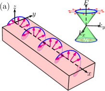
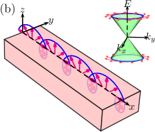
Figure 1: Illustration of spin helix of a chain of magnetic impurities. Two types of Dirac Hamiltonian, $\hat{H}^{a}_{0}$ and $\hat{H}^{b}_{0}$(see Model section), are considered, which lead to spin helix (magenta vectors) perpendicular(a) and parallel(b) to the chain direction, respectively. The insets show spin orientation of conduction electron in momentum space.

Model: We start from the Hamiltonian of the conduction electrons with only one Dirac cone

$$\hat{H}^{a}_{0}=\sum_{\mathbf{k}}\hat{c}^{\dagger}_{\mathbf{k}}(\hbar v_{F}\mathbf{k}\cdot\boldsymbol{\sigma}-E_{F}\mathbf{1})\hat{c}_{\mathbf{k}},$$ (1)

with Fermi energy $E_{F}$ and Pauli matrix $\boldsymbol{\sigma}$. Via a unitary transformation $\hat{a}_{\mathbf{k}s}=[\hat{c}_{\mathbf{k}\uparrow}+\text{sgn}(v_{F})se^{-i\theta_{\mathbf{k}}}\hat{c}_{\mathbf{k}\downarrow}]/\sqrt{2}$ with $\theta_{\mathbf{k}}$ the angle of vector $\mathbf{k}$ and $s=\pm 1$, it can be diagonalized as $\hat{H}^{a}_{0}=\sum_{s=\pm 1}(s\hbar|v_{F}|k-E_{f})\hat{a}^{\dagger}_{\mathbf{k}s}\hat{a}_{\mathbf{k}s}$. In practice, the recently discovered TI material, e.g., $\text{Bi}_{2}\text{Se}_{3}$ has surface state described by the Rashba type of Hamiltonian $\hat{H}^{b}_{0}=\sum_{\mathbf{k}}\hat{c}^{\dagger}_{\mathbf{k}}[\hbar v_{F}(\mathbf{k}\times\boldsymbol{\sigma})_{z}-E_{f}]\hat{c}_{\mathbf{k}}$Zhang2009 ; Xia2009 , which is related to $\hat{H}^{a}_{0}$ by a rotation of $\mathbf{k}$ around $z$ axis by $\pi/2$, hence we can focus on $\hat{H}^{a}_{0}$ in the following.

Suppose there are $N_{imp}$ impurity spins located at $\mathbf{r}_{n}$ denoted by $\mathbf{S}_{n}$, which interact with conduction electrons via the following spin-spin coupling

$$\hat{H}_{I}=\sum_{n=1}^{N_{imp}}\lambda_{z}\hat{s}^{z}(\mathbf{r}_{n})\hat{S}^{z}_{n}+\lambda_{\pm}[\hat{s}^{x}(\mathbf{r}_{n})\hat{S}^{x}_{n}+\hat{s}^{y}(\mathbf{r}_{n})\hat{S}^{y}_{n}],$$ (2)

where $\hat{s}^{x,y,z}(\mathbf{r})$ are the spin operators of the conduction electron at $\mathbf{r}$. The coupling constants are assumed to be isotropic in $xy$ plane $\lambda_{x}=\lambda_{y}\equiv\lambda_{\pm}$, but may differ from the $z$-component. The total Hamiltonian is simply the sum $\hat{H}=\hat{H}^{a,b}_{0}+\hat{H}_{I}$.

Before proceeding with the discussion of the effective interaction between impurity spins, we follow RKKYruderman1954 ; Kasuya1956 ; kei1957 to divide $\hat{H}_{I}$ into two parts: $\hat{H}_{I0}$ and $\hat{H}_{I1}$. $\hat{H}_{I0}$ consists of the diagonal term of $\hat{a}^{\dagger}_{\mathbf{k}s}\hat{a}_{\mathbf{k}s}$ and can be written as $\hat{H}_{I0}=\lambda_{\pm}\sum_{\mathbf{k}}(\mathbf{e}_{\mathbf{k}}\cdot\hat{\mathbf{s}}_{\mathbf{k}})\left(\mathbf{e}_{\mathbf{k}}\cdot\hat{\mathbf{S}}_{imp}\right)$, where $\mathbf{e}_{\mathbf{k}}=\mathbf{k}/k$, $\hat{\mathbf{s}}_{\mathbf{k}}=\hat{c}^{\dagger}_{\mathbf{k}}\boldsymbol{\sigma}\hat{c}_{\mathbf{k}}$, and $\hat{\mathbf{S}}_{imp}=\mathcal{V}^{-1}\sum_{n=1}^{N_{imp}}\hat{\mathbf{S}}_{n}$ is the density of impurity spin. And the remaining part is off-diagonal denoted by $\hat{H}_{I1}$. Notice that for the helical Hamiltonian, the electric current of the conduction electrons is proportional to their spins, for instance, $\hat{\mathbf{J}}=ev_{F}\sum_{\mathbf{k}}\hat{\mathbf{s}}_{\mathbf{k}}$ for $\hat{H}^{a}_{0}$, therefore $\hat{H}_{I0}$ actually implies a direct coupling between the electric current and the impurity spins, which provides a mechanism to control the impurity spins through the electric voltage for dilute impurity concentration.

RKKY interaction: For simplicity we focus on the case of two impurities at $\mathbf{r}_{1}$ and $\mathbf{r}_{2}$, respectively. The results given below via the symmetry analysis are also valid for many impurity case as long as we consider two-body interactions. The RKKY interaction can be obtained by integrating out the degree of freedom of conduction electrons, followed by an expansion to the second order of the coupling parameters $\lambda_{z,\pm}$ruderman1954 ; Kasuya1956 ; kei1957 . The effective interaction between impurity spins thus obtained contains only the even order terms for time reversal invariant system.

To the lowest order, the most general form of the interaction is $\hat{H}_{rkky}(\mathbf{r}_{12})=\sum_{\alpha_{1}\alpha_{2}}\Gamma_{\alpha_{1}\alpha_{2}}(\mathbf{r}_{12})\hat{S}^{\alpha_{1}}_{1}\hat{S}^{\alpha_{2}}_{2}$ with $\mathbf{r}_{12}\equiv\mathbf{r}_{1}-\mathbf{r}_{2}$. Without spin-orbit coupling as in the usual case, only terms with $\alpha_{1}=\alpha_{2}$ can exist due to a rotational symmetry in spin space. However, the situation is quite different for the helical metal, since $\hat{H}^{a}_{0}$ is invariant only under a joint rotation in both spin and orbital space, which allows more terms as soon become clear. Let us consider a global rotation around $z$ axis by $\varphi$ with the form $\hat{\mathbf{R}}_{\mathbf{e}_{z},\varphi}\equiv\exp[i\varphi\mathbf{e}_{z}\cdot\hat{\mathbf{s}}_{cond}]\times\exp[i\varphi\mathbf{e}_{z}\cdot(\hat{\mathbf{S}}_{1}+\hat{\mathbf{S}}_{2})]\times\exp[i\varphi\mathbf{e}_{z}\cdot\hat{\mathbf{L}}]$ with total spin of conduction electrons $\hat{\mathbf{s}}_{cond}=\int d\mathbf{r}\hat{c}^{\dagger}(\mathbf{r})\boldsymbol{\sigma}\hat{c}(\mathbf{r})/2$ and orbital angular momentum $\hat{\mathbf{L}}\equiv\int d\mathbf{r}\hat{c}^{\dagger}(\mathbf{r})(\mathbf{r}\times\mathbf{p})\hat{c}(\mathbf{r})$. Under this rotation, $\hat{H}^{a}_{0}$ is obviously invariant, but $\hat{H}_{I}(\mathbf{r}_{1},\mathbf{r}_{2})\rightarrow\hat{H}_{I}(\mathbf{r}^{\prime}_{1},\mathbf{r}^{\prime}_{2})$ with $\mathbf{r}^{\prime}\equiv e^{-i\varphi(xp_{y}-yp_{x})}\mathbf{r}e^{i\varphi(xp_{y}-yp_{x})}$, which breaks the rotational symmetry. However since the energy behaves like a scalar, one expects $\hat{H}_{rkky}(\mathbf{r}_{12})=\hat{H}_{rkky}(\mathbf{r}^{\prime}_{12})$, then what we are left with is to construct $\hat{\mathbf{R}}_{\mathbf{e},\varphi}$-invariants with vectors $\mathbf{e}_{12}(\equiv\mathbf{r}_{12}/r_{12})$, $\hat{\mathbf{S}}_{1}$ and $\hat{\mathbf{S}}_{2}$.

There are many such $\hat{\mathbf{R}}_{\mathbf{e}_{z},\varphi}$-invariants terms, most of which can be further eliminated by the following two symmetries. The first one is exchanging $\mathbf{r}_{1}$ and $\mathbf{r}_{2}$ which obviously leaves $\hat{H}$ invariant. Thus terms like $\mathbf{e}_{z}\cdot(\hat{\mathbf{S}}_{1}\times\hat{\mathbf{S}}_{2})$ are not allowed. The second one is a global rotation $\hat{\mathbf{R}}_{\mathbf{e}_{12},\pi}$ around axis $\mathbf{e}_{12}$ by $\pi$, which rules out invariants like $[\mathbf{e}_{12}\times(\mathbf{S}_{1}\times\mathbf{S}_{2})]_{z}$ that changes sign under rotation $\mathbf{R}_{\mathbf{e}_{12},\pi}$. Hence, we are left with the following two terms in addition to the conventional ones, $\mathbf{e}_{12}\cdot(\hat{\mathbf{S}}_{1}\times\hat{\mathbf{S}}_{2})$ and $(\mathbf{e}_{12}\cdot\hat{\mathbf{S}}_{1})(\mathbf{e}_{12}\cdot\hat{\mathbf{S}}_{2})$. One then constructs the effective Hamiltonian of impurity spins as

$$\hat{H}_{rkky}(\mathbf{r}_{12}) = \Gamma_{0}(r_{12})[\lambda^{2}_{\pm}(\hat{S}_{1}^{x}\hat{S}^{x}_{2}+\hat{S}_{1}^{y}\hat{S}^{y}_{2})+\lambda^{2}_{z}\hat{S}_{1}^{z}\hat{S}^{z}_{2}]$$ (3)

$$+\Gamma_{1}(r_{12})\lambda_{\pm}^{2}[(\mathbf{e}_{12}\cdot\hat{\mathbf{S}}_{1})(\mathbf{e}_{12}\cdot\hat{\mathbf{S}}_{2})]$$

$$+\Gamma_{DM}(r_{12})\lambda_{z}\lambda_{\pm}[\mathbf{e}_{12}\cdot(\hat{\mathbf{S}}_{1}\times\hat{\mathbf{S}}_{2})],$$

where the $\Gamma_{0}$-term is just the conventional RKKY terms.

Derivation of $\Gamma_{0,1,DM}$: The coefficients $\Gamma_{0,1,DM}$ in Eq. (3) can be computed following RKKY’s second order perturbationruderman1954 ; Kasuya1956 ; kei1957 . Let us consider the following generalized partition function which is partially traced over conduction electrons, $\mathcal{Z}=\text{Tr}_{\text{cond}}e^{-\beta(\hat{H}_{0}+\hat{H}_{I})}$. To the quadratic order of $\lambda_{z,\pm}$, we obtain

$$\frac{\mathcal{Z}}{\mathcal{Z}_{0}}\approx\exp\left\{\frac{\beta}{\mathcal{V}^{2}}\sum_{\mathbf{k}_{1}s_{1}}\sum_{\mathbf{k}_{2}s_{2}}\sum_{n,m}\frac{f_{\mathbf{k}_{1}s_{1}}(1-f_{\mathbf{k}_{2}s_{2}})}{\xi_{\mathbf{k}_{2}s_{2}}-\xi_{\mathbf{k}_{1}s_{1}}}[\sum_{a=x,y,z}\lambda_{a}F^{a}_{\mathbf{k}_{1}s_{1};\mathbf{k}_{2}s_{2}}\hat{S}^{a}_{n}][\sum_{b=x,y,z}\lambda_{b}F^{b}_{\mathbf{k}_{2}s_{2};\mathbf{k}_{1}s_{1}}\hat{S}^{b}_{m}]e^{i(\mathbf{r}_{m}-\mathbf{r}_{n})(\mathbf{k}_{1}-\mathbf{k}_{2})}\right\}$$ (4)

where $\mathcal{Z}_{0}$ is the partition function of conduction electrons, $f_{\mathbf{k}s}=[1+e^{\beta(s\hbar|v_{F}|k-E_{f})}]^{-1}$ is the Fermi distribution function, and the three $F$-functions take the forms $F^{x}_{\mathbf{k}_{1}s_{1};\mathbf{k}_{2}s_{2}}=\frac{1}{4}\text{sgn}(v_{F})(s_{1}e^{-i\theta_{\mathbf{k}_{1}}}+s_{2}e^{i\theta_{\mathbf{k}_{2}}})$, $F^{y}_{\mathbf{k}_{1}s_{1};\mathbf{k}_{2}s_{2}}=\frac{i}{4}\text{sgn}(v_{F})(s_{1}e^{-i\theta_{\mathbf{k}_{1}}}-s_{2}e^{i\theta_{\mathbf{k}_{2}}})$ and $F^{z}_{\mathbf{k}_{1}s_{1};\mathbf{k}_{2}s_{2}}=\frac{1}{4}(1-s_{1}s_{2}e^{-i(\theta_{\mathbf{k}_{1}}-\theta_{\mathbf{k}_{2}})})$, which depend only on $\theta_{\mathbf{k}_{1,2}}$, the angle of $\mathbf{k}_{1,2}$. By comparing with Eq. (3), one can extract the coefficients $\Gamma_{0,1,DM}$ from Eq. (4) straightforwardly. After integrating over $\theta_{\mathbf{k}_{1,2}}$, we have $\Gamma_{0}(r)=-2[A(r)-B(r)]$, $\Gamma_{1}(r)=-4B(r)$ and $\Gamma_{DM}(r)=-2C(r)$, where the functions $A$, $B$ and $C$ read in the zero temperature limit

$$A(r) = \frac{1}{8\hbar|v_{F}|r^{3}}\sum_{s_{1}s_{2}}\int x_{1}dx_{1}\int x_{2}dx_{2}\mathscr{J}_{0}(x_{1})\mathscr{J}_{0}(x_{2})$$

$$\hskip 28.45274pt\times\frac{\theta(x_{F}-x_{1})\theta(x_{2}-x_{F})}{s_{2}x_{2}-s_{1}x_{1}}$$

$$B(r) = \frac{1}{8\hbar|v_{F}|r^{3}}\sum_{s_{1}s_{2}}\int x_{1}dx_{1}\int x_{2}dx_{2}\mathscr{J}_{1}(x_{1})\mathscr{J}_{1}(x_{2})$$

$$\hskip 28.45274pt\times\frac{\theta(x_{F}-x_{1})\theta(x_{2}-x_{F})}{s_{2}x_{2}-s_{1}x_{1}}$$

$$C(r) = \frac{\text{sgn}(v_{F})}{8\hbar|v_{F}|r^{3}}\sum_{s_{1}s_{2}}\int x_{1}dx_{1}\int x_{2}dx_{2}$$ (5)

$$\hskip 5.69046pt[s_{1}\mathscr{J}_{1}(x_{1})\mathscr{J}_{0}(x_{2})-s_{2}\mathscr{J}_{0}(x_{1})\mathscr{J}_{1}(x_{2})]$$

$$\times\frac{\theta(x_{F}-x_{1})\theta(x_{2}-x_{F})}{s_{2}x_{2}-s_{1}x_{1}}$$

where $x\equiv kr$, $x_{F}=k_{F}r$, $\theta(x)$ is Heaviside step function, and $\mathscr{J}_{0,1}(x)$ are the first and second order Bessel functions, respectively. Note that $\Gamma_{0}(r)$ has already been obtained in Ref.liuQ2009 , which agrees with ours. It is the $\Gamma_{1}$ and $\Gamma_{DM}$ terms that have not been addressed before, and the physics discussed in this letter is essentially coming from them.

The numerical results of $\Gamma_{0,1,DM}(r)$ are plotted in Fig. 3 where a cutoff is set for $x$ and the Cauchy principle integration is understood when singularities are encountered in Eq. (Spin Helix of Magnetic Impurities in Two-dimensional Helical Metal). Despite of the oscillation of the conventional RKKY interaction with respect to $r$ for large $k_{F}$, it is interesting to note that the DM interaction is of the same order of the conventional ones, and depends on the sign of $v_{F}$ as seen from the expression of $C(r)$ in Eq. (Spin Helix of Magnetic Impurities in Two-dimensional Helical Metal).

Single-handed Spin Helix: To reveal the effect of DM interaction, we focus on a simple case of one-dimensional chain of impurities aligned with equal spacing $d$ along $x$-axis, and the corresponding Hamiltonian reads

$$\hat{H}_{imp} = \sum_{n}(-J_{z}\hat{S}^{z}_{n}\hat{S}^{z}_{n+1}-J_{y}\hat{S}^{y}_{n}\hat{S}^{y}_{n+1}+J_{x}\hat{S}^{x}_{n}\hat{S}^{x}_{n+1})$$ (6)

$$+J_{DM}(\hat{S}^{z}_{n}\hat{S}^{y}_{n+1}-\hat{S}^{y}_{n}\hat{S}^{z}_{n+1})$$

where $J_{z}=-\Gamma_{0}(d)\lambda^{2}_{z}$, $J_{y}=-\Gamma_{0}(d)\lambda^{2}_{\pm}$, $J_{x}=[\Gamma_{0}(d)+\Gamma_{1}(d)]\lambda^{2}_{\pm}$, and $J_{DM}=-\Gamma_{DM}(d)\lambda_{z}\lambda_{\pm}$. Here we consider the case for $k_{F}$ close to the Dirac point, where we can simply assume $J_{y,z}>J_{x}>0$ as can be read off in Fig. 2b for $r\approx 1$. The other situations including two dimensional arrays of magnetic impurities are left for future studies.

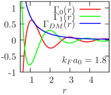
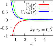
Figure 2: Plot of $\Gamma_{0,1,DM}$ as functions of the distance between impurities $r$, $k_{F}a_{0}=1.8$ (left) and $k_{F}a_{0}=0.5$ (right). The distance between impurities is in unit of lattice spacing $a_{0}$. The coefficient $8\hbar v_{F}a_{0}^{3}$ is taken as one for convenience.

In this case, the spins are lying in $yz$ plane in the classical limit. Therefore, we can introduce two variables $\hat{\theta}_{n}$ and $\hat{\rho}_{n}$ to describe the spin rotation in $yz$-plane and the amplitude fluctuation along $x$-axis, which satisfy the commutation relation $[\hat{\theta}_{n},\hat{\rho}_{m}]=i\delta_{m,n}$, and are related to $\hat{\mathbf{S}}_{n}$ through $\hat{S}^{x}_{n}=\hat{\rho}$, $\hat{S}^{y}_{n}+i\hat{S}^{z}_{n}=e^{i\hat{\theta}}[(S-\hat{\rho})(S+\hat{\rho}+1)]^{1/2}$ and $\hat{S}^{y}_{n}-i\hat{S}^{z}_{n}=[(S-\hat{\rho})(S+\hat{\rho}+1)]^{1/2}e^{-i\hat{\theta}}$. One may verify these equations satisfying the angular momentum algebra, and $\hat{\mathbf{S}}^{2}=S(S+1)$. In continuum limit the effective Hamiltonian for the dynamics of impurity spins can be written as

$$\hat{H}_{imp} = \int dx[-D_{1}\cos(d\partial_{x}\hat{\theta})+D_{2}\cos(2\hat{\theta})$$ (7)

$$+D_{3}\sin(d\partial_{x}\hat{\theta})+D_{0}\hat{\rho}^{2}]$$

with $[\hat{\theta}(x),\hat{\rho}(x^{\prime})]=i\delta(x-x^{\prime})$. The parameters are given by $D_{0}=J_{x}d$, $D_{1}=(J_{z}+J_{y})S(S+1)/(2d)$, $D_{2}=(J_{z}-J_{y})S(S+1)/(2d)$ and $D_{3}=J_{DM}S(S+1)/d$.

We first consider the isotropic case, i.e., $J_{z}=J_{y}$. The $\hat{\theta}(x)$ field has a helical background(see Fig. 1(a)), with helical angle $\eta$ satisfying $\tan(\eta d)=2J_{DM}/(J_{z}+J_{y})$. The sign of $\eta$ is the same as that of $J_{DM}$, and its amplitude is saturated to $\pi/2d$ as $J_{DM}$ is large enough as shown in the lower panel in Fig. 3. Replacing $\hat{\theta}(x)$ in Eq. (7) with $\eta x+\hat{\theta}(x)$, we have $\hat{H}_{imp}=\int dx[-\sqrt{D_{1}^{2}+D^{2}_{3}}\cos(d\partial_{x}\hat{\theta})+D_{0}\hat{\rho}^{2}]$ describing the quantum fluctuation upon the helical background. The low energy excitations can be obtained by expanding $\cos(d\partial_{x}\hat{\theta})$ to the second order of $d$, which leads to a linear spectrum in $k$ as $\omega_{k}=d(2D_{0})^{1/2}(D_{1}^{2}+D_{3}^{2})^{1/4}|k|$.

Next we consider the effect of spin anisotropy, i.e. $J_{z}\neq J_{y}$. Without loss of generality, we assume $J_{z}>J_{y}$(if $J_{z}<J_{y}$, one can shift $\hat{\theta}\rightarrow\hat{\theta}+\pi/2$ to get positive $D_{2}$). In this case the Hamiltonian becomes a sine-Gordon(SG) model $\hat{H}_{imp}\approx\int dx\frac{u}{2}[K^{-1}(\partial_{x}\hat{\theta})^{2}+K\hat{\rho}^{2}]+h\partial_{x}\hat{\theta}+D_{2}\cos(\sqrt{8\pi}\hat{\theta})$, which is written in the standard form by rescaling $\hat{\theta}$ and $\hat{\rho}$ in order to use the well known results in literature, e.g. in Refs.gogolin1998 ; yang2001 . The coefficients take the form $u=d\sqrt{J_{x}(J_{y}+J_{z})S(S+1)}$, $K=\pi^{-1}\sqrt{J_{x}/(J_{z}+J_{y})S(S+1)}$ and $h=\sqrt{2\pi}J_{DM}S(S+1)$. In case $K>1$, the cosine term is irrelevant, so that the system is massless and the spin helix takes place for any finite $h$. However in case $K<1$, the theory turns out to be massive, and a critical value of $|J_{DM}|$ exists, only above which the spin helix can occur in forms of massive soliton excitations of $\hat{\theta}$ fieldgogolin1998 ; yang2001 which connect different classical vacua of the SG model. In our case, since $0<J_{x}<J_{y,z}$, we are in the region of $K<1$. A schematic phase diagram for this case is given in the upper panel of Fig. 3, where the left helix, non-helical and right helix regions correspond to different topological sectors of sine-Gordon model with negative, zero, and positive topological charges, respectively.

Our analysis of DM interaction so far is focused on $\hat{H}^{a}_{0}$, where the spin helix is in $yz$ plane perpendicular to the impurity chain. For helical metal described by $\hat{H}^{b}_{0}$, the RKKY interaction can be obtained by rotating $\mathbf{e}_{12}$ around $z$-axis by $\pi/2$ in Eq. (3). As a consequence, the $\Gamma_{0}$-term is invariant, $\Gamma_{1}$-term becomes $\Gamma_{1}(r_{12})\lambda_{\pm}^{2}(\mathbf{e}_{12}\times\hat{\mathbf{S}}_{1})_{z}(\mathbf{e}_{12}\times\hat{\mathbf{S}}_{2})_{z}$ and $\Gamma_{DM}$-term becomes $\Gamma_{DM}(r_{12})\lambda_{\pm}\lambda_{z}[\mathbf{e}_{12}\times(\hat{\mathbf{S}}_{1}\times\hat{\mathbf{S}}_{2})]_{z}$. Notice that $(\mathbf{e}_{12}\times\hat{\mathbf{S}}_{1})_{z}(\mathbf{e}_{12}\times\hat{\mathbf{S}}_{2})_{z}=\hat{S}_{1}^{x}\hat{S}_{2}^{x}+\hat{S}_{1}^{y}\hat{S}_{2}^{y}-(\mathbf{e}_{12}\cdot\hat{\mathbf{S}}_{1})(\mathbf{e}_{12}\cdot\hat{\mathbf{S}}_{2})$, therefore $\Gamma_{1}$-term simply changes the coefficients of the first two terms of Eq. (3). Only the change of $\Gamma_{DM}$-term is essential, which makes the spin rotate in $xz$ plane instead of $yz$ plane as illustrated in Fig. 1b.

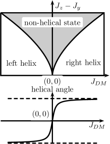
Figure 3: A schematic plot of phase diagram of $J_{z}-J_{y}$ vs. $J_{DM}$ in the upper panel for $K<1$, and helical angle as a function of $J_{DM}$ in lower panel. The left helix, non-helical state and right helix regions belong to different topological sectors of sine-Gordon model with negative, zero, and positive topological charges, respectively.

Summary: The surface state of TI is metallic with strong spin-orbit coupling, in which the magnetic impurities coupled with conductance electrons can be polarized by the electric voltage. There is also an effective interaction between impurity spins mediated by the conduction electrons, which includes a DM interaction with the same order of amplitude of the isotropic RKKY interactions. For 1D chain of impurities, this could lead to a single-handed spin helix, and the handedness is locked with the sign of Fermi velocity $v_{F}$ of the emergent Dirac particles.

References

(1)L. Fu, C. L. Kane, and E. J. Mele, Phys. Rev. Lett.98, 106803 (2007)
(2)J. E. Moore and L. Balents, Phys. Rev. B75, 121306 (2007)
(3)R. Roy, arXiv:cond-mat/0607531(2006)
(4)X.-L. Qi, T. L. Hughes, and S.-C. Zhang, Phys. Rev. B78, 195424 (2008)
(5)A. P. Schnyder, S. Ryu, A. Furusaki, and A. W. W. Ludwig, Phys. Rev. B78, 195125 (2008)
(6)C. Wu, B. A. Bernevig, and S.-C. Zhang, Phys. Rev. Lett.96, 106401 (2006)
(7)D. Hsieh, D. Qian, L. Wray, Y. Xia, Y. S. Hor, R. J. Cava, and M. Z. Hasan, Nature452, 970 (2008)
(8)H. Zhang, C.-X. Liu, X.-L. Qi, X. Dai, Z. Fang, and S.-C. Zhang, Nat Phys5, 438 (2009)
(9)Y. Xia, D. Qian, D. Hsieh, L. Wray, A. Pal, H. Lin, A. Bansil, D. Grauer, Y. S. Hor, R. J. Cava, and M. Z. Hasan, Nat Phys5, 398 (2009)