Unstable circular null geodesics of static spherically symmetric black holes,
Regge poles and quasinormal frequencies

Abstract

We consider a wide class of static spherically symmetric black holes of arbitrary dimension with a photon sphere (a hypersurface on which a massless particle can orbit the black hole on unstable circular null geodesics). This class includes various spacetimes of physical interest such as Schwarzschild, Schwarzschild-Tangherlini and Reissner-Nordström black holes, the canonical acoustic black hole or the Schwarzschild-de Sitter black hole. For this class of black holes, we provide general analytical expressions for the Regge poles of the $S$-matrix associated with a massless scalar field theory. This is achieved by using third-order WKB approximations to solve the associated radial wave equation. These results permit us to obtain analytically the nonlinear dispersion relation and the damping of the “surface waves” lying close to the photon sphere as well as, from Bohr-Sommerfeld–type resonance conditions, formulas beyond the leading-order terms for the complex frequencies corresponding to the weakly damped quasinormal modes.

I Introduction

Quasinormal modes (QNMs) of black holes (BHs) have been studied for nearly 40 years due to their importance in the context of gravitational wave astronomy. In the last decade, there has been moreover an increase of activity in BH QNM studies motivated by potential applications in analog models of gravity, quantum gravity, string theory and related topics (TeV-scale gravity, AdS/CFT correspondence, alternative theories of gravity, BH area quantization, phase transitions in BH systems,…). For excellent reviews on the status of QNMs prior to 1999 and on their relevance to gravitational wave astronomy, we refer to the articles by Kokkotas and Schmidt Kokkotas and Schmidt (1999) and by Nollert Nollert (1999). For a more recent review on BH QNMs, we refer to the article by Berti, Cardoso and Starinets Berti et al. (2009): it updates the two previously cited articles and it also presents the aspects of QNM physics linked to gauge-gravity duality; it includes, furthermore, an interesting historical introduction on the subject as well as a useful impressive bibliography on all the aspects of BH physics linked to QNMs.

Immediately after the publication of one of the first papers on QNMs by Press Press (1971) where he identified the gravitational ringing of the Schwarzschild BH as due to its “free oscillations”, Goebel suggested a physically intuitive interpretation of the associated QNMs Goebel (1972): they could be interpreted in terms of gravitational waves in spiral orbits close to the unstable circular photon/graviton orbit at $r=3M$ which decay by radiating away energy (here $M$ denotes the mass of the BH). This appealing interpretation has been developed by other authors for various field theories defined on BH backgrounds using the eikonal approximation, i.e., in a framework based on geodesics and bundle of geometrical rays (see Refs. Ferrari and Mashhoon (1984); Mashhoon (1985); Stewart (1989); Andersson and Onozawa (1996); Zerbini and Vanzo (2004); Cardoso et al. (2009); Dolan and Ottewill (2009); Hod (2009) as well as Ref. Sá Barreto and Zworski (1997) for a more mathematical approach). It has permitted them to obtain analytical approximations for the leading-order terms of the characteristic complex frequencies of various BH spectra from an interpretation in terms of massless particles “trapped” near unstable circular null geodesics (see, more particularly, Ref. Cardoso et al. (2009) where the relation with the Lyapunov exponent corresponding to geodesic motion is clearly emphasized).

A potentially much richer implementation of the Goebel interpretation of BH QNMs which is not limited to purely geometrical considerations but based on wave/field theory and which goes beyond the leading oder terms has also been formulated Décanini et al. (2003); Décanini and Folacci (2009, 2010) (see also Ref. Dolan and Ottewill (2009)). It uses complex angular momentum (CAM) techniques (or, in other words, the Regge pole machinery) which play a central role in scattering theory. Since, as noted by Chandrasekhar and coworkers Chandrasekhar (1983) (see also Ref. Ferrari (1992)), BH perturbation theory can be formulated as a resonant scattering problem, CAM techniques arise naturally in BH physics. For reviews of the CAM method, we refer to the monographs of Newton Newton (1982), Nussenzveig Nussenzveig (1992) and Collins Collins (1977) as well as to references therein for various applications in quantum mechanics, nuclear physics, high energy physics, electromagnetism and seismology.

Some years ago, the CAM method was used in gravitational wave physics by Chandrasekar and Ferrari Chandrasekhar and Ferrari (1992) to express the flow of energy due to nonradial oscillations of relativistic stars and by Andersson and Thylwe to describe scattering from the Schwarzschild BH Andersson and Thylwe (1994) as well as to interpret the Schwarzschild BH glory Andersson (1994). In this context, Andersson established, for the Schwarzschild BH of mass $M$, the existence of a family of “surface waves” (each one associated with a Regge pole of the $S$-matrix) orbiting close to the unstable photon orbit at $r=3M$ (see also Ref. Décanini et al. (2003) for a more rigorous approach). Recently, from these “surface waves”, we have been able to theoretically and numerically construct the spectrum of the weakly damped complex frequencies of the Schwarzschild BH QNMs Décanini et al. (2003); Décanini and Folacci (2010) and to interpret them as Breit-Wigner resonances. This has been achieved by obtaining analytically the nonlinear dispersion relation as well as the damping of the “surface waves” propagating close to the photon sphere. Let us also note two related papers concerning analytical or numerical determinations of the Regge poles of the Schwarzschild BH Glampedakis and Andersson (2003); Dolan and Ottewill (2009) and that, this last year, Regge poles have also been used to understand the resonant aspects of the BTZ BH Décanini and Folacci (2009) as well as to analyze some aspects of self-force calculations Casals et al. (2009).

In the present paper, we extend the analysis developed for the Schwarzschild BH to more general BHs and we establish, from Regge pole considerations, a precise connection between the existence of a photon sphere and the properties of the “surface waves” propagating close to it. More precisely, we consider a wide class of static spherically symmetric BHs of arbitrary dimension with a photon sphere, i.e., a hypersurface on which a massless particle can orbit the BH on unstable circular null geodesics. For more rigorous definitions of the photon sphere concept in static spherically symmetric spacetime, we refer to the article by Claudel, Virbhadra and Ellis Claudel et al. (2001). This class of BHs includes various spacetimes of physical interest such as Schwarzschild, Schwarzschild-Tangherlini and Reissner-Nordström BHs, the canonical acoustic BH or the Schwarzschild-de Sitter BH. For this class of BHs, we provide general analytical expressions beyond the leading-order terms for the Regge poles of the $S$-matrix associated with a massless scalar field theory. These results permit us to obtain analytically the nonlinear dispersion relation and the damping of the “surface waves” lying close to the photon sphere as well as, from Bohr-Sommerfeld–type resonance conditions, the complex frequencies corresponding to the weakly damped QNMs.

Our paper is organized as follows. In Sec. II, we display our general working assumptions and we justify them physically. We then explain how to construct the $S$-matrix permitting us to analyze the resonant aspects of a scalar field theory defined on an asymptotically flat static spherically symmetric BH of arbitrary dimension with a photon sphere and we finally define its Regge poles as well as its complex quasinormal frequencies. In Sec. III, we provide a general analytical expression for the Regge poles. This is achieved by using and extending the WKB approach developed in the context of the determination of the QNMs by Schutz and Will Schutz and Will (1985) and by Will and Iyer Iyer and Will (1987); Iyer (1987) (see also Ref. Bender and Orszag (1978) for general aspects of WKB theory and for particular aspects connected with eigenvalue problems). Our result permits us to describe the Regge trajectories of a general asymptotically flat static spherically symmetric BH of arbitrary dimension with a photon sphere and to obtain, from semiclassical formulas, analytical expressions for the QNM complex frequencies. Our WKB analysis permits us moreover to show that (i) the dispersion relation of the $n$th “surface wave” is nonlinear and depends on the index $n$ and that (ii) the damping of the $n$th “surface wave” is frequency dependent. In Sec. IV, we apply the general theory developed in Sec. III to particular BHs (Schwarzschild, Schwarzschild-Tangherlini, Reissner-Nordström and canonical acoustic BHs). In a brief conclusion, we consider some consequences of our work as well as possible extensions. In Appendix A, we establish the semiclassical connection between the Regge poles of a static spherically symmetric BH of arbitrary dimension with a photon sphere and the complex frequencies of its weakly damped QNMs. In Appendix B, we consider the particular case of the Schwarzschild-de Sitter BH. Indeed, even if such a gravitational background is not asymptotically flat, the formalism developed in Secs. II and III naturally applies to it.

In this paper, we shall use units with $\hbar=c=G=1$.

II Quasinormal frequencies and Regge poles of static spherically symmetric black holes: General theory

We consider a static spherically symmetric spacetime of arbitrary dimension $d\geq 4$ with metric

$$ds^{2}=-f(r)dt^{2}+\frac{dr^{2}}{f(r)}+r^{2}d\sigma_{d-2}^{2}.$$ (1)

Here $d\sigma_{d-2}^{2}$ denotes the line element on the unit sphere $S^{d-2}$. On $S^{d-2}$, we introduce the usual angular coordinates $\theta_{i}\in[0,\pi]$ with $i=1,\dots,d-3$ and $\varphi\in[0,2\pi]$. We have

$$d\sigma_{d-2}^{2}={d\theta_{1}}^{2}+\sum_{k=2}^{d-3}\left(\prod_{i=1}^{k-1}\sin^{2}\theta_{i}\right)d\theta_{k}^{2}+\left(\prod_{i=1}^{d-3}\sin^{2}\theta_{i}\right)d\varphi^{2}.$$ (2)

Of course, a metric such as (1) does not describe the most general static spherically symmetric spacetime but it will permit us to consider a wide class of BHs of physical interest.

In Eq. (1), we shall furthermore assume that $f(r)$ is a function of the usual radial coordinate $r$ with the following properties:

• (i) There exists an interval $I=]r_{h},+\infty[\subset\bf{R}$ with $r_{h}>0$ such as $f(r)>0$ for $r\in I$.

• (ii) $r_{h}$ is a simple root of $f(r)$, i.e.,

  $$f(r_{h})=0\qquad\text{and}\qquad f^{\prime}(r_{h})\neq 0,$$ (3)

  and $f(r)$ moreover satisfies

  $$\underset{r\to+\infty}{\lim}f(r)=1.$$ (4)

• (iii) There exists a value $r_{c}\in I$ for which

  $$f^{\prime}(r_{c})-\frac{2}{r_{c}}f(r_{c})=0$$ (5)

  and

  $$f^{\prime\prime}(r_{c})-\frac{2}{r_{c}^{2}}f(r_{c})<0.$$ (6)

We shall now briefly discuss assumptions (i)-(iii) previously introduced. Assumptions (i) and (ii) indicate that the spacetime considered is an asymptotically flat BH with an event horizon at $r_{h}$, its exterior corresponding to $r\in I$. Assumption (iii) implies the existence of a photon sphere which is the support of unstable circular null geodesics (see below for more details). It should be noted that, as a consequence of (i) and (ii), the tortoise coordinate $r_{\ast}=r_{\ast}(r)$ defined for $r\in I$ by the relation $dr_{\ast}/dr=1/f(r)$ and the condition $r_{\ast}(r_{c})=0$ provides a bijection $r_{\ast}=r_{\ast}(r)$ from $I$ to $]-\infty,+\infty[$.

Let us consider a free-falling massless particle orbiting the BH. Without loss of generality, we can consider that its motion lies on the equatorial hyperplane defined by $\theta_{i}=\pi/2$ for $i=1,\dots,d-3$. Because it moves along a null geodesic, we have [cf. Eqs. (1) and (2)]

$$-f(r)\left(\frac{dt}{d\alpha}\right)^{2}+\frac{1}{f(r)}\left(\frac{dr}{d\alpha}\right)^{2}+r^{2}\left(\frac{d\varphi}{d\alpha}\right)^{2}=0$$ (7)

where $\alpha$ is an affine parameter and, of course, there exist two integrals of motion respectively associated with the Killing vectors $\partial/\partial t$ and $\partial/\partial\varphi$ and given by

$$f(r)\left(\frac{dt}{d\alpha}\right)=E,$$ (8a)

$$r^{2}\left(\frac{d\varphi}{d\alpha}\right)=L.$$ (8b)

Here $E$ and $L$ denote respectively the energy and the angular momentum of the massless particle. Inserting Eqs. (8a) and (8b) into (7), we obtain

$$\left(\frac{dr}{d\alpha}\right)^{2}+V_{\mathrm{eff}}(r)=E^{2}$$ (9)

where

$$V_{\mathrm{eff}}(r)=\frac{L^{2}}{r^{2}}f(r).$$ (10)

From these last two equations and from assumption (iii), one can easily remark that the massless particle can orbit the BH on an unstable circular geodesic defined by $r=r_{c}$. Indeed, we have in particular

$$\left.\frac{d}{dr}V_{\mathrm{eff}}(r)\right|_{r=r_{c}}=0$$ (11a)

and

$$\left.\frac{d^{2}}{dr^{2}}V_{\mathrm{eff}}(r)\right|_{r=r_{c}}=\frac{L^{2}}{r_{c}^{2}}\left(f^{\prime\prime}(r_{c})-\frac{2}{r_{c}^{2}}f(r_{c})\right)<0.$$ (11b)

On this orbit, the massless particle takes the time

$$T=\frac{2\pi r_{c}}{\sqrt{f(r_{c})}}$$ (12)

to circle the BH. This result can be obtained by integrating Eq. (7).

The wave equation for a massless scalar field propagating on a general gravitational background is given by

$$\Box\Phi=g^{\mu\nu}\nabla_{\mu}\nabla_{\nu}\Phi=\frac{1}{\sqrt{-g}}\partial_{\mu}\left(\sqrt{-g}g^{\mu\nu}\partial_{\mu}\Phi\right)=0.$$ (13)

If the spacetime metric is given by (1), after separation of variables and the introduction of the radial partial wave functions $\Phi_{\ell}(r)$ with $\ell=0,1,2,\dots$, this wave equation reduces to the Regge-Wheeler equation

$$\frac{d^{2}\Phi_{\ell}}{dr_{*}^{2}}+\left[\omega^{2}-V_{\ell}(r)\right]\Phi_{\ell}=0.$$ (14)

[Here we have assumed a harmonic time dependence $\exp(-i\omega t)$ for the massless scalar field.] In Eq. (14), $V_{\ell}(r)$ is the Regge-Wheeler potential given by

$$V_{\ell}(r)=f(r)\left[\frac{\ell(\ell+d-3)}{r^{2}}\right. + \left.\frac{(d-2)(d-4)}{4r^{2}}f(r)\right.$$ (15)

$$+ \left.\left(\frac{d-2}{2r}\right)f^{\prime}(r)\right].$$

It should be noted that

• $\lim_{r\to r_{h}}V_{\ell}(r)=0$ and $\lim_{r\to+\infty}V_{\ell}(r)=0$ and therefore the solutions of the radial equation (14) have a behavior in $\exp(\pm i\omega r_{\ast})$ at the horizon and at infinity.

• For $\ell\gg 1$, $V_{\ell}(r)$ has a local maximum at $r=r_{c}$ because, in this limit, $V_{\ell}(r)$ and $V_{\mathrm{eff}}(r)$ are similar.

• For any finite value of $\ell$, the local maximum of $V_{\ell}(r)$ is close to $r=r_{c}$.

For a given angular momentum index $\ell$, the $S$-matrix element $S_{\ell}(\omega)$ is defined by seeking the solution of the Regge-Wheeler equation (14) which has a purely ingoing behavior at the event horizon $r=r_{h}$, i.e., which satisfies

$$\Phi_{\ell}(r)\underset{r_{*}\to-\infty}{\sim}T_{\ell}(\omega)e^{-i\omega r_{*}}$$ (16)

and which, at spatial infinity $r\to+\infty$, presents an asymptotic behavior of the form

$$\Phi_{\ell}(r)\underset{r_{*}\to+\infty}{\sim}e^{-i\omega r_{*}+i\left(\ell+\frac{d-3}{2}\right)\frac{\pi}{2}-i\frac{\pi}{4}}$$

$$\qquad\qquad\qquad-S_{\ell}(\omega)e^{+i\omega r_{*}-i\left(\ell+\frac{d-3}{2}\right)\frac{\pi}{2}+i\frac{\pi}{4}}.$$ (17)

We recall that the $S$-matrix permits us to analyze the resonant aspects of the considered BH as well as to construct the form factor describing the scattering of a monochromatic scalar wave (see Appendix A).

To describe semiclassically resonance phenomena, the dual structure of the $S$-matrix plays a crucial role. Indeed, the $S$-matrix is a function of both the frequency $\omega$ and the angular momentum index $\ell$. It can be analytically extended into the complex $\omega$-plane as well as into the complex $\lambda$-plane (CAM plane) with $\lambda=\ell+(d-3)/2$. From now on, we shall denote by $S_{\lambda-(d-3)/2}(\omega)$ this double analytical extension. For $\ell=\lambda-(d-3)/2\in\bf{N}$, the simple poles lying in the fourth quadrant of the complex $\omega$-plane [let us recall that they are also simple poles of $T_{\lambda-(d-3)/2}(\omega)$] are the complex frequencies of the QNMs. These modes are therefore solutions of the radial wave equation (14) which are purely outgoing at infinity and purely ingoing at the horizon. We shall denote by $\omega_{\ell n}=\omega^{(o)}_{\ell n}-i\Gamma_{\ell n}/2$ where $n\in{\bf N}^{\ast}$ the quasinormal frequencies. We recall that $\omega^{(o)}_{\ell n}>0$ and $\Gamma_{\ell n}>0$ represent respectively the frequency of the oscillation and the damping corresponding to the associated QNM. We assume that, in the immediate neighborhood of $\omega_{\ell n}$, $S_{\ell}(\omega)$ has the Breit-Wigner form, i.e.,

$$S_{\ell}(\omega)\propto\frac{\Gamma_{\ell n}/2}{\omega-\omega^{(o)}_{\ell n}+i\Gamma_{\ell n}/2}.$$ (18)

For a given value $\omega>0$ of the frequency, the simple poles lying in the first quadrant of the complex $\lambda$-plane are the so-called Regge poles. It should be noted that they are also poles of $T_{\lambda-(d-3)/2}(\omega)$ and therefore the associated modes (Regge modes) are purely outgoing at infinity and purely ingoing at the horizon. We shall denote the Regge poles by $\lambda_{n}(\omega)$, the index $n=1,2,\dots$ permitting us to distinguish each pole.

The structure of the $S$-matrix in the complex $\lambda$-plane allows us, by using integration contour deformations, Cauchy’s theorem and asymptotic analysis, to provide a semiclassical description of scattering (see Appendix A for more precisions). The curves traced out in the CAM plane by the Regge poles as a function of the frequency $\omega$ are the so-called Regge trajectories. They permit us to interpret Regge poles in terms of “surface waves” (see Appendix A): $\mathrm{Re}\,\lambda_{n}(\omega)$ provides the dispersion relation for the $n$th “surface wave” while $\mathrm{Im}\,\lambda_{n}(\omega)$ corresponds to its damping. Furthermore, from the Regge trajectories, we can semiclassically construct the resonance spectrum [see, in Appendix A, formulas (88), (90) and (91)]. The semiclassical formula (a Bohr-Sommerfeld–type quantization condition)

$$\mathrm{Re}\,\lambda_{n}\left(\omega^{(0)}_{\ell n}\right)=\ell+\frac{d-3}{2},\qquad\ell\in{\bf N}$$ (19)

provides the location of the excitation frequencies $\omega^{(0)}_{\ell n}$ of the resonances generated by $n$th “surface wave”, while a second semiclassical formula gives the widths of these resonances

$$\frac{\Gamma_{\ell n}}{2}=\left.\frac{\mathrm{Im}\,\lambda_{n}(\omega)[d/d\omega\,\mathrm{Re}\,\lambda_{n}(\omega)]}{[d/d\omega\,\mathrm{Re}\,\lambda_{n}(\omega)]^{2}+[d/d\omega\,\mathrm{Im}\,\lambda_{n}(\omega)]^{2}}\right|_{\omega=\omega^{(0)}_{\ell n}}.$$ (20)

It should be moreover noted that this formula reduces, in the frequency range where the condition $|d/d\omega\,\mathrm{Re}\,\lambda_{n}(\omega)|\gg|d/d\omega\,\mathrm{Im}\,\lambda_{n}(\omega)|$ is satisfied, to

$$\frac{\Gamma_{\ell n}}{2}=\left.\frac{\mathrm{Im}\,\lambda_{n}(\omega)}{d/d\omega\,\mathrm{Re}\,\lambda_{n}(\omega)}\right|_{\omega=\omega^{(0)}_{\ell n}}.$$ (21)

III WKB approximations for the Regge poles and semiclassical expressions of the complex quasinormal frequencies

In general, it is not possible to solve exactly the Regge-Wheeler equation (14) and therefore we can obtain only analytical approximations for the Regge poles and for the complex quasinormal frequencies. For example, the WKB approach developed in the general context of eigenvalue problems (for more details see Ref. Bender and Orszag (1978)) has been adapted for the determination of the Schwarzschild BH QNMs by Schutz and Will Schutz and Will (1985) and by Will and Iyer Iyer and Will (1987); Iyer (1987) and, in Ref. Décanini and Folacci (2010), for the determination of the Schwarzschild BH Regge poles. It can be extended to the more general case considered in this paper. By using third-order WKB approximations Iyer and Will (1987); Iyer (1987) for the Regge modes of Eq. (14), we find that the Regge poles $\lambda$ are the complex solutions of the equation

$$\omega^{2}=\left[V_{0}(\lambda)+{[-2V_{0}^{(2)}(\lambda)]}^{1/2}\,{\overline{\Lambda}}(\lambda,n)\right]$$

$$\qquad-i\,\alpha(n)\,{[-2V_{0}^{(2)}(\lambda)]}^{1/2}[1+{\overline{\Omega}}(\lambda,n)]$$ (22)

with $\omega>0$ and $n=1,2,3,\dots$. Here

$${\overline{\Lambda}}(\lambda,n)=\frac{1}{{[-2V_{0}^{(2)}(\lambda)]}^{1/2}}\left[\frac{1}{8}\frac{V_{0}^{(4)}(\lambda)}{V_{0}^{(2)}(\lambda)}\left(\frac{1}{4}+\alpha(n)^{2}\right)\right.$$

$$\qquad\left.-\frac{1}{288}\left(\frac{V_{0}^{(3)}(\lambda)}{V_{0}^{(2)}(\lambda)}\right)^{2}\left(7+60\,\alpha(n)^{2}\right)\right]$$ (23a)

and

$${\overline{\Omega}}(\lambda,n)=\frac{1}{[-2V_{0}^{(2)}(\lambda)]}\times$$

$$\qquad\left[\frac{5}{6912}\left(\frac{V_{0}^{(3)}(\lambda)}{V_{0}^{(2)}(\lambda)}\right)^{4}\left(77+188\,\alpha(n)^{2}\right)\right.$$

$$\qquad\left.-\frac{1}{384}\left(\frac{{[V_{0}^{(3)}(\lambda)]}^{2}V_{0}^{(4)}(\lambda)}{{[V_{0}^{(2)}(\lambda)]}^{3}}\right)\left(51+100\,\alpha(n)^{2}\right)\right.$$

$$\qquad\left.+\frac{1}{2304}\left(\frac{V_{0}^{(4)}(\lambda)}{V_{0}^{(2)}(\lambda)}\right)^{2}\left(67+68\,\alpha(n)^{2}\right)\right.$$

$$\qquad\left.+\frac{1}{288}\left(\frac{V_{0}^{(3)}(\lambda)V_{0}^{(5)}(\lambda)}{{[V_{0}^{(2)}(\lambda)]}^{2}}\right)\left(19+28\,\alpha(n)^{2}\right)\right.$$

$$\qquad\left.-\frac{1}{288}\left(\frac{V_{0}^{(6)}(\lambda)}{V_{0}^{(2)}(\lambda)}\right)\left(5+4\,\alpha(n)^{2}\right)\right].$$ (23b)

In Eqs. (III) and (23), we have introduced the notations

$$\alpha(n)=n-1/2$$ (24)

and, for $p\in{\bf N}$,

$$V_{0}^{(p)}(\lambda)=\left.\frac{d^{p}}{{dr_{*}}^{p}}V_{\lambda-(d-3)/2}(r_{*})\right|_{r_{*}={(r_{*})}_{0}}$$ (25)

with ${(r_{*})}_{0}$ which denotes the maximum of the function $V_{\lambda-(d-3)/2}(r_{*})$.

In order to solve Eq. (III), we need to express the asymptotic expansions for $|\lambda|\to+\infty$ of $V_{0}(\lambda)$ and $\left[-2V_{0}^{(2)}(\lambda)\right]^{1/2}$ and of the various ratios appearing in Eqs. (23) and (23). In order to simplify the results we have introduced the notations

$$f_{c}^{(p)}=f^{(p)}(r_{c})$$ (26)

and

$$\eta_{c}=\frac{1}{2}\sqrt{4f_{c}-2r_{c}^{2}f_{c}^{(2)}}.$$ (27)

It is worth noting that the $\eta_{c}$ parameter is directly linked to the second derivative (11b) of the effective potential (10) taken at $r=r_{c}$. As a consequence, it represents a kind of measure of the instability of the circular orbits lying on the photon sphere. In fact, it can be expressed in terms of the Lyapunov exponent $\Lambda_{c}$ corresponding to these orbits introduced in Ref. Cardoso et al. (2009) and which is the inverse of the instability time scale associated with them: we have

$$\eta_{c}=\frac{r_{c}}{\sqrt{f_{c}}}|\Lambda_{c}|.$$ (28)

We will say no more about this connection because, as already mentioned in Sec. I, we intend to go beyond purely geometrical considerations in our analysis of the resonant behavior of BHs.

After a tedious calculation, we obtain

$$V_{0}(\lambda)=\lambda^{2}\frac{f_{c}}{r_{c}^{2}}+\frac{f_{c}}{4r_{c}^{2}}\left[d(d-2)f_{c}-(d-3)^{2}\right]+\underset{|\lambda|\to+\infty}{\cal O}\left(\frac{1}{\lambda^{2}}\right)$$ (29a)

and

$$\left[-2V_{0}^{(2)}(\lambda)\right]^{1/2} = \frac{2\eta_{c}f_{c}}{r_{c}^{2}}\lambda-\frac{f_{c}}{8\eta_{c}^{3}r_{c}^{2}}\left[2f_{c}^{2}[(d-3)^{2}+(d-2)(d-4)f_{c}]\phantom{\left(f_{c}^{(2)}\right)^{2}}\right.$$ (29b)

$$\left.+r_{c}^{2}f_{c}f_{c}^{(2)}[(d-2)(d+8)f_{c}-2(d-3)^{2}]+d(d-2)r_{c}^{3}f_{c}^{2}f_{c}^{(3)}\phantom{\left(f_{c}^{(2)}\right)^{2}}\right.$$

$$\left.+r_{c}^{4}\left(f_{c}^{(2)}\right)^{2}[(1/2)(d-3)^{2}-(d^{2}-4)f_{c}]\right]\frac{1}{\lambda}+\underset{|\lambda|\to+\infty}{\cal O}\left(\frac{1}{\lambda^{3}}\right)$$

as well as

$$\frac{V_{0}^{(4)}(\lambda)}{V_{0}^{(2)}(\lambda)} = -\frac{f_{c}}{2\eta_{c}^{2}r_{c}^{2}}\left[16f_{c}^{2}-16r_{c}^{2}f_{c}f_{c}^{(2)}+4r_{c}^{3}f_{c}f_{c}^{(3)}\phantom{\left(f_{c}^{(2)}\right)^{2}}\right.$$ (30a)

$$\left.+r_{c}^{4}\left(4\left(f_{c}^{(2)}\right)^{2}+f_{c}f_{c}^{(4)}\right)\right]+\underset{|\lambda|\to+\infty}{\cal O}\left(\frac{1}{\lambda^{2}}\right),$$

$$\left(\frac{V_{0}^{(3)}(\lambda)}{V_{0}^{(2)}(\lambda)}\right)^{2}=\frac{r_{c}^{4}f_{c}^{2}\left(f_{c}^{(3)}\right)^{2}}{4\eta_{c}^{4}}+\underset{|\lambda|\to+\infty}{\cal O}\left(\frac{1}{\lambda^{2}}\right),$$ (30b)

$$\frac{{[V_{0}^{(3)}(\lambda)]}^{2}V_{0}^{(4)}(\lambda)}{{\left[V_{0}^{(2)}(\lambda)\right]}^{3}} = -\frac{r_{c}^{2}f_{c}^{3}\left(f_{c}^{(3)}\right)^{2}}{8\eta_{c}^{6}}\left[16f_{c}^{2}-16r_{c}^{2}f_{c}f_{c}^{(2)}+4r_{c}^{3}f_{c}f_{c}^{(3)}\phantom{\left(f_{c}^{(2)}\right)^{2}}\right.$$ (30c)

$$\left.+r_{c}^{4}\left(4\left(f_{c}^{(2)}\right)^{2}+f_{c}f_{c}^{(4)}\right)\right]+\underset{|\lambda|\to+\infty}{\cal O}\left(\frac{1}{\lambda^{2}}\right),$$

$$\frac{V_{0}^{(3)}(\lambda)V_{0}^{(5)}(\lambda)}{{\left[V_{0}^{(2)}(\lambda)\right]}^{2}} = \frac{r_{c}^{2}f_{c}^{3}f_{c}^{(3)}}{4\eta_{c}^{4}}\left[-10f_{c}f_{c}^{(3)}+10r_{c}f_{c}f_{c}^{(4)}\right.$$ (30d)

$$\left.+r_{c}^{2}\left(15f_{c}^{(2)}f_{c}^{(3)}+f_{c}f_{c}^{(5)}\right)\right]+\underset{|\lambda|\to+\infty}{\cal O}\left(\frac{1}{\lambda^{2}}\right),$$

$$\frac{V_{0}^{(6)}(\lambda)}{V_{0}^{(2)}(\lambda)}=-\frac{f_{c}^{2}}{2\eta_{c}^{2}r_{c}^{4}}\left[-272f_{c}^{3}+408r_{c}^{2}f_{c}^{2}f_{c}^{(2)}-88r_{c}^{3}f_{c}^{2}f_{c}^{(3)}\phantom{\left(f_{c}^{(2)}\right)^{2}}\right.$$

$$\qquad\left.+r_{c}^{4}f_{c}\left(38f_{c}f_{c}^{(4)}-204\left(f_{c}^{(2)}\right)^{2}\right)+r_{c}^{5}f_{c}\left(104f_{c}^{(2)}f_{c}^{(3)}+18f_{c}f_{c}^{(5)}\right)\phantom{\left(f_{c}^{(2)}\right)^{2}}\right.$$

$$\qquad\left.+r_{c}^{6}\left(34\left(f_{c}^{(2)}\right)^{3}+15f_{c}\left(f_{c}^{(3)}\right)^{2}+26f_{c}f_{c}^{(2)}f_{c}^{(4)}+f_{c}^{2}f_{c}^{(6)}\right)\right]+\underset{|\lambda|\to+\infty}{\cal O}\left(\frac{1}{\lambda^{2}}\right).$$ (30e)

We can now solve Eq. (III) by assuming $|\lambda|\gg 1$ as well as $\mathrm{Re}\,\lambda\gg\mathrm{Im}\,\lambda$. We obtain for the solutions a family $\lambda_{n}(\omega)$ with $n=1,2,3,\dots$ given by the approximation

$$\lambda_{n}(\omega)\approx\left[\frac{r_{c}^{2}}{f_{c}}\,\omega^{2}+a_{n}+2\eta_{c}^{2}\alpha(n)^{2}\epsilon_{n}(\omega)\right]^{1/2}+i\eta_{c}\alpha(n)\left[1+\epsilon_{n}(\omega)\right]$$ (31)

where

$$a_{n}=-~{}\frac{1}{1152\eta_{c}^{4}}\left\{288f_{c}^{2}\left[(d^{2}-2d-1)f_{c}-(d-3)^{2}\right]\phantom{\left(f_{c}^{(2)}\right)^{3}}\right.$$

$$\left.\quad+144r_{c}^{2}f_{c}f_{c}^{(2)}\left[2(d-3)^{2}-(2d^{2}-4d-3)f_{c}\right]\phantom{\left(f_{c}^{(2)}\right)^{3}}\right.$$

$$\left.\quad-72r_{c}^{3}f_{c}^{2}f_{c}^{(3)}-18r_{c}^{4}\left[4(d-3)^{2}\left(f_{c}^{(2)}\right)^{2}-4(d-3)(d+1)f_{c}\left(f_{c}^{(2)}\right)^{2}+f_{c}^{2}f_{c}^{(4)}\right]\right.$$

$$\left.\quad+36r_{c}^{5}f_{c}f_{c}^{(2)}f_{c}^{(3)}+\,r_{c}^{6}\left[36\left(f_{c}^{(2)}\right)^{3}-7f_{c}\left(f_{c}^{(3)}\right)^{2}+9f_{c}f_{c}^{(2)}f_{c}^{(4)}\right]\right\}$$

$$\quad+~{}\alpha(n)^{2}\frac{r_{c}^{3}f_{c}}{96\eta_{c}^{4}}\left\{24f_{c}f_{c}^{(3)}+6r_{c}f_{c}f_{c}^{(4)}-12r_{c}^{2}f_{c}^{(2)}f_{c}^{(3)}+r_{c}^{3}\left(5\left(f_{c}^{(3)}\right)^{2}-3f_{c}^{(2)}f_{c}^{(4)}\right)\right\}$$

and

$$\epsilon_{n}(\omega)=\frac{b_{n}}{(r_{c}^{2}/f_{c})\,\omega^{2}+a_{n}+\eta_{c}^{2}\alpha(n)^{2}}$$ (33)

with

$$b_{n}=\frac{1}{442368\eta_{c}^{10}}\left\{-55296(d-3)^{2}f_{c}^{5}(1+f_{c})+27648r_{c}^{2}f_{c}^{4}f_{c}^{(2)}\left[5(d-3)^{2}+2(d^{2}-12d+23)f_{c}\right]\right.$$

$$\left.\quad-9216(3d^{2}-6d-2)r_{c}^{3}f_{c}^{5}f_{c}^{(3)}+6912r_{c}^{4}f_{c}^{3}\left[-20(d-3)^{2}\left(f_{c}^{(2)}\right)^{2}+2(2d^{2}+36d-95)f_{c}\left(f_{c}^{(2)}\right)^{2}\right.\right.$$

$$\left.\left.\quad+9f_{c}^{2}f_{c}^{(4)}\right]+3456r_{c}^{5}f_{c}^{4}\left[6(2d^{2}-4d+1)f_{c}^{(2)}f_{c}^{(3)}+5f_{c}f_{c}^{(5)}\right]\right.$$

$$\left.\quad-192r_{c}^{6}f_{c}^{2}\left[-360(d-3)^{2}\left(f_{c}^{(2)}\right)^{3}+144(2d^{2}+6d-25)f_{c}\left(f_{c}^{(2)}\right)^{3}+423f_{c}^{2}f_{c}^{(2)}f_{c}^{(4)}-200f_{c}^{2}\left(f_{c}^{(3)}\right)^{2}\right.\right.$$

$$\left.\left.\quad-5f_{c}^{3}f_{c}^{(6)}\right]-96r_{c}^{7}f_{c}^{3}\left[36(6d^{2}-12d+17)\left(f_{c}^{(2)}\right)^{2}f_{c}^{(3)}-257f_{c}f_{c}^{(3)}f_{c}^{(4)}+270f_{c}f_{c}^{(2)}f_{c}^{(5)}\right]\right.$$

$$\left.\quad+12r_{c}^{8}f_{c}\left[-1440(d-3)^{2}\left(f_{c}^{(2)}\right)^{4}+288(7d^{2}+6d-55)f_{c}\left(f_{c}^{(2)}\right)^{4}+2376f_{c}^{2}\left(f_{c}^{(2)}\right)^{2}f_{c}^{(4)}\right.\right.$$

$$\left.\left.\qquad\qquad\quad+67f_{c}^{3}\left(f_{c}^{(4)}\right)^{2}+152f_{c}^{3}f_{c}^{(3)}f_{c}^{(5)}-2744f_{c}^{2}f_{c}^{(2)}\left(f_{c}^{(3)}\right)^{2}-120f_{c}^{3}f_{c}^{(2)}f_{c}^{(6)}\right]\right.$$

$$\left.\quad+48r_{c}^{9}f_{c}^{2}\left[12(6d^{2}-12d+59)\left(f_{c}^{(2)}\right)^{3}f_{c}^{(3)}+153f_{c}\left(f_{c}^{(3)}\right)^{3}-514f_{c}f_{c}^{(2)}f_{c}^{(3)}f_{c}^{(4)}+270f_{c}\left(f_{c}^{(2)}\right)^{2}f_{c}^{(5)}\right]\right.$$

$$\left.\quad+12r_{c}^{10}\left[144(d-3)^{2}\left(f_{c}^{(2)}\right)^{5}-288(d^{2}-7)f_{c}\left(f_{c}^{(2)}\right)^{5}-67f_{c}^{3}f_{c}^{(2)}\left(f_{c}^{(4)}\right)^{2}-152f_{c}^{3}f_{c}^{(2)}f_{c}^{(3)}f_{c}^{(5)}\right.\right.$$

$$\left.\left.\qquad\qquad+344f_{c}^{2}\left(f_{c}^{(2)}\right)^{2}\left(f_{c}^{(3)}\right)^{2}+60f_{c}^{3}\left(f_{c}^{(2)}\right)^{2}f_{c}^{(6)}+108f_{c}^{2}\left(f_{c}^{(2)}\right)^{3}f_{c}^{(4)}+153f_{c}^{3}\left(f_{c}^{(3)}\right)^{2}f_{c}^{(4)}\right]\right.$$

$$\left.\quad-24r_{c}^{11}f_{c}f_{c}^{(2)}\left[252\left(f_{c}^{(2)}\right)^{3}f_{c}^{(3)}+153f_{c}\left(f_{c}^{(3)}\right)^{3}-257f_{c}f_{c}^{(2)}f_{c}^{(3)}f_{c}^{(4)}+90f_{c}\left(f_{c}^{(2)}\right)^{2}f_{c}^{(5)}\right]\right.$$

$$\left.\quad+r_{c}^{12}\left[-864\left(f_{c}^{(2)}\right)^{6}+385f_{c}^{2}\left(f_{c}^{(3)}\right)^{4}-1512f_{c}\left(f_{c}^{(2)}\right)^{4}f_{c}^{(4)}-918f_{c}^{2}f_{c}^{(2)}\left(f_{c}^{(3)}\right)^{2}f_{c}^{(4)}\right.\right.$$

$$\left.\left.\qquad\quad+201f_{c}^{2}\left(f_{c}^{(2)}\right)^{2}\left(f_{c}^{(4)}\right)^{2}+456f_{c}^{2}\left(f_{c}^{(2)}\right)^{2}f_{c}^{(3)}f_{c}^{(5)}+1368f_{c}\left(f_{c}^{(2)}\right)^{3}\left(f_{c}^{(3)}\right)^{2}-120f_{c}^{2}\left(f_{c}^{(2)}\right)^{3}f_{c}^{(6)}\right]\right\}$$

$$\quad+\frac{\alpha(n)^{2}r_{c}^{3}f_{c}}{110592\eta_{c}^{10}}\left\{9216f_{c}^{4}f_{c}^{(3)}+13824r_{c}f_{c}^{4}f_{c}^{(4)}+3456r_{c}^{2}f_{c}^{3}\left[-2f_{c}^{(2)}f_{c}^{(3)}+f_{c}f_{c}^{(5)}\right]\phantom{\left(f_{c}^{(3)}\right)^{2}}\right.$$

$$\left.\quad+192r_{c}^{3}f_{c}^{3}\left[72\left(f_{c}^{(3)}\right)^{2}-99f_{c}^{(2)}f_{c}^{(4)}+f_{c}f_{c}^{(6)}\right]-288r_{c}^{4}f_{c}^{2}\left[12\left(f_{c}^{(2)}\right)^{2}f_{c}^{(3)}-29f_{c}f_{c}^{(3)}f_{c}^{(4)}+18f_{c}f_{c}^{(2)}f_{c}^{(5)}\right]\right.$$

$$\left.\quad+12r_{c}^{5}f_{c}^{2}\left[648\left(f_{c}^{(2)}\right)^{2}f_{c}^{(4)}+17f_{c}\left(f_{c}^{(4)}\right)^{2}+56f_{c}f_{c}^{(3)}f_{c}^{(5)}-1032f_{c}^{(2)}\left(f_{c}^{(3)}\right)^{2}-24f_{c}f_{c}^{(2)}f_{c}^{(6)}\right]\right.$$

$$\left.\quad+144r_{c}^{6}f_{c}\left[28\left(f_{c}^{(2)}\right)^{3}f_{c}^{(3)}+25f_{c}\left(f_{c}^{(3)}\right)^{3}-58f_{c}f_{c}^{(2)}f_{c}^{(3)}f_{c}^{(4)}+18f_{c}\left(f_{c}^{(2)}\right)^{2}f_{c}^{(5)}\right]\right.$$

$$\left.\quad+12r_{c}^{7}f_{c}\left[-36\left(f_{c}^{(2)}\right)^{3}f_{c}^{(4)}+75f_{c}\left(f_{c}^{(3)}\right)^{2}f_{c}^{(4)}-17f_{c}f_{c}^{(2)}\left(f_{c}^{(4)}\right)^{2}-56f_{c}f_{c}^{(2)}f_{c}^{(3)}f_{c}^{(5)}\right.\right.$$

$$\left.\left.\qquad\qquad\quad+168\left(f_{c}^{(2)}\right)^{2}\left(f_{c}^{(3)}\right)^{2}+12f_{c}\left(f_{c}^{(2)}\right)^{2}f_{c}^{(6)}\right]\right.$$

$$\left.\quad-72r_{c}^{8}f_{c}^{(2)}\left[12\left(f_{c}^{(2)}\right)^{3}f_{c}^{(3)}+25f_{c}\left(f_{c}^{(3)}\right)^{3}-29f_{c}f_{c}^{(2)}f_{c}^{(3)}f_{c}^{(4)}+6f_{c}\left(f_{c}^{(2)}\right)^{2}f_{c}^{(5)}\right]\right.$$

$$\left.\quad+r_{c}^{9}\left[235f_{c}\left(f_{c}^{(3)}\right)^{4}-216\left(f_{c}^{(2)}\right)^{4}f_{c}^{(4)}-450f_{c}f_{c}^{(2)}\left(f_{c}^{(3)}\right)^{2}f_{c}^{(4)}+51f_{c}\left(f_{c}^{(2)}\right)^{2}\left(f_{c}^{(4)}\right)^{2}\right.\right.$$

$$\left.\left.\qquad+168f_{c}\left(f_{c}^{(2)}\right)^{2}f_{c}^{(3)}f_{c}^{(5)}+360\left(f_{c}^{(2)}\right)^{3}\left(f_{c}^{(3)}\right)^{2}-24f_{c}\left(f_{c}^{(2)}\right)^{3}f_{c}^{(6)}\right]\right\}.$$ (34)

Equation (31) is the main result of our paper. As we shall see below (see also Appendix A), it also provides expressions for the dispersion relation and the damping of the “surface waves” lying on (close to) the photon sphere of the considered BH.

It is moreover possible to simplify (31) and to obtain a high frequency approximation for the Regge poles. We have

$$\lambda_{n}(\omega)=\left[\frac{r_{c}}{\sqrt{f_{c}}}~{}\omega+\frac{a_{n}}{(2r_{c}/\sqrt{f_{c}})}~{}\frac{1}{\omega}\right]+i\eta_{c}\alpha(n)\left[1+\frac{b_{n}}{(r_{c}^{2}/f_{c})}~{}\frac{1}{\omega^{2}}\right]+\underset{\omega\to+\infty}{\cal O}\left(\frac{1}{\omega^{3}}\right).$$ (35)

It is important to understand the difference between the approximation (31) and its much more elegant version (35). The approximation (35) is meaningful as a $1/\omega$ expansion with $\omega\to+\infty$. By contrast, the approximation (31) remains valid in a large range of frequencies thanks to WKB theory. Indeed, in order to establish Eq. (III) we have considered as a perturbation parameter of the WKB method the distance between the turning points of Eq. (14) [i.e., the roots of $Q_{\ell}(r^{\ast})=\omega^{2}-V_{\ell}(r^{\ast})$] and the location of the peak of $Q_{\ell}(r^{\ast})$ (see also Refs. Bender and Orszag (1978); Schutz and Will (1985); Iyer and Will (1987); Iyer (1987)) instead of $1/\omega$. Of course, in order to solve Eq. (III) and to obtain the expression (31), we have furthermore assumed that $|\lambda|\gg 1$ as well as $\mathrm{Re}\,\lambda\gg\mathrm{Im}\,\lambda$ and, as a consequence, we cannot expect from (31) a very high accuracy for very low frequencies (see also Refs. Dolan and Ottewill (2009) and Décanini and Folacci (2010) for related numerical studies in the case of the Schwarzschild BH).

It is furthermore interesting to provide an interpretation of the previous results in terms of “surface waves” as it is customary in the CAM approach. As we have noted in Appendix A, the resonant part of the form factor is a superposition of terms like $\exp[i(\lambda_{n}(\omega)\theta_{1}-\omega t)]$ (in this paragraph we take into account the harmonic time dependence $\exp[-i\omega t]$). By inserting the leading-order terms of Eq. (35) into these wavelike contributions, we can easily note that the contribution of the $n$th “surface wave” reduces to

$$\exp[-\eta_{c}\alpha(n)\theta_{1}]\,\exp\left[i\left(r_{c}/\sqrt{f_{c}}\,\omega\theta_{1}-\omega t\right)\right]$$ (36)

The second term describes the propagation of this “surface wave” near the photon sphere at $r=r_{c}$. Indeed, it circles the BH in time $T^{\prime}=2\pi(r_{c}/\sqrt{f_{c}})$ which is exactly the time (12) needed for a massless particle to orbit the BH on an unstable circular null geodesic. The first term corresponds to an exponential decay of this “surface wave” due to continual reradiation of energy. It is very interesting to rewrite Eq. (36) in the form

$$\exp[-k^{\prime\prime}_{n}(\omega){\cal L}]\exp[i(k^{\prime}_{n}(\omega){\cal L}-\omega t)]$$ (37)

with ${\cal L}=r_{c}\,\theta_{1}$ which denotes the arc length taken on the photon sphere. Now, $k^{\prime}_{n}(\omega)=\omega/\sqrt{f_{c}}$ represents the wavenumber of the $n$th “surface wave” or, in other terms, its dispersion relation, while $k^{\prime\prime}_{n}(\omega)=\eta_{c}\alpha(n)/r_{c}$ is its damping constant.

To the leading order, the dispersion relation is linear and independent of the index of the “surface wave” while the damping constant depends only on the index $n$. Of course, if we go beyond the leading-order terms, the dispersion relation reads [see Eq. (31)]

$$k^{\prime}_{n}(\omega)\approx\left[\frac{1}{f_{c}}\,\omega^{2}+\frac{a_{n}}{r_{c}^{2}}+2\left(\frac{\eta_{c}^{2}}{r_{c}^{2}}\right)\alpha(n)^{2}\epsilon_{n}(\omega)\right]^{1/2}$$ (38a)

which implies [see Eq. (35)]

$$k^{\prime}_{n}(\omega)=\left[\frac{1}{\sqrt{f_{c}}}~{}\omega+\frac{a_{n}}{(2r_{c}^{2}/\sqrt{f_{c}})}~{}\frac{1}{\omega}\right]+\underset{\omega\to+\infty}{\cal O}\left(\frac{1}{\omega^{3}}\right)$$ (38b)

and is clearly nonlinear as well as dependent on the index $n$. This result could have important consequences in strong gravitational lensing (see also Ref. Décanini and Folacci (2010) and the discussion in Appendix B.1 of the present paper). With such a potential application in mind, it is worth noting that, in Eqs. (37) and (38), $\omega$ denotes the frequency of the scalar photon observed by a static observer at infinity. If we consider the gravitational redshift of this photon and introduce its frequency ${\tilde{\omega}}=\omega/\sqrt{f_{c}}$ measured by a static observer lying on the photon sphere, the dispersion relation (38) reads

$$k^{\prime}_{n}({\tilde{\omega}})\approx\left[{\tilde{\omega}}^{2}+\frac{a_{n}}{r_{c}^{2}}+2\left(\frac{\eta_{c}^{2}}{r_{c}^{2}}\right)\alpha(n)^{2}\epsilon_{n}({\tilde{\omega}})\right]^{1/2}$$ (39a)

and we have

$$k^{\prime}_{n}({\tilde{\omega}})=\left[{\tilde{\omega}}+\frac{a_{n}}{2r_{c}^{2}}~{}\frac{1}{{\tilde{\omega}}}\right]+\underset{\omega\to+\infty}{\cal O}\left(\frac{1}{{\tilde{\omega}}^{3}}\right).$$ (39b)

When $a_{n}>0$, Eq. (39) provides a superluminal dispersion relation. Indeed, it leads to a group velocity $v_{g}({\tilde{\omega}})=d{\tilde{\omega}}/dk^{\prime}_{n}({\tilde{\omega}})>1$. The condition $a_{n}>0$ is satisfied $\forall n\in{\bf N}$ for spins 1 and 2 propagating on the Schwarzschild BH [see Eq. (13) of Ref. Décanini and Folacci (2010)]. It is also satisfied for the massless scalar field when $n\not=0$. As a consequence, it cannot be considered as an exotic physical condition. It even seems to be true in most cases encountered (see the examples considered in Sec. IV). At first sight, this result may seem a little bit puzzling. But it is important to note that superluminal dispersion relations for the “surface waves” lying on the photon sphere do not necessarily lead to a violation of the relativistic principle of causality. Indeed, for the transfer of information between a source and a receptor located outside a BH, various “channels” are involved. Of course, there are channels associated with diffraction by the BH photon sphere [for a source and a receptor at infinity, they correspond to the sum over the Regge poles in Eq. (A)] but there are also channels associated with geometrical rays [for a source and a receptor at infinity, they come from the background integral (A) over the contour $\Gamma$ of Fig. 1 after asymptotic evaluation]. In order to study causality, it would be necessary to carefully take into account interferences between all the monochromatic spectral components of the signal carrying the information for all the channels involved. We believe that such a study would not show a violation of causality. The situation encountered here is similar to that discussed by many authors working in electromagnetism of dispersive media (see, e.g., Ref. Brillouin (1960) and references therein). In such a context, it has been observed that a group velocity greater than the light velocity does not violate causality because it is not the velocity of information transmission or the energy velocity.

Finally, the WKB result (31) and the associated Regge trajectories permit us to derive, from the semiclassical formulas (19) and (21), useful analytical expressions for the QNM complex frequencies. Indeed, by inserting (31) into Eqs. (19) and (21), we obtain the large $\ell$ behaviors

$$\omega^{(o)}_{\ell n}=\frac{\sqrt{f_{c}}}{r_{c}}\left[\left(\ell+\frac{d-3}{2}\right)-\frac{a_{n}}{2\ell}+(d-3)\frac{a_{n}}{4\ell^{2}}+\underset{\ell\to+\infty}{\cal O}\left(\frac{1}{\ell^{3}}\right)\right],$$ (40a)

$$\frac{\Gamma_{\ell n}}{2}=\eta_{c}\frac{\sqrt{f_{c}}}{r_{c}}\alpha(n)\left[1+\frac{c_{n}}{2\ell^{2}}+\underset{\ell\to+\infty}{\cal O}\left(\frac{1}{\ell^{3}}\right)\right],$$ (40b)

with $\ell\in{\bf N}$ and $n=1,2,\dots$ Here

$$c_{n}=a_{n}+2b_{n}.$$ (41)

It should be noted that the leading-order terms of Eq. (40) have already been obtained in Refs. Zerbini and Vanzo (2004); Cardoso et al. (2009); Dolan and Ottewill (2009). The higher-order terms in $1/\ell$ and $1/\ell^{2}$ are new (see, however, Sec. 5.2 of Ref. Dolan and Ottewill (2009)). They are directly linked to the nonlinear behavior of both the dispersion relation and the damping of the “surface waves” lying on (close to) the photon sphere.

IV Applications

In this section we shall apply the previous formalism to various spacetimes of physical interest.

IV.1 Schwarzschild-Tangherlini black holes

For Schwarzschild-Tangherlini BHs Tangherlini (1963), the function $f(r)$ reads

$$f(r)=1-\left(\frac{r_{0}}{r}\right)^{d-3}$$ (42)

with

$$r_{0}^{d-3}=\frac{16\pi M}{(d-2){\cal A}_{d-2}}\quad\text{and}\quad{\cal A}_{d-2}=\frac{2\pi^{(d-1)/2}}{\Gamma[(d-1)/2]}.$$ (43)

Here $M$ is the mass of the BH, ${\cal A}_{d-2}$ the area of the unit sphere $S^{d-2}$ and the event horizon is located at $r_{h}=r_{0}$. The unstable circular null geodesics are located at

$$r_{c}=r_{0}\left(\frac{d-1}{2}\right)^{1/(d-3)}$$ (44a)

and the associated $$\eta_{c}$$ parameter is given by

$$\eta_{c}=\sqrt{d-3}.$$ (44b)

IV.1.1 d=4. The Schwarzschild black hole

For $d=4$, the Schwarzschild-Tangherlini solution is nothing but the ordinary Schwarzschild BH and we have

$$r_{c}=\frac{3}{2}r_{0}=3M,$$ (45a)

$$\eta_{c}=1,$$ (45b)

as well as

$$a_{n}=-\frac{29}{216}+\frac{5}{18}\alpha(n)^{2},$$ (46a)

$$b_{n}=\frac{1357}{15552}-\frac{305}{3888}\alpha(n)^{2},$$ (46b)

$$c_{n}=\frac{313}{7776}+\frac{235}{1944}\alpha(n)^{2},$$ (46c)

$$\epsilon_{n}(\omega)=\frac{b_{n}}{27M^{2}\omega^{2}+a_{n}+\alpha(n)^{2}}.$$ (46d)

The WKB approximation (31) for the Regge poles leads to

$$\lambda_{n}(\omega)\approx\left[27M^{2}\omega^{2}+a_{n}+2\alpha(n)^{2}\epsilon_{n}(\omega)\right]^{1/2}$$

$$\qquad+i\alpha(n)\left[1+\epsilon_{n}(\omega)\right]$$ (47)

and their high frequency behavior (35) provides

$$\lambda_{n}(\omega)=\left[3\sqrt{3}M\omega+\frac{\sqrt{3}a_{n}}{18M\omega}\right]$$

$$\qquad+i\alpha(n)\left[1+\frac{b_{n}}{27M^{2}\omega^{2}}\right]+\underset{\omega\to+\infty}{\cal O}\left(\frac{1}{\omega^{3}}\right).$$ (48)

Formulas (IV.1.1) and (IV.1.1) are in agreement with the results obtained in Ref. Décanini and Folacci (2010).

The resonance excitation frequencies and the damping of the QNMs given by the general formulas (40) reduce to

$$\omega_{\ell n}^{(0)}=\frac{1}{3\sqrt{3}M}\left[\left(\ell+\frac{1}{2}\right)-\frac{a_{n}}{2\ell}+\frac{a_{n}}{4\ell^{2}}+\underset{\ell\to+\infty}{\cal O}\left(\frac{1}{\ell^{3}}\right)\right],$$

(49a)

$$\frac{\Gamma_{\ell n}}{2}=\frac{\alpha(n)}{3\sqrt{3}M}\left[1+\frac{c_{n}}{2\ell^{2}}+\underset{\ell\to+\infty}{\cal O}\left(\frac{1}{\ell^{3}}\right)\right].$$ (49b)

Formulas (49) are in agreement with the results obtained in Ref. Iyer (1987) (see also Ref. Décanini and Folacci (2010)).

IV.1.2 The five-dimensional Schwarzschild-Tangherlini black hole

For $d=5$, we have

$$r_{c}=\sqrt{2}r_{0},$$ (50a)

$$\eta_{c}=\sqrt{2},$$ (50b)

as well as

$$a_{n}=-\frac{5}{16}+\frac{3}{4}\alpha(n)^{2},$$ (51a)

$$b_{n}=\frac{115}{512}-\frac{31}{128}\alpha(n)^{2},$$ (51b)

$$c_{n}=\frac{5}{48}+\frac{17}{64}\alpha(n)^{2},$$ (51c)

$$\epsilon_{n}(\omega)=\frac{b_{n}}{2r_{c}^{2}\,\omega^{2}+a_{n}+2\alpha(n)^{2}}.$$ (51d)

The WKB approximation (31) for the Regge poles leads to

$$\lambda_{n}(\omega)\approx\left[2r_{c}^{2}\omega^{2}+a_{n}+4\alpha(n)^{2}\epsilon_{n}(\omega)\right]^{1/2}$$

$$\qquad+i\alpha(n)[1+\epsilon_{n}(\omega)]$$ (52)

and their high frequency behavior (35) provides

$$\lambda_{n}(\omega)=\left[\sqrt{2}\,r_{c}\omega+\frac{a_{n}}{2\sqrt{2}\,r_{c}\omega}\right]$$

$$\qquad+i\sqrt{2}\,\alpha(n)\left[1+\frac{b_{n}}{2r_{c}^{2}\omega^{2}}\right]+\underset{\omega\to+\infty}{\cal O}\left(\frac{1}{\omega^{3}}\right).$$ (53)

The resonance excitation frequencies and the damping of the QNMs given by the general formulas (40) reduce to

$$\omega_{\ell n}^{(0)}=\frac{1}{\sqrt{2}\,r_{c}}\left[\left(\ell+1\right)-\frac{a_{n}}{2\ell}+\frac{a_{n}}{2\ell^{2}}+\underset{\ell\to+\infty}{\cal O}\left(\frac{1}{\ell^{3}}\right)\right],$$

(54a)

$$\frac{\Gamma_{\ell n}}{2}=\frac{\alpha(n)}{r_{c}}\left[1+\frac{c_{n}}{2\ell^{2}}+\underset{\ell\to+\infty}{\cal O}\left(\frac{1}{\ell^{3}}\right)\right].$$ (54b)

IV.1.3 The six-dimensional Schwarzschild-Tangherlini black hole

For $d=6$, we have

$$r_{c}=\left(\frac{5}{2}\right)^{1/3}r_{0},$$ (55a)

$$\eta_{c}=\sqrt{3},$$ (55b)

as well as

$$a_{n}=-\frac{31}{60}+\frac{7}{5}\alpha(n)^{2},$$ (56a)

$$b_{n}=\frac{1411}{3600}-\frac{91}{180}\alpha(n)^{2},$$ (56b)

$$c_{n}=\frac{481}{1800}+\frac{7}{18}\alpha(n)^{2},$$ (56c)

$$\epsilon_{n}(\omega)=\frac{b_{n}}{(5/3)r_{c}^{2}\,\omega^{2}+a_{n}+3\alpha(n)^{2}}.$$ (56d)

The WKB approximation (31) for the Regge poles leads to

$$\lambda_{n}(\omega)\approx\left[\frac{5}{3}r_{c}^{2}\omega^{2}+a_{n}+6\alpha(n)^{2}\epsilon_{n}(\omega)\right]^{1/2}$$

$$\qquad+i\sqrt{3}\alpha(n)\left[1+\epsilon_{n}(\omega)\right]$$ (57)

and their high frequency behavior (35) provides

$$\lambda_{n}(\omega)=\left[\left(\frac{5}{3}\right)^{1/2}r_{c}\omega+\frac{a_{n}}{2(5/3)^{1/2}r_{c}\omega}\right]$$

$$+i\sqrt{3}\,\alpha(n)\left[1+\frac{b_{n}}{(5/3)r_{c}^{2}\,\omega^{2}}\right]+\underset{\omega\to+\infty}{\cal O}\left(\frac{1}{\omega^{3}}\right).$$

The resonance excitation frequencies and the damping of the QNMs given by the general formulas (40) reduce to

$$\omega_{\ell n}^{(0)}=\left(\frac{3}{5}\right)^{1/2}\left(\frac{1}{r_{c}}\right)\left[\left(\ell+\frac{3}{2}\right)\phantom{\underset{\ell\to+\infty}{\cal O}\left(\frac{1}{\ell^{3}}\right)}\right.$$

$$\qquad\quad\left.-\frac{a_{n}}{2\ell}+3\frac{a_{n}}{4\ell^{2}}+\underset{\ell\to+\infty}{\cal O}\left(\frac{1}{\ell^{3}}\right)\right],$$ (59a)

$$\frac{\Gamma_{\ell n}}{2}=\sqrt{3}\left(\frac{3}{5}\right)^{1/2}\left(\frac{1}{r_{c}}\right)\alpha(n)$$

$$\qquad\quad\times\left[1+\frac{c_{n}}{2\ell^{2}}+\underset{\ell\to+\infty}{\cal O}\left(\frac{1}{\ell^{3}}\right)\right].$$ (59b)

IV.1.4 Leading-order terms for the Schwarzschild-Tangherlini black hole of arbitrary dimension

It should be noted that, in the $d$-dimensional case, we can easily derive the leading-order terms of the Regge poles and quasinormal complex frequencies. We have

$$\lambda_{n}(\omega)=\sqrt{\frac{d-1}{d-3}}\,r_{c}\omega+i\sqrt{d-3}\,\alpha(n)+\underset{\omega\to+\infty}{\cal O}\left(\frac{1}{\omega}\right)$$

and

$$\omega_{\ell n}^{(0)}=\sqrt{\frac{d-3}{d-1}}\left(\frac{1}{r_{c}}\right)\left(\ell+\frac{d-3}{2}\right)+\underset{\ell\to+\infty}{\cal O}\left(\frac{1}{\ell}\right),$$

(61a)

$$\frac{\Gamma_{\ell n}}{2}=\frac{d-3}{\sqrt{d-1}}\left(\frac{1}{r_{c}}\right)\alpha(n)+\underset{\ell\to+\infty}{\cal O}\left(\frac{1}{\ell}\right).$$ (61b)

Formulas (61) are in agreement with the results obtained in Refs. Konoplya (2003) and Zerbini and Vanzo (2004).

IV.2 The Reissner-Nordström black hole

For the $d$-dimensional Reissner-Nordström BH Tangherlini (1963), the function $f(r)$ reads

$$f(r)=1-\left(\frac{r_{0}}{r}\right)^{d-3}+\frac{\theta^{2}}{r^{2(d-3)}}$$ (62)

with (see Ref. Myers and Perry (1986) or Appendix A of Ref. Natário and Schiappa (2004))

$$r_{0}^{d-3}=\frac{16\pi M}{(d-2){\cal A}_{d-2}}\doteq 2\mu\quad\text{and}\quad\theta^{2}=\frac{8\pi q^{2}}{(d-2)(d-3)}.$$ (63)

Here $M$ is the mass of the BH and $q$ is its charge. We furthermore assume that $\mu^{2}>\theta^{2}$. It should be noted that here we consider electromagnetism in the Heaviside system of units. For this background there are two horizons, the so-called inner and outer horizons. They are respectively located at

$$r_{-}=\left(\mu-\sqrt{\mu^{2}-\theta^{2}}\right)^{1/(d-3)},$$ (64a)

$$r_{+}=\left(\mu+\sqrt{\mu^{2}-\theta^{2}}\right)^{1/(d-3)}.$$ (64b)

We are only interested in the outer horizon with radius at $r_{h}=r_{+}$ because we have $f(r)>0$ for $r\in]r_{h},+\infty[$ [see assumption (i) of Sec. II].

The unstable circular null geodesics are located at $r_{c}>r_{h}$ given by

$$r_{c}=\left(\frac{(d-1)\mu+\sqrt{[(d-1)\mu]^{2}-4(d-2)\theta^{2}}}{2}\right)^{1/(d-3)},$$ (65a)

and we have for the associated parameter $$\eta_{c}$$

$$\eta_{c}=\sqrt{(d-3)-\frac{(d-2)(d-3)\theta^{2}}{r_{c}^{2(d-3)}}}.$$ (65b)

For $\theta=0$ we recover the Schwarzschild-Tangherlini BH results. It should be noted that it is also possible to express $\eta_{c}$ in two other equivalent forms since, as a consequence of Eq. (5), the parameters $r_{c}$, $\mu$ and $\theta$ are linked by

$$\left(r_{c}^{d-3}\right)^{2}-(d-1)\mu r_{c}^{d-3}+(d-2)\theta^{2}=0.$$ (66)

IV.2.1 The four-dimensional Reissner-Nordström black hole

For $d=4$, we have

$$r_{c}=\frac{1}{2}(3M+\sqrt{9M^{2}-8Q^{2}}),$$ (67a)

$$\eta_{c}=\sqrt{1-\frac{2Q^{2}}{r_{c}^{2}}},$$ (67b)

as well as

$$a_{n}=\frac{\left(1-Q^{2}/r_{c}^{2}\right)^{2}}{216(1-2Q^{2}/r_{c}^{2})^{2}}\left[-29+\frac{86Q^{2}}{r_{c}^{2}}\right]+\frac{1-Q^{2}/r_{c}^{2}}{36(1-2Q^{2}/r_{c}^{2})^{2}}\left[10-\frac{62Q^{2}}{r_{c}^{2}}+\frac{124Q^{4}}{r_{c}^{4}}\right]\alpha(n)^{2},$$ (68a)

$$b_{n}=\frac{\left(1-Q^{2}/r_{c}^{2}\right)^{2}}{15552(1-2Q^{2}/r_{c}^{2})^{5}}\left[1357-\frac{12478Q^{2}}{r_{c}^{2}}+\frac{42333Q^{4}}{r_{c}^{4}}-\frac{64324Q^{6}}{r_{c}^{6}}+\frac{43588Q^{8}}{r_{c}^{8}}\right]$$

$$\quad+\frac{1-Q^{2}/r_{c}^{2}}{3888(1-2Q^{2}/r_{c}^{2})^{5}}\left[-305+\frac{3943Q^{2}}{r_{c}^{2}}-\frac{21335Q^{4}}{r_{c}^{4}}+\frac{56357Q^{6}}{r_{c}^{6}}-\frac{69544Q^{8}}{r_{c}^{8}}+\frac{34772Q^{10}}{r_{c}^{10}}\right]\alpha(n)^{2},$$ (68b)

$$c_{n}=\frac{\left(1-Q^{2}/r_{c}^{2}\right)^{2}}{7776(1-2Q^{2}/r_{c}^{2})^{5}}\left[313-\frac{3118Q^{2}}{r_{c}^{2}}+\frac{11229Q^{4}}{r_{c}^{4}}-\frac{18820Q^{6}}{r_{c}^{6}}+\frac{18820Q^{8}}{r_{c}^{8}}\right]$$

$$\quad+\frac{1-Q^{2}/r_{c}^{2}}{1944(1-2Q^{2}/r_{c}^{2})^{5}}\left[235-\frac{2645Q^{2}}{r_{c}^{2}}+\frac{11929Q^{4}}{r_{c}^{4}}-\frac{28315Q^{6}}{r_{c}^{6}}+\frac{37592Q^{8}}{r_{c}^{8}}-\frac{18796Q^{10}}{r_{c}^{10}}\right]\alpha(n)^{2},$$ (68c)

and

$$\epsilon_{n}(\omega)=\frac{b_{n}}{3r_{c}^{2}/(1-Q^{2}/r_{c}^{2})\,\omega^{2}+a_{n}+(1-2Q^{2}/r_{c}^{2})\alpha(n)^{2}}.$$ (68d)

Here we have noted $Q^{2}=4\pi q^{2}$. This permits us to compare our results with those for which electromagnetism is expressed in the Gaussian system of units. The WKB approximation (31) for the Regge poles leads to

$$\lambda_{n}(\omega)\approx\left[\frac{3r_{c}^{2}}{1-Q^{2}/r_{c}^{2}}\omega^{2}+a_{n}+2\left(1-\frac{2Q^{2}}{r_{c}^{2}}\right)\alpha(n)^{2}\epsilon_{n}(\omega)\right]^{1/2}+i\sqrt{1-\frac{2Q^{2}}{r_{c}^{2}}}\alpha(n)[1+\epsilon_{n}(\omega)]$$ (69)

and their high frequency behavior (35) provides

$$\lambda_{n}(\omega)=\left[\frac{\sqrt{3}\,r_{c}}{\sqrt{1-Q^{2}/r_{c}^{2}}}\omega+\frac{a_{n}}{2\sqrt{3}\,r_{c}/\sqrt{1-Q^{2}/r_{c}^{2}}\,\omega}\right]$$

$$\quad+i\sqrt{1-\frac{2Q^{2}}{r_{c}^{2}}}\alpha(n)\left[1+\frac{b_{n}}{3r_{c}^{2}/(1-Q^{2}/r_{c}^{2})\,\omega^{2}}\right]$$

$$\quad+\underset{\omega\to+\infty}{\cal O}\left(\frac{1}{\omega^{3}}\right).$$ (70)

The resonance excitation frequencies and the damping of the QNMs given by the general formulas (40) reduce to

$$\omega_{\ell n}^{(0)}=\sqrt{1-\frac{Q^{2}}{r_{c}^{2}}}\left(\frac{1}{\sqrt{3}\,r_{c}}\right)\left[\left(\ell+\frac{1}{2}\right)\phantom{\left(\frac{1}{\ell^{3}}\right)}\right.$$

$$\left.\qquad-\frac{a_{n}}{2\ell}+\frac{a_{n}}{4\ell^{2}}+\underset{\ell\to+\infty}{\cal O}\left(\frac{1}{\ell^{3}}\right)\right],$$ (71a)

$$\frac{\Gamma_{\ell n}}{2}=\sqrt{1-\frac{2Q^{2}}{r_{c}^{2}}}\sqrt{1-\frac{Q^{2}}{r_{c}^{2}}}\left(\frac{1}{\sqrt{3}\,r_{c}}\right)\,\alpha(n)$$

$$\qquad\times\left[1+\frac{c_{n}}{2\ell^{2}}+\underset{\ell\to+\infty}{\cal O}\left(\frac{1}{\ell^{3}}\right)\right].$$ (71b)

The leading-order terms of (71) are in agreement with formulas (37) and (38) of Ref. Ferrari and Mashhoon (1984). Furthermore, it should be noted that, for $Q=0$, all the results obtained for the Regge poles and the complex quasinormal frequencies of the four-dimensional Reissner-Nordström BH reduce to the Schwarzschild BH results of Sec. IV.A.1.

IV.2.2 Leading-order terms for the Reissner-Nordström black hole of arbitrary dimension

In the $d$-dimensional case, we can easily derive the leading-order terms of the Regge poles and quasinormal complex frequencies. We have

$$\lambda_{n}(\omega)=\sqrt{\frac{d-1}{d-3}}\frac{r_{c}\omega}{\sqrt{1-\frac{\theta^{2}}{r_{c}^{2(d-3)}}}}$$

$$\qquad+i\sqrt{d-3}\sqrt{1-\frac{(d-2)\theta^{2}}{r_{c}^{2(d-3)}}}\alpha(n)+\underset{\omega\to+\infty}{\cal O}\left(\frac{1}{\omega}\right)$$

and

$$\omega_{\ell n}^{(0)}=\sqrt{\frac{d-3}{d-1}}\sqrt{1-\frac{\theta^{2}}{r_{c}^{2(d-3)}}}\left(\frac{1}{r_{c}}\right)\left(\ell+\frac{d-3}{2}\right)$$

$$\qquad+\underset{\ell\to+\infty}{\cal O}\left(\frac{1}{\ell}\right),$$ (73a)

$$\frac{\Gamma_{\ell n}}{2}=\frac{d-3}{\sqrt{d-1}}\sqrt{1-\frac{\theta^{2}}{r_{c}^{2(d-3)}}}\sqrt{1-\frac{(d-2)\theta^{2}}{r_{c}^{2(d-3)}}}$$

$$\qquad\times\left(\frac{1}{r_{c}}\right)\alpha(n)+\underset{\ell\to+\infty}{\cal O}\left(\frac{1}{\ell}\right).$$ (73b)

It should be noted that for $\theta=0$, from (IV.2.2) and (73), we recover the Schwarzschild-Tangherlini BH results of Sec. IV.A.4.

IV.3 The canonical acoustic black hole

For the canonical acoustic BH (for more details see Sec. 8 of Ref. Visser (1998)), the function $f(r)$ reads

$$f(r)=1-\left(\frac{r_{0}}{r}\right)^{4}.$$ (74)

The sonic event horizon is located at $r_{h}=r_{0}$, the radius of the unstable circular null geodesics is given by

$$r_{c}=3^{1/4}r_{0}$$ (75a)

and we have for the corresponding $$\eta_{c}$$ parameter

$$\eta_{c}=2.$$ (75b)

Furthermore, we have

$$a_{n}=\frac{1}{108}+\frac{20}{9}\alpha(n)^{2},$$ (76a)

$$b_{n}=-\frac{85}{1944}-\frac{215}{243}\alpha(n)^{2},$$ (76b)

$$c_{n}=-\frac{19}{243}+\frac{110}{243}\alpha(n)^{2},$$ (76c)

$$\epsilon_{n}(\omega)=\frac{b_{n}}{(3/2)r_{c}^{2}\,\omega^{2}+a_{n}+4\alpha(n)^{2}}.$$ (76d)

The WKB approximation (31) for the Regge poles leads to

$$\lambda_{n}(\omega)\approx\left[\frac{3}{2}r_{c}^{2}\omega^{2}+a_{n}+8\alpha(n)^{2}\epsilon_{n}(\omega)\right]^{1/2}$$

$$\qquad+2i\alpha(n)\left[1+\epsilon_{n}(\omega)\right]$$ (77)

and their high frequency behavior (35) provides

$$\lambda_{n}(\omega)=\left[\frac{r_{c}}{\sqrt{2}}\omega+\frac{a_{n}}{\sqrt{2}\,r_{c}\omega}\right]$$

$$\qquad+2i\alpha(n)\left[1+\frac{b_{n}}{(3/2)r_{c}^{2}\omega^{2}}\right]+\underset{\omega\to+\infty}{\cal O}\left(\frac{1}{\omega^{3}}\right).$$

The resonance excitation frequencies and the damping of the QNMs given by the general formulas (40) reduce to

$$\omega_{\ell n}^{(0)}=\frac{\sqrt{2}}{r_{c}}\left[(\ell+1/2)-\frac{a_{n}}{2\ell}+\frac{a_{n}}{4\ell^{2}}+\underset{\ell\to+\infty}{\cal O}\left(\frac{1}{\ell^{3}}\right)\right],$$

(79a)

$$\frac{\Gamma_{\ell n}}{2}=\frac{2\sqrt{2}}{r_{c}}\alpha(n)\left[1+\frac{c_{n}}{2\ell^{2}}+\underset{\ell\to+\infty}{\cal O}\left(\frac{1}{\ell^{3}}\right)\right].$$ (79b)

The leading-order terms of (79) are in agreement with formula (53) of Ref. Berti et al. (2004). In Ref. Dolan and Ottewill (2009), Dolan and Ottewill have obtained for $n=0$ the expansions of $\omega_{\ell n}^{(0)}$ and $\Gamma_{\ell n}/2$ up to order $1/(\ell+1/2)^{4}$. Our results (79) are consistent with their Eq. (78).

V Conclusion

As noted by Chandrasekhar in the mid-1970s, BH perturbation theory can be formulated as a resonant scattering problem. As a consequence, all the techniques developed in the framework of scattering theory can be naturally introduced in the context of BH physics. One of the central concepts of scattering theory is the concept of a Regge pole which permits one to obtain semiclassical interpretations of resonance phenomena. We have recently used it in Refs. Décanini et al. (2003) and Décanini and Folacci (2010) in order to understand, from a new point of view, some aspects of the resonant Schwarzschild BH. Our results have permitted us to established more particularly, on a rigorous basis and in the wave/field theory context, the appealing and intuitive interpretation of Schwarzschild BH QNMs suggested by Goebel in 1972 Goebel (1972), i.e., that they could be interpreted in terms of gravitational waves in spiral orbits close to the unstable circular photon/graviton orbit at $r=3M$ which decay by radiating away energy.

In the present paper, we have greatly extended the approach initiated in Ref. Décanini and Folacci (2010). More precisely, we have provided general analytical formulas for the Regge poles of the $S$-matrix associated with a massless scalar field theory defined on a static spherically symmetric BH of arbitrary dimension with a photon sphere. This has been achieved by using third-order WKB approximations to solve the associated radial wave equation and by emphasizing more particularly the role of the photon sphere or, in other words, of the unstable circular null geodesics on which a massless particle can orbit the BH. But, it is important to note that our results are only a first step to understand, in a semiclassical framework, various aspects of static spherically symmetric BH physics such as wave scattering, gravitational lensing, Hawking radiation… Moreover, we think that it would now be very interesting to introduce the CAM method in a less symmetric situation, e.g., to study Kerr and Kerr-Newman BHs (see Ref. Glampedakis and Andersson (2003) for a first numerical step in this direction) and to analyze the splitting of their complex quasinormal frequencies or to understand, from a semiclassical point of view, the superradiance phenomenon. We leave such a study for the future.

Appendix A From Regge poles to complex quasinormal frequencies in arbitrary dimensions

In this appendix, we begin by extracting the resonant part of the form factor associated with the $S$-matrix defined in Sec. II. We then interpret it in terms of “surface waves”, each one associated with a Regge pole. This last result permits us to derive the semiclassical formulas (19)-(21) which are crucial to construct, in Sec. III, from the Regge trajectories, the spectrum of the complex frequencies corresponding to the weakly damped QNMs.

Let us consider the scattering of a monochromatic scalar plane wave of frequency $\omega$ by a $d$-dimensional static and spherically symmetric BH. Without loss of generality, the corresponding form factor can be written in the form

$$f(\omega,\theta_{1})=\frac{2^{\frac{d-4}{2}}}{2\sqrt{\pi}(i\omega)^{\frac{d-2}{2}}}\Gamma\left(\frac{d-3}{2}\right)$$

$$\quad\times\sum_{\ell=0}^{+\infty}(2\ell+d-3)\left[S_{\ell}(\omega)-1\right]C_{\ell}^{\frac{d-3}{2}}(\cos\theta_{1})$$

where $\ell$ is the ordinary angular momentum index, $C_{\ell}^{\frac{d-3}{2}}(z)$ are the Gegenbauer polynomials (see, for example, Ref. Abramowitz and Stegun (1965)) and $S_{\ell}(\omega)$ are the diagonal elements of the $S$-matrix defined by Eq. (II). By means of a Sommerfeld-Watson transformation Watson (1918); Sommerfeld (1949) (see for example Ref. Newton (1982) for a more recent presentation), we can extract in two steps the resonant part of the form factor (A). We first replace the discrete sum over the ordinary angular momentum $\ell$ by a contour integral in the complex $\lambda$-plane. We obtain

$$f(\omega,\theta_{1})=i\,\frac{2^{\frac{d-4}{2}}}{2\sqrt{\pi}(i\omega)^{\frac{d-2}{2}}}\Gamma\left(\frac{d-3}{2}\right)$$

$$\quad\times\int_{\cal C}\,\frac{\lambda\left[S_{\lambda-\frac{d-3}{2}}(\omega)-1\right]}{\sin[\pi(\lambda-(d-3)/2)]}C_{\lambda-\frac{d-3}{2}}^{\frac{d-3}{2}}(-\cos\theta_{1})~{}d\lambda.$$

Here $\mathcal{C}$ is the integration contour in the complex $\lambda$-plane displayed in Fig. 1. Furthermore, $S_{\lambda-(d-3)/2}(\omega)$ is now the analytic extension of $S_{\ell}(\omega)$ into the complex $\lambda$-plane (CAM plane) which is regular in the vicinity of the positive real $\lambda$ axis, and $C_{\lambda-\frac{d-3}{2}}^{\frac{d-3}{2}}(z)$ is the analytical extension of the Gegenbauer polynomials which is defined by Abramowitz and Stegun (1965)

$$C_{\lambda-\frac{d-3}{2}}^{\frac{d-3}{2}}(z)=\frac{\Gamma\left(\lambda+\frac{d-3}{2}\right)}{{\Gamma(d-3)\Gamma\left(\lambda-\frac{d-5}{2}\right)}}$$

$$\times F\left(-\lambda+\frac{d-3}{2},\lambda+\frac{d-3}{2};\frac{d-2}{2};\frac{1-z}{2}\right).$$ (82)

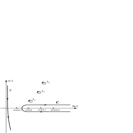
Figure 1: The Watson integration contour.

We can then deform the path of integration in Eq. (A) taking into account the possible singularities (see Fig. 1), i.e., the poles of the $S$-matrix lying in the first quadrant of the CAM plane, or in other words, the Regge poles $\lambda_{n}(\omega)$ with $n=1,2,\dots$ By Cauchy’s theorem we can then extract from Eq. (A) a residue series over Regge poles which permits us to obtain the resonant contribution in the form

$$f_{\mathrm{P}}(\omega,\theta_{1})=-2\pi\,\frac{2^{\frac{d-4}{2}}}{2\sqrt{\pi}(i\omega)^{\frac{d-2}{2}}}\Gamma\left(\frac{d-3}{2}\right)$$

$$\times\sum_{n=1}^{+\infty}\frac{\lambda_{n}(\omega)r_{n}(\omega)}{\sin\left[\pi(\lambda_{n}(\omega)-(d-3)/2)\right]}C_{\lambda_{n}(\omega)-\frac{d-3}{2}}^{\frac{d-3}{2}}(-\cos\theta_{1}).$$

Here we have defined

$$r_{n}(\omega)=\mathrm{residue}\left[S_{\lambda-(d-3)/2}(\omega)\right]_{\lambda=\lambda_{n}(\omega)}.$$ (84)

It should be noted that $f(\omega,\theta_{1})$ differs from $f_{\mathrm{P}}(\omega,\theta_{1})$ by a background integral over the contour $\Gamma$ (see Fig. 1) which does not play any role in resonance phenomena.

By using the asymptotic expansion (see Ref. Abramowitz and Stegun (1965))

$$C_{\lambda-\frac{d-3}{2}}^{\frac{d-3}{2}}(-\cos\theta_{1})\sim\frac{\Gamma\left(\frac{d-2}{2}\right)\Gamma\left(\lambda+\frac{d-3}{2}\right)}{\Gamma\left(d-3\right)\Gamma\left(\lambda+\frac{1}{2}\right)}$$

$$\quad\times\frac{e^{i\lambda(\pi-\theta_{1})-i(d-3)\pi/4}+e^{-i\lambda(\pi-\theta_{1})+i(d-3)\pi/4}}{2[{\pi(\lambda-(d-3)/2)}]^{1/2}[({\sin\theta_{1}})/2]^{(d-3)/2}}$$

as $|\lambda|\to\infty$, which is valid for $|\lambda|\sin\theta_{1}>1$, as well as the relation

$$\frac{1}{\sin\pi z}=-2i\sum_{m=0}^{+\infty}e^{i\pi(2m+1)z}$$ (86)

which is true if $\mathrm{Im}\ z>0$, we can write

$$f_{\mathrm{P}}(\omega,\theta_{1})=\frac{2i\pi}{(2i\omega)^{\frac{d-2}{2}}}\sum_{n=1}^{+\infty}\frac{\Gamma\left[\lambda_{n}(\omega)+(d-3)/2\right]}{\Gamma\left[\lambda_{n}(\omega)+1/2\right]}\frac{\lambda_{n}(\omega)r_{n}(\omega)e^{-i\pi(d-3)/2}}{[{\pi(\lambda_{n}(\omega)-(d-3)/2)}]^{1/2}[({\sin\theta_{1}})/2]^{(d-3)/2}}$$

$$\quad\times\sum_{m=0}^{+\infty}\left[e^{i\lambda_{n}(\omega)(2\pi-\theta_{1}+2m\pi)-i(d-3)m\pi-i(d-3)\pi/4}+e^{i\lambda_{n}(\omega)(\theta_{1}+2m\pi)-i(d-3)m\pi+i(d-3)\pi/4}\right].$$ (87)

In Eq. (A), exponential terms correspond to “surface wave”/diffractive contributions. Keeping in mind the time dependence $\exp(-i\omega t)$ and recalling that a given Regge pole $\lambda_{n}(\omega)$ lies in the first quadrant of the CAM plane, $\exp[i\lambda_{n}(\omega)(\theta_{1})]$ (resp. $\exp[i\lambda_{n}(\omega)(2\pi-\theta_{1})]$) corresponds to the so-called $n$th “surface wave” propagating counterclockwise (resp. clockwise) around the BH and $\mathrm{Re}\ \lambda_{n}(\omega)$ represents its azimuthal propagation constant while $\mathrm{Im}\ \lambda_{n}(\omega)$ is its damping constant. The corresponding exponential decay $\exp[-\mathrm{Im}\ \lambda_{n}(\omega)\theta_{1}]$ (resp. $\exp[-\mathrm{Im}\ \lambda_{n}(\omega)(2\pi-\theta_{1})]$) is due to continual reradiation of energy. Moreover, in Eq. (A), the sum over $m$ takes into account the multiple circumnavigations of the “surface waves” around the BH as well as the associated radiation damping. Finally, it should be noted that, in Eq. (A), the presence of the factor $\exp[-i(d-3)m\pi]$ accounts for the phase advance due to caustics.

The resonant behavior of the BH can now be understood in terms of “surface waves”. Let us consider the $n$th “surface wave”, i.e., the “surface wave” described by the Regge pole $\lambda_{n}(\omega)$. When the quantity $\mathrm{Re}\ \lambda_{n}(\omega)-(d-3)/2$ coincides with an integer, a resonance occurs: it is produced by a constructive interference between the different components of the surface wave, each component corresponding to a different number of circumnavigations of the BH [see Eq. (A)]. the resonance excitation frequencies $\omega^{(0)}_{\ell n}$ appearing in the Breit-Wigner formula (18) and generated by the $n$th “surface wave” are therefore obtained from the Bohr-Sommerfeld–type quantization condition

$$\mathrm{Re}\,\lambda_{n}\left(\omega^{(0)}_{\ell n}\right)=\ell+\frac{d-3}{2},\qquad\ell\in{\bf N}.$$ (88)

Now, by assuming that $\omega$ is in the neighborhood of $\omega^{(0)}_{\ell n}$, we can expand $\lambda_{n}(\omega)$ in a Taylor series about $\omega^{(0)}_{\ell n}$ and write

$$\lambda_{n}(\omega)\approx\ell+\frac{d-3}{2}+\left.\frac{d\,\mathrm{Re}\,\lambda_{n}(\omega)}{d\omega}\right|_{\omega=\omega^{(0)}_{\ell n}}\left(\omega-\omega^{(0)}_{\ell n}\right)$$

$$\quad+i\,\mathrm{Im}\,\lambda_{n}\left(\omega^{(0)}_{\ell n}\right)+i\left.\frac{d\,\mathrm{Im}\,\lambda_{n}(\omega)}{d\omega}\right|_{\omega=\omega^{(0)}_{\ell n}}\left(\omega-\omega^{(0)}_{\ell n}\right)$$

$$\quad+\dots$$ (89)

Then, by replacing (A) in the term ${\sin\left[\pi(\lambda_{n}(\omega)-(d-3)/2)\right]}$ of (A), we can see that $f_{\mathrm{P}}(\omega,\theta_{1})$ presents a resonant behavior given by the Breit-Wigner formula (18) with

$$\frac{\Gamma_{\ell n}}{2}=\left.\frac{\mathrm{Im}\,\lambda_{n}(\omega)[d/d\omega\,\mathrm{Re}\,\lambda_{n}(\omega)]}{[d/d\omega\,\mathrm{Re}\,\lambda_{n}(\omega)]^{2}+[d/d\omega\,\mathrm{Im}\,\lambda_{n}(\omega)]^{2}}\right|_{\omega=\omega^{(0)}_{\ell n}}.$$ (90)

Furthermore, it should be noted that in the frequency range where the condition $|d/d\omega\,\mathrm{Re}\,\lambda_{n}(\omega)|\gg|d/d\omega\,\mathrm{Im}\,\lambda_{n}(\omega)|$ is satisfied, (90) reduces to

$$\frac{\Gamma_{\ell n}}{2}=\left.\frac{\mathrm{Im}\,\lambda_{n}(\omega)}{d/d\omega\,\mathrm{Re}\,\lambda_{n}(\omega)}\right|_{\omega=\omega^{(0)}_{\ell n}}.$$ (91)

From the Regge trajectories, i.e., the curves traced out in the CAM plane by the functions $\lambda_{n}(\omega)$ for $\omega\in[0,+\infty[$, formulas (88) and (90) or (91) permit us to construct semiclassically the resonance spectrum of the BH or, in other words, the spectrum of the quasinormal complex frequencies. Equation (88) provides the location of the excitation frequencies $\omega^{(0)}_{\ell n}$ of these complex resonances while Eq. (90) provides the corresponding widths. Of course, the reasoning leading to (88) and (90) from (A) is based on many assumptions that are not necessarily satisfied in practice. But, in general, it permits one to describe rather correctly quasinormal complex frequencies lying near the real $\omega$-axis.

Appendix B Regge poles and QNMs of the Schwarzschild-de Sitter black hole

For the $d$-dimensional Schwarzschild-de Sitter BH Tangherlini (1963), the function $f(r)$ reads

$$f(r)=1-\left(\frac{r_{0}}{r}\right)^{d-3}-\frac{r^{2}}{L^{2}}.$$ (92)

Here, $r_{0}$ is a parameter associated with the mass $M$ of the BH by Eq. (43) and $L$ is a characteristic length linked to the cosmological constant $\Lambda$ by the relation

$$\Lambda=\frac{(d-1)(d-2)}{2L^{2}}.$$ (93)

If

$$0<\left(\frac{d-1}{2}\right)^{2/(d-1)}\left[\left(\frac{d-1}{d-3}\right)\frac{r_{0}^{2}}{L^{2}}\right]^{(d-3)/(d-1)}<1$$

the equation $f(r)=0$ has only two real roots $r_{h}$ and $r_{\mathrm{Co}}$ with $0<r_{h}<r_{\mathrm{Co}}$ (see, for example, Appendix A of Ref. Natário and Schiappa (2004)). They correspond to the radii of the BH horizon and of the cosmological horizon. For $r\in]r_{h},r_{\mathrm{Co}}[$, we have $f(r)>0$. In that case, there also exists a photon sphere located at

$$r_{c}=r_{0}\left(\frac{d-1}{2}\right)^{1/(d-3)}$$ (95a)

with $$r_{c}\in]r_{h},r_{\mathrm{Co}}[ \eta_{c}$$ and the associated parameter is given by

$$\eta_{c}=\sqrt{d-3}.$$ (95b)

$r_{c}$ and $\eta_{c}$ are both independent of the cosmological constant and are those already obtained for the ordinary Schwarzschild-Tangherlini BH [compare with Eqs. (44a) and (44b)].

Here, it is important to note that, at first sight, the formalism we have previously developed does not apply to this gravitational background which is not asymptotically flat and for which the function $f(r)$ is positive only in the finite interval $]r_{h},r_{\mathrm{Co}}[$. In particular, the proof of the semiclassical formulas (19)-(21) given in Appendix A is not valid because it is based on the notions of $S$-matrix and form factor which, here, cannot be used. But we can easily circumvent these difficulties:

• Indeed, for $f(r)$ given by (92) the potential $V_{\ell}(r)$ obtained from (15) satisfies the boundary conditions $\lim_{r\to r_{h}}V_{\ell}(r)=0$ and $\lim_{r\to r_{\mathrm{Co}}}V_{\ell}(r)=0$. As the tortoise coordinate $r_{\ast}(r)$ provides a bijection from $]r_{h},r_{\mathrm{Co}}[$ to $]-\infty,+\infty[$, it is formally possible to define a kind of $S$-matrix from the relations (16) and (II).

• The structure of this $S$-matrix in the complex $\omega$-plane and in the complex $\lambda$-plane allows us to consider the spectra of the quasinormal frequencies and of the Regge poles.

• It is then possible to establish a semiclassical connection based on (19)-(21) between these two spectra. This can be achieved by constructing, from the Regge modes, the diffractive part of the Feynman propagator associated with the scalar field, i.e., by extending a formalism introduced a long time ago by Sommerfeld Sommerfeld (1949) as an alternative to the usual approach of scattering Watson (1918) considered in Appendix A. Such an approach has been used in Ref. Décanini and Folacci (2009) for the BTZ BH.

B.1 The four-dimensional Schwarzschild-de Sitter black hole

For $d=4$, the condition (B) implies

$$0<\frac{27M^{2}}{L^{2}}<1$$ (96)

and we have

$$r_{c}=3M,$$ (97a)

$$\eta_{c}=1,$$ (97b)

as well as

$$a_{n}=-\frac{29}{216}+\frac{137M^{2}}{8L^{2}}+\frac{5}{18}\left(1-\frac{27M^{2}}{L^{2}}\right)\alpha(n)^{2},$$

(98a)

$$b_{n}=\frac{1357}{15552}+\frac{1505M^{2}}{288L^{2}}-\frac{24765M^{4}}{64L^{4}}$$

$$\qquad+\left[-\frac{305}{3888}+\frac{35M^{2}}{72L^{2}}+\frac{705M^{4}}{16L^{4}}\right]\alpha(n)^{2},$$ (98b)

$$c_{n}=\frac{313}{7776}+\frac{3971M^{2}}{144L^{2}}-\frac{24765M^{4}}{32L^{4}}$$

$$\qquad+\left[\frac{235}{1944}-\frac{235M^{2}}{36L^{2}}+\frac{705M^{4}}{8L^{4}}\right]\alpha(n)^{2},$$ (98c)

$$\epsilon_{n}(\omega)=\frac{b_{n}}{27M^{2}/(1-27M^{2}/L^{2})\,\omega^{2}+a_{n}+\alpha(n)^{2}}.$$

The WKB approximation (31) for the Regge poles leads to

$$\lambda_{n}(\omega)\approx\left[\frac{27M^{2}}{1-27M^{2}/L^{2}}\omega^{2}+a_{n}+2\alpha(n)^{2}\epsilon_{n}(\omega)\right]^{1/2}$$

$$\qquad+i\alpha(n)\left[1+\epsilon_{n}(\omega)\right]$$ (99)

and their high frequency behavior (35) provides

$$\lambda_{n}(\omega)=\left[\frac{3\sqrt{3}M}{\sqrt{1-27M^{2}/L^{2}}}\omega+\frac{\sqrt{1-27M^{2}/L^{2}}\,a_{n}}{6\sqrt{3}M\omega}\right]$$

$$+i\alpha(n)\left[1+\frac{(1-27M^{2}/L^{2})b_{n}}{27M^{2}\omega^{2}}\right]+\underset{\omega\to+\infty}{\cal O}\left(\frac{1}{\omega^{3}}\right).$$

Here, it is worth noting that, while the radius of the photon sphere and the $\eta_{c}$ parameter characterizing the instability of the circular null geodesics do not depend on the cosmological constant [see formulas (97)], this is not the case as regards the properties (dispersion relation and damping) of the “surface waves” lying close to the photon sphere [see Eqs. (B.1) and (B.1)]. As a consequence, the cosmological constant affects strong gravitational lensing by the four-dimensional Schwarzschild-de Sitter BH. This result corroborates, in a semiclassical framework, the recent analysis of Rindler and Ishak Rindler and Ishak (2007) concerning the role that the cosmological constant plays in the bending of light around a concentrated mass (for references on this hot subject, we refer to the bibliography of the recent paper by Ishak, Rindler and Dossett Ishak et al. (2010)).

The resonance excitation frequencies and the damping of the QNMs given by the general formulas (40) reduce to

$$\omega_{\ell n}^{(0)}=\frac{\sqrt{1-27M^{2}/L^{2}}}{3\sqrt{3}M}$$

$$\quad\times\left[\left(\ell+\frac{1}{2}\right)-\frac{a_{n}}{2\ell}+\frac{a_{n}}{4\ell^{2}}+\underset{\ell\to+\infty}{\cal O}\left(\frac{1}{\ell^{3}}\right)\right],$$ (101a)

$$\frac{\Gamma_{\ell n}}{2}=\frac{\sqrt{1-27M^{2}/L^{2}}}{3\sqrt{3}M}\alpha(n)\left[1+\frac{c_{n}}{2\ell^{2}}+\underset{\ell\to+\infty}{\cal O}\left(\frac{1}{\ell^{3}}\right)\right].$$

The leading-order terms of (101) have been obtained in Ref. Sá Barreto and Zworski (1997). In Ref. Dolan and Ottewill (2009), Dolan and Ottewill have obtained for $n=0$ the expansions of $\omega_{\ell n}^{(0)}$ and $\Gamma_{\ell n}/2$ up to order $1/(\ell+1/2)^{4}$. Our results (101) are consistent with their Eq. (72). Finally, it should be noted that, for $L\to+\infty$, all the results obtained for the Regge poles and the complex quasinormal frequencies of the four-dimensional Schwarzschild-de Sitter BH reduce to the Schwarzschild BH results of Sec. IV.A.1.

B.2 Leading-order terms for the Schwarzschild-de Sitter black hole of arbitrary dimension

In the $d$-dimensional case, we can easily derive the leading-order terms of the Regge poles and quasinormal complex frequencies. We have

$$\lambda_{n}(\omega)=\sqrt{\frac{d-1}{d-3}}\frac{r_{c}\omega}{\sqrt{1-\frac{(d-1)r_{c}^{2}}{(d-3)L^{2}}}}$$ (102)

$$\qquad+i\sqrt{d-3}\,\alpha(n)+\underset{\omega\to+\infty}{\cal O}\left(\frac{1}{\omega}\right)$$

and

$$\omega_{\ell n}^{(0)}=\sqrt{\frac{d-3}{d-1}}\sqrt{1-\frac{(d-1)r_{c}^{2}}{(d-3)L^{2}}}\left(\frac{1}{r_{c}}\right)\left(\ell+\frac{d-3}{2}\right)$$

$$\qquad+\underset{\ell\to+\infty}{\cal O}\left(\frac{1}{\ell}\right),$$ (103a)

$$\frac{\Gamma_{\ell n}}{2}=\frac{d-3}{\sqrt{d-1}}\sqrt{1-\frac{(d-1)r_{c}^{2}}{(d-3)L^{2}}}\left(\frac{1}{r_{c}}\right)\alpha(n)$$

$$\qquad+\underset{\ell\to+\infty}{\cal O}\left(\frac{1}{\ell}\right).$$ (103b)

Formulas (103) are in agreement with the results obtained in Ref. Zerbini and Vanzo (2004). Furthermore, it should be noted that for $L\to+\infty$, from (102) and (103), we recover the Schwarzschild-Tangherlini BH results of Sec. IV.A.4.

References

• Kokkotas and Schmidt (1999) K. D. Kokkotas and B. G. Schmidt, Living Rev. Relativity 2, 1 (1999).
• Nollert (1999) H.-P. Nollert, Class. Quantum Grav. 16, R159 (1999).
• Berti et al. (2009) E. Berti, V. Cardoso, and A. O. Starinets, Class. Quantum Grav. 26, 163001 (2009).
• Press (1971) W. H. Press, Astrophys. J. 170, L105 (1971).
• Goebel (1972) C. J. Goebel, Astrophys. J. 172, L95 (1972).
• Ferrari and Mashhoon (1984) V. Ferrari and B. Mashhoon, Phys. Rev. D 30, 295 (1984).
• Mashhoon (1985) B. Mashhoon, Phys. Rev. D 31, 290 (1985).
• Stewart (1989) J. M. Stewart, Proc. R. Soc. Lond. A 424, 239 (1989).
• Andersson and Onozawa (1996) N. Andersson and H. Onozawa, Phys. Rev. D 54, 7470 (1996).
• Zerbini and Vanzo (2004) S. Zerbini and L. Vanzo, Phys. Rev. D 70, 044030 (2004).
• Cardoso et al. (2009) V. Cardoso, A. S. Miranda, E. Berti, H. Witek, and V. T. Zanchin, Phys. Rev. D 79, 064016 (2009).
• Dolan and Ottewill (2009) S. Dolan and A. C. Ottewill, Class. Quantum Grav. 26, 225003 (2009).
• Hod (2009) S. Hod, Phys. Rev. D 80, 064004 (2009).
• Sá Barreto and Zworski (1997) A. Sá Barreto and M. Zworski, Mathematical Res. Lett. 4, 103 (1997).
• Décanini et al. (2003) Y. Décanini, A. Folacci, and B. P. Jensen, Phys. Rev. D 67, 124017 (2003).
• Décanini and Folacci (2009) Y. Décanini and A. Folacci, Phys. Rev. D 79, 044021 (2009).
• Décanini and Folacci (2010) Y. Décanini and A. Folacci, Phys. Rev. D 81, 024031 (2010).
• Chandrasekhar (1983) S. Chandrasekhar, The Mathematical Theory of Black Holes (Oxford University Press, Oxford, 1983).
• Ferrari (1992) V. Ferrari, Proc. R. Soc. London A 340, 423 (1992).
• Newton (1982) R. G. Newton, Scattering Theory of Waves and Particles (Springer-Verlag, New York, 1982), 2nd ed.
• Nussenzveig (1992) H. M. Nussenzveig, Diffraction Effects in Semiclassical Scattering (Cambridge University Press, Cambridge, 1992).
• Collins (1977) P. D. B. Collins, An Introduction to Regge Theory and High-Energy Physics (Cambridge University Press, Cambridge, 1977).
• Chandrasekhar and Ferrari (1992) S. Chandrasekhar and V. Ferrari, Proc. Roy. Soc. London A 437, 133 (1992).
• Andersson and Thylwe (1994) N. Andersson and K.-E. Thylwe, Class. Quantum Grav. 11, 2991 (1994).
• Andersson (1994) N. Andersson, Class. Quantum Grav. 11, 3003 (1994).
• Glampedakis and Andersson (2003) K. Glampedakis and N. Andersson, Class. Quantum Grav. 20, 3441 (2003).
• Casals et al. (2009) M. Casals, S. Dolan, A. C. Ottewill, and B. Wardell, Phys. Rev. D 79, 124043 (2009).
• Claudel et al. (2001) C.-M. Claudel, K. S. Virbhadra, and G. F. R. Ellis, J. Math. Phys. 42, 818 (2001).
• Schutz and Will (1985) B. F. Schutz and C. M. Will, Astrophys. J. 291, L33 (1985).
• Iyer and Will (1987) S. Iyer and C. M. Will, Phys. Rev. D 35, 3621 (1987).
• Iyer (1987) S. Iyer, Phys. Rev. D 35, 3632 (1987).
• Bender and Orszag (1978) C. M. Bender and S. A. Orszag, Advanced Mathematical Methods for Scientists and Engineers (McGraw-Hill, New-York, 1978).
• Brillouin (1960) L. Brillouin, Wave propagation and group velocity (Academic Press, New-York, 1960).
• Tangherlini (1963) F. R. Tangherlini, Nuovo Cim. 27, 636 (1963).
• Konoplya (2003) R. A. Konoplya, Phys. Rev. D 68, 024018 (2003).
• Myers and Perry (1986) R. C. Myers and M. J. Perry, Ann. Phys. (N.Y.) 172, 304 (1986).
• Natário and Schiappa (2004) J. Natário and R. Schiappa, Adv. Theor. Math. Phys. 8, 1001 (2004).
• Visser (1998) M. Visser, Class. Quantum Grav. 15, 1767 (1998).
• Berti et al. (2004) E. Berti, V. Cardoso, and J. P. S. Lemos, Phys. Rev. D 70, 124006 (2004).
• Abramowitz and Stegun (1965) M. Abramowitz and I. A. Stegun, Handbook of Mathematical Functions (Dover, New-York, 1965).
• Watson (1918) G. N. Watson, Proc. R. Soc. London A 95, 83 (1918).
• Sommerfeld (1949) A. Sommerfeld, Partial Differential Equations of Physics (Academic Press, New York, 1949).
• Rindler and Ishak (2007) W. Rindler and M. Ishak, Phys. Rev. D 76, 043006 (2007).
• Ishak et al. (2010) M. Ishak, W. Rindler, and J. Dossett, Mon. Not. R. Astron. Soc. 403, 2152 (2010).