Classifying the typefaces of the Gutenberg 42-line bible

Abstract

We have measured the dissimilarities among several printed characters of a single page in the Gutenberg 42-line bible and we prove statistically the existence of several different matrices from which the metal types where constructed. This is in contrast with the prevailing theory, which states that only one matrix per character was used in the printing process of Gutenberg’s greatest work.

The main mathematical tool for this purpose is cluster analysis, combined with a statistical test for outliers. We carry out the research with two letters, i and a. In the first case, an exact clustering method is employed; in the second, with more specimens to be classified, we resort to an approximate agglomerative clustering method.

The results show that the letters form clusters according to their shape, with significant shape differences among clusters, and allow to conclude, with a very small probability of error, that indeed the metal types used to print them were cast from several different matrices.

Keywords: Classification, cluster analysis, outlier testing, Johannes Gutenberg, 42-line bible, movable types.

Mathematics Subject Classification (2000): 62H30

1 Introduction

It has been accepted for a long time that the typefaces of the Gutenberg 42-line bible were produced by metal types coming from a unique matrix. More precisely, Zedler [14] classified 299 different glyphs, and this classification have been usually took as definitive until today. The 42-line bible (known for short as B42) is commonly believed to be the first printing work in which movable types were used, conferring Gutenberg the honour of the invention of this technology.

However, when considering the personal background of Johannes Gutenberg and of the other people involved in the project (notably Johann Fust and Peter Schöffer), together with their historical circumstances and other technological reasons, one is compelled to question this single-matrix theory, and to consider the possible existence of multiple matrices.

In this paper, we show statistical evidence of the existence of more than one matrix to found the types. To this end, we quantify numerically the dissimilarities between pairs of printed letters representing the same glyph, and we see that the letters cluster in a natural way in groups with shapes that are similar inside each group and significantly different from the shapes of the members in the other groups. Statistical cluster analysis is our main technique, further complemented with outlier testing to validate the clusters obtained.

The printed letter has some “errors” or “deviations” with respect to the ideal shape derived from the metal type, due to inking or to paper inhomogeneity. Moreover, metal types derived from the same matrix may present deviations with respect to the ideal intended shape defined by that matrix (manufacturing deviations or wear). These errors can be considered as random, and independent for each printed letter. We need to “filter out” these random deviations to observe if there is an actual structural difference among letters, attributable to the fact that they indeed come from different matrices.

Obviously, letters printed with the same metal type do come from the same matrix and will be very similar in shape. Therefore, we want to study a set of letters for which we can ensure that all of them were printed with different types. If different letter shapes are then observed, we will know that these differences are due only to a diverse matricial origin.

To guarantee that all types are different, we only need to take letters printed on the same page, since a whole page (two columns) was printed at once from a complete form made by the typographic composer. In contrast, opposite pages in the same sheet could not be printed concurrently by Gutenberg presses, so it would be wrong to use a set of letters coming from both pages.

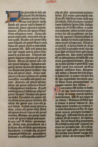
Figure 1: The first page of the Gospel of Matthew of the New Testament kept at the Universidad de Sevilla, from were the letters that we compare were taken.

We have chosen for convenience the first page of the Gospel of Matthew (see Figure 1) and we have considered in that page 10 letters i and 21 letters a. The quantity of 10 objects is small enough to permit the computation of the optimal clustering under any prefixed criterion, by simple exhaustive search. On the other hand, 21 objects allow to find out more classification patterns, although we must resort to an approximate method of cluster analysis because of the enormous time that the full enumeration would take.

The paper is organised as follows: In Section 2 we introduce our main mathematical tools, cluster analysis and outlier testing, recall some basic concepts of classical typography, and briefly highlight the facts that confer its importance to the book under consideration. Section 3 is devoted to the detailed description of the procedure followed to measure the distances between pairs of printed letters, which is the initial datum to apply the cluster analysis. Section 4 explains our exact method to find a good clustering and its application to 10 letters i in Matthew’s first page; exact means that an optimality criterion is established and that the absolute optimum is found with respect to that criterion. The approximate cluster analysis is described in Section 5, and it is illustrated with letters i one more time. The results are compared to those obtained with the exact method; this comparison will permit us to ensure that the approximate method applied to the twenty-one letters a in the next Section 6 is meaningful. The actual application of the hierarchical clustering is done in Subsection 6.1, whereas in 6.2 we apply a statistical method of detection of anomalous data (outliers) to validate the clusters obtained in 6.1.

It is not possible to represent graphically each letter as a point in some space, in such a way that the ordinary Euclidean distances among the points coincide exactly with the measured distances, since the latter are not true distances in the mathematical sense (the triangle property does not hold true). However, it is possible to represent the relative positions of the letters approximately, in 2 and 3 dimensions, by means of the so-called Multidimensional Scaling. In Section 7, a representation is the plane is given for both letters. The final Section 8 sketches the future plans in the line of research of this paper.

The present study has a necessary conservative bias. We are asking the experimental data to give us more than circumstantial evidence of the existence of several concurrent matrices, since this is a conclusion that runs against the currently accepted theory.

2 Preliminaries

2.1 Mathematical tools

Cluster analysis comprises a variety of methods that intend to obtain a reasonable grouping of a set of objects, based on the similarities among them. Each group is called a cluster, and a particular grouping, where each object is assigned to one cluster, is called a clustering. In modern statistics, cluster analysis is viewed as the main tool in the field of unsupervised learning.

To perform a cluster analysis it is enough to have a measure representing a “distance” or dissimilarity between each pair of objects. Ideally, a cluster must possess internal cohesion (i.e. small dissimilarities among the objects of the same cluster) and external isolation (that means, large dissimilarities between two objects of different clusters). There are several reasonable ways to implement this idea. The choice of one or another is a matter of mathematical modelling, and must be done to suit the particular situation at hand. In Subsection 4.2 we explain different good standard possibilities and justify our specific choice, which is in fact a variant of one of them, and seems to be new.

Cluster analysis will be complemented, in the study of letters a, with two additional tools. On the one hand, we will use the data supplied by a small set of letters printed with brand new types cast with the same matrix. This set will play the role of control group to estimate which sort of variability one can expect from letters with a common matricial origin (Subsection 6.1). On the other hand, we will use statistical tests for the detection of extreme data (outliers) to confirm, with a probability of error controlled and small, that two different clusters must be indeed considered distinct (Subsection 6.2).

A classical exposition of cluster analysis can be found for instance in Gordon [7]. A modern approach, imbedded in the so-called unsupervised learning theory, is Chapter 14 of Friedman–Hastie–Tibshirani [6]. The basic reference on outliers is the book by Barnett and Lewis [3].

2.2 Typographical terms

For the reader not well acquainted with the concepts of classical (i.e. non-digital) typography, we briefly explain some terms and procedures here. They are not strictly needed to follow the rest of the article, but they help in understanding the motivation of our work. For a detailed and illustrated description, we refer the reader to Smeijers [11].

A matrix is a piece of brass or copper in which the letter is engraved, by means of a previously made steel tool called a punch, which represented the character in reverse. One punch is needed for every character of a typeface and every size. Some parts of the punch are actually made by means of a counterpunch, but we do not need to go that far here.

The matrix already contains information on the height (point size) of the printed character, but the space that the metal type will really occupy in the line (the character width) is not yet determined. The type itself is cast from the matrix and a mould in an alloy of lead. There is one degree of freedom in the position of the mould, which determines the character width. In the matrix, the character has the right-reading direction, but it is engraved. In the type it shows in the wrong-reading direction and in relief.

The types are then gathered in a form to print a whole page. Several types of each character are therefore needed at the same time to compose a page.

The precise methods used by Gutenberg are still the subject of much research, but, according to [2], the method described here was well established by 1470.

2.3 The 42-line bible

The printing of the so called 42-line bible started in 1453 and was a very serious enterprise at that time. Gutenberg had been working for years perfecting the foundry mould technique with his previous metallurgical knowledge, and he needed the aid of the businessman Johannes Fust to finance the project, and the collaboration of the calligrapher Peter Schöffer to develop the typographical concept. The society was broken in the middle of the production of the approximately 200 copies of the book, and Gutenberg was removed from the project and sued by Fust. The whole printing was completed in August 1456.

There were other minor printing works before and after this one, and several versions of the same manuscript are named, when possible, according to the number of lines per page. The B42, however, possess several pages printed at 40 lines, and it is not yet clear what was the reason. It is anyway considered the start of an era, because of the huge dimension of the work. Moreover, all copies show still today an extremely beautiful and bright ink, made from a recipe that has been lost, and that was never used again in subsequent work. Chemical non-destructive analysis carried out in the 1980’s (Cahill-al. [9]) have found out a high metallic content, especially of lead and copper, but the compounds used and their proportions are not known.

All these facts have contributed to make this bible one of the most interesting books of all times, from many scientific, social and historical points of view. Currently, around 55 copies are known to have survived either totally or partially. An inventory can be found in the fundamental work of Paul Schwenke [10]. For a general history of the book, we recommend [5].

3 How the dissimilarities were measured

Although we will use both terms distance and dissimilarity, we recall that the dissimilarities here need not respect the triangular inequality, hence they are not distances in the usual mathematical sense.

The measuring device was the Mitutoyo QVA-200 [8], with a resolution of 0.0001 mm, and equipped with its proprietary software QVPack and FormPack. The letters were measured from a back up microfilm of the New Testament of the 42-line bible located in the library of the Universidad de Sevilla [1].

To estimate the measurement error attributable to the device and the measuring process, we measured the dissimilarity of one scanned letter with itself, and the values were in the order of $10^{-27}$ mm². Two different scans of the same letters gave rise to a value of at most $10^{-6}$. As we will see, this value is at least one order of magnitude below the relevant values in measuring the dissimilarities between two different printed letters, and therefore the measuring process can be considered stable and trustable in this aspect. This process is subsequently described.

The measuring device scans each printed letter and determines the contour of its shape. A contour is approximated by points and by line segments joining the points, forming a polygonal closed curve. Some letters possess empty inner spaces (counters), and in this case the contour is constituted by more than one connected curve.

The first step in the measuring process of two given contours $A$ and $B$ is to place them in a coordinate plane, in a similar orientation and sharing a common reference point, e.g. the barycenter. Then an initial distance between the two shapes is determined and one of the shapes is moved in the plane (with translations and rotations), in order to obtain a lower distance. The distance is again computed and a new movement takes place. This iterative process stops when no further improvement seems possible.

At each iteration $n$, the distance is computed in the following way: From each point $p$ of contour $A$, its Euclidean distance $d(p,B)$ to contour $B$ is computed, that means, the distance to the closest segment of contour $B$. The squares of the distances are then added up:

$$D_{n}(A,B):=\sum_{p\in A}d(p,B)^{2}$$

If the process stops after $n_{f}$ iterations, the value $D_{n_{f}}$, divided by the number of points in $A$, is taken as the dissimilarity $D(A,B)$ of $A$ with respect to $B$. Since the role of both shapes in this process is not symmetric, the roles are interchanged and the corresponding quantity $D(B,A)$ is computed. The final (symmetric) value of dissimilarity between $A$ and $B$ will be the mean

$$\mbox{\rm diss}(A,B):={\textstyle\frac{1}{2}}\big{(}D(A,B)+D(B,A)\big{)}\ .$$

The division by the number of points of the shape allows to compare different pairs of shapes in a common scale.

4 Exact clusterings for letter i

4.1 Dissimilarity table

The 10 letters i printed in the odd numbered lines in the first page of the Gospel of Matthew have been compared in pairs with the procedure described in Section 3, and a symmetric table of dissimilarities has been obtained. This is the suitable initial datum to proceed with the cluster analysis.

The original dimensions of the letters in the microfilm are in the orders of $10^{-1}$ mm (the ’x’ height is around 0.285 mm), and give rise to dissimilarities in the order of 10^-5 mm². For a more comfortable visualisation of the values, these have been multiplied by $10^{4}$, and the leading zeroes are omitted. The results are depicted in Table 1.

	i1	i2	i3	i4	i5	i6	i7	i8	i9	i10
i1		.2329	.3518	.2310	.1912	.3213	.2179	.2652	.2590	.3929
i2	.2329		.2097	.0283	.0701	.0801	.1139	.0425	.0835	.0907
i3	.3518	.2097		.1750	.1638	.3713	.0670	.1901	.1232	.3290
i4	.2310	.0283	.1750		.0895	.0756	.0902	.0512	.1026	.0926
i5	.1912	.0701	.1638	.0895		.1541	.1219	.1285	.1028	.2014
i6	.3213	.0801	.3713	.0756	.1541		.1467	.0560	.1324	.0645
i7	.2179	.1139	.0670	.0902	.1219	.1467		.0977	.0900	.2186
i8	.2652	.0425	.1901	.0512	.1285	.0560	.0977		.0718	.0719
i9	.2590	.0835	.1232	.1026	.1028	.1324	.0900	.0718		.1717
i10	.3929	.0907	.3290	.0926	.2014	.0645	.2186	.0719	.1717

Table 1: Dissimilarity table for the i

In the next subsections, we will study the classification of the letters i starting from this table. At the same time, we introduce the necessary cluster analysis theory. The code to perform the statistical analysis have been written in the language R [12].

4.2 How to value each possible clustering

As mentioned in Section 2, we intend to have cohesive and isolated clusters. Suppose we have $N$ objects (in our case, the $N=10$ letters i), and assume that we want to divide these objects into a given number $K$ of clusters. (Actually, we do not want to fix the number of clusters from the start, but let us assume that we do. Later we come back to the discussion on the number of clusters.)

In order to find the best clustering with $K$ clusters, we need to assign to each such clustering a certain cost, and then try to find the clustering with the minimum cost. There are several reasonable possibilities to translate the desired properties of cohesion and isolation into a cost function.

Common criteria proceed by evaluating the cost of each specific cluster and then combine the individual costs of the clusters. Both things can be done in several ways. For the first one, the following values are typically used:

1. The maximum of the dissimilarities among objects in the cluster.

2. The sum of those dissimilarities.

3. For each object, the sum of all dissimilarities between the object and the remaining ones are measured. Among all these quantities, the smallest one is chosen.

Valuations based in the minimum or the sum of dissimilarities between objects in the cluster and objects not in the cluster are also used.

We will use a variant of criterion 3, whose justification will be seen later:

1. For each object, the mean of all dissimilarities between the object and all other objects in the cluster is measured. Among these quantities, the smallest one is taken.

To combine the costs of each individual cluster, there are also two usual criteria:

1. Adding up the costs of all clusters.

2. Taking the maximum of the costs.

Methods 3 and 4 have the advantage that they distinguish a particular object in each cluster, namely the one for which the sum or mean of dissimilarities with the other objects is smallest (the same object in both methods, obviously). This allows to see the other objects as located “around the privileged one”. In our case, it allows to take one letter as a “model” and to think of the other ones as “variants” of the model, representing, in theory, a printed letter coming possibly from the same matrix as the model but with different metal types and printing errors.

Between possibilities (a) and (b), we prefer the second, because with the first we may find clusters with a high cost coexisting with clusters of small cost. Taking the maximum as the value to minimize tends to make the clusters uniform in this sense, and in our opinion this is more reasonable and conservative in the situation we are studying.

Once we decided to use criterion (b) for the combination of the costs of all clusters, the new proposed alternative 4 is better than the standard idea 3, as the next example shows: Suppose that for the letters i we want to compare clustering

$$\{1\}\ \ \{2,3,4,5,6,7,8,9,10\}\ ,$$

with clustering

$$\{1,10\}\ \ \{2,3,4,5,6,7,8,9\}\ .$$

With the combination 3-b, the first one has a cost of 0.7050 and the second one a cost of 0.6124, therefore making the second option preferable. But this does not seem reasonable, because letters 1 and 10 are the farthest apart in the whole set. What happens here is that in the first clustering we have a cluster of zero cost (because there is only one object in it, so that the internal cohesion is absolute) and another one with cost 0.7050; in the second clustering, the first cluster new cost is 0.3929, the distance between letters 1 and 10, and the second lowers to 0.6124. The maximum has therefore dropped from 0.7050 to 0.6124, and the second clustering turns out to be better.

This inconvenience tends to appear with criteria 3-b whenever we have clusters with a very unbalanced quantity of elements. With the alternative 4-b, the number of elements in the clusters is not relevant. In the same example, now the first clustering has a cost of 0.0881, much better than the second, which is 0.3929.

In summary, we take combination 4-b as the best suited for this study, although we have not been able to find in the literature an example of application of this particular combination of criteria. Our choice gives rise to:

• The possibility of graphically representing the clusters as stars, with a model letter in the center, and the other letters around, as variants of the model.

• No coexistence of very cohesive clusters together with clusters with little cohesion.

• No coexistence, within a cluster, of letters distant from the center of the star, together with letters close to it.

4.3 Finding the optimal clustering

When the number of objects is small, and still assuming that we have fixed the number of clusters, the optimal clustering can be found by exhaustive enumeration of all possible clusterings.

We have used this direct method to classify the 10 letters i in $2$ and $3$ clusters. From the 511 possible partitions into two clusters, the best one is

$$\{1\}\ \ \{2,3,4,5,6,7,8,9,10\}\ ,$$

whereas among the 9330 clusterings with three clusters one finds

$$\{1\}\ \ \{3,7\}\ \ \{2,4,5,6,8,9,10\}\ .$$

As mentioned above, it is possible to graphically represent these clusterings by means of “stars”. The best clustering with three clusters is so displayed in Figure 2. Letter i1 is isolated, letters i3 and i7 form a second cluster, in which it is irrelevant which letter is taken as the center, and finally the remaining letters form a cluster around letter i2. The distances from i2 to its companion letters are shown on the solid lines, and the distances with the other three letters are also shown, on half-dashed lines. (The lengths of the lines in the picture are not proportional to the dissimilarity.)

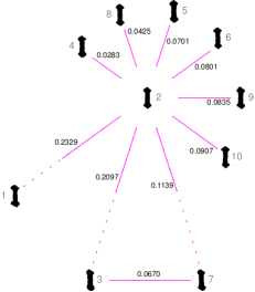
Figure 2: A star-shaped representation of the best clustering with three clusters. The objects are reproductions of the actual letters scanned.

Notice that the internal distances are smaller than the distances among model letters of the different clusters. This is not a necessary consequence of the criterion chosen, but and additional good property enjoyed by this particular clustering.

We could have tried to find the best clustering with four or more clusters, but there are very few objects, and its validity would be questionable. At the end of Subsection 6.2 we give another reason against the possibility of more than three clusters.

For the 21 letters a, the direct and exact method was not computationally feasible, and we resorted to and approximate method, as we will see in Sections 5 and 6.

4.4 The number of clusters

The issue of the number of clusters present, or of the existence of more than one, does not have a universal solution. Our point of view is based in the following considerations:

• First of all, we want to be in the conservative side; that means, we prefer to err by ascribing two letters to the same matrix when they actually come from different matrices, than to err by saying that they come from different matrices when they in fact have a common origin.

• Secondly, our goal is not to determine exactly how many distinct matrices were used (even in only one page). We only want to decide if there is enough evidence that there were more than one, or more than two, etc.

• In the third place, although it is necessary to take some decisions a priori that may influence the result (choosing a criterion for what is an optimal partition, or choosing the approximate method to employ), then, consistently with the conservative philosophy, the clusters are reexamined with an additional criterion to ensure its isolation (see Subsection 6.2).

5 Approximate clusterings

To compute the best partition into clusters, there is no way essentially more efficient than the exhaustive enumeration that we have applied to letters i. Therefore, if the enumeration is impossible because of the input size, one has to settle for some approximate method, able to provide a reasonably good solution.

The approximate method that we use here corresponds to the heuristic procedure called agglomerative hierarchical clustering (see, e.g. [6], [7]). With this method, one constructs in fact a hierarchy of clusterings, so that one has to decide afterwards which clustering in the hierarchy to keep.

It starts by declaring each object as a cluster by itself and then bigger clusters are constructed from smaller ones in sequence. At each step, two clusters are merged together to form a bigger one, namely, those which are the closest in some sense.

This idea raises the need to define a notion of dissimilarity among clusters, which involves again a certain arbitrariness in the choice. There are three reasonable and commonly used possibilities:

1. The dissimilarity between two clusters is the dissimilarity between their most similar objects. (This option is known in the literature as single linkage.)

2. The dissimilarity between two clusters is the dissimilarity between their most distant objects (known as complete linkage).

3. The dissimilarity between two clusters is the arithmetic mean of the dissimilarities between the objects in both clusters (called average linkage).

We illustrate the hierarchical agglomerative clustering arising from the three possibilities above with the letters i, already studied with an exact method, and we discuss the correlation of each variant with respect to the exact results. We are able in this way to justify the choice of the next section for the study of the 21 letters a.

5.1 The single linkage

With any of the three possibilities one can draw a graphical representation of the agglomerative process, called dendrogram. For instance, the single linkage for the 10 letters i produces the dendrogram of Figure 3. The height of the horizontal lines, read in the vertical axis, is the distance between the two clusters that hang from the line, and that combine into one at that point.

Now, looking at the dendrogram, we should decide how many and which clusters seem to exist. When applying the method to the letters a, we will use additional information to help us in this purpose. Here, we only want to observe to which extent the approximate methods give similar results to the exact method used in the previous section.

Specifically, we see in the dendrogram that letter 1 must be clearly set apart from the others, and we also observe a clear separation between group $\{3,7\}$ and the remaining letters, although not so clear as with letter 1. This reflects fairly well in a graphical way the results that we obtained when we imposed 2 or 3 clusterings. Moreover, looking for a splitting in more than three clusters will not be supported by the dendrogram.

The single linkage method is very conservative, in the sense that it can easily consider in the same cluster two very distant objects, as long as they are connected by a chain of other objects, each one similar enough to the next.

5.2 The complete linkage

The complete linkage method takes the opposite heuristic and this makes it little conservative: It tends to keep separated pairs of objects that perhaps are not so different. The clusters produced tend to be cohesive but not quite isolated.

With the complete linkage agglomerative clustering we obtain the dendrogram in Figure 4. Up to four clusters could be concluded from the picture. Moreover, even sticking to three clusters, the result would not coincide with that of the single linkage (letters 5 and 9 switch clusters). This dendrogram thus suggest a result more distant to the exact one than that obtained with the single linkage method.

5.3 The average linkage

The average linkage is half-way between the previous methods. It gives rise to dendrogram of Figure 5. The distance between two clusters $C_{1}$ and $C_{2}$ is computed as

$$\frac{1}{|C_{1}|\cdot|C_{2}|}\sum_{o_{1}\in C_{1}}\sum_{o_{2}\in C_{2}}\mbox{\rm diss}(o_{1},o_{2})$$

where $|C|$ means the number of elements of cluster $C$, and $\mbox{\rm diss}(o_{1},o_{2})$ is the given dissimilarity between objects $o_{1}$ and $o_{2}$.

The following list indicates the order in which the clusters are formed, and the distance between merging clusters. The central column indicates which clusters are merged. A number n refers to a single object (the n-th letter i), whereas a letter means the multiobject cluster formed in the line labelled with that letter.

	merge	distance
a	2 -- 4	0.0283
b	8 -- a	0.0469
c	6 -- 10	0.0645
d	3 -- 7	0.0670
e	b -- c	0.0778
f	5 -- 9	0.1028
g	e -- f	0.1205
h	d -- g	0.1744
i	1 -- h	0.2737

We observe that the dendrogram here looks more correlated with the exact result of Section 4 than the complete or even the single linkage dendrogram. The clearest cut point produce the same partitions in two and three clusters and, moreover, the separation of the group $\{3,7\}$ is more apparent here. Therefore we believe that this method is the one with results more similar to the exact method corresponding to criterion 4-b that we have applied. We will adopt it for the classification of the twenty-one letters a in the next section.

Figure 3: Dendrogram for letter i with the single linkage method

Figure 4: Dendrogram for letter i with the complete linkage method

Figure 5: Dendrogram for letter i with the average linkage method

6 Cluster analysis for letter a

In the previous Section 5, we have compared several approximate clustering methods with the exact cluster analysis performed with our optimality criterion. We concluded that the average linkage method was the one with the best results. We thus apply this method to classify the twenty-one a taken from the first page of the Gospel of Matthew. The corresponding dissimilarity measures can be seen in Table 2.

	a1	a2	a3	a4	a5	a6	a7	a8	a9	a10	a11	a12	a13	a14	a15	a16	a17	a18	a19	a20	a21
a1		.1277	.1165	.1892	.1338	.1196	.1301	.1536	.1049	.1741	.2653	.2509	.3712	.1489	.1315	.2345	.1866	.1375	.1939	.0868	.2262
a2	.1277		.1160	.2370	.1543	.1391	.1173	.1347	.1617	.1643	.2845	.1522	.2817	.1422	.1464	.1169	.1114	.1723	.1861	.1834	.1606
a3	.1165	.1160		.1668	.0769	.1119	.1474	.1353	.1471	.2447	.2214	.2015	.3191	.0990	.0897	.1919	.1715	.1186	.1720	.0958	.1771
a4	.1892	.2370	.1668		.1468	.1637	.2363	.3173	.1133	.3779	.3533	.4261	.5766	.2478	.1402	.3280	.2332	.2330	.2460	.1057	.3028
a5	.1338	.1543	.0769	.1468		.1128	.1026	.1214	.1395	.2114	.2070	.2094	.3265	.1582	.0906	.1677	.1749	.0940	.1252	.0964	.1563
a6	.1196	.1391	.1119	.1637	.1128		.1256	.1274	.1184	.1778	.2264	.2161	.3179	.1294	.0754	.1651	.1132	.0938	.1834	.1421	.1254
a7	.1301	.1173	.1474	.2363	.1026	.1256		.1131	.1669	.1856	.1928	.2188	.3023	.1735	.1425	.1223	.1489	.1190	.1161	.1835	.1296
a8	.1536	.1347	.1353	.3173	.1214	.1274	.1131		.2087	.1327	.1907	.1179	.2089	.1105	.1108	.0972	.1221	.1289	.1721	.2228	.1041
a9	.1049	.1617	.1471	.1133	.1395	.1184	.1669	.2087		.2454	.3359	.3063	.4550	.1769	.1224	.2264	.1415	.1986	.2144	.1320	.2119
a10	.1741	.1643	.2447	.3779	.2114	.1778	.1856	.1327	.2454		.2371	.1281	.1843	.1964	.2129	.1809	.1558	.1694	.3145	.3417	.2009
a11	.2653	.2845	.2214	.3533	.2070	.2264	.1928	.1907	.3359	.2371		.2189	.2366	.1738	.2451	.1890	.2468	.1972	.2894	.3544	.2449
a12	.2509	.1522	.2015	.4261	.2094	.2161	.2188	.1179	.3063	.1281	.2189		.1226	.1593	.2342	.1295	.2077	.2282	.2843	.3288	.1815
a13	.3712	.2817	.3191	.5766	.3265	.3179	.3023	.2089	.4550	.1843	.2366	.1226		.1923	.3397	.2185	.2995	.3113	.5016	.5017	.2912
a14	.1489	.1422	.0990	.2478	.1582	.1294	.1735	.1105	.1769	.1964	.1738	.1593	.1923		.1444	.1752	.1514	.1907	.2673	.1665	.1432
a15	.1315	.1464	.0897	.1402	.0906	.0754	.1425	.1108	.1224	.2129	.2451	.2342	.3397	.1444		.1586	.1224	.1159	.1655	.1307	.1629
a16	.2345	.1169	.1919	.3280	.1677	.1651	.1223	.0972	.2264	.1809	.1890	.1295	.2185	.1752	.1586		.1392	.1809	.1737	.2762	.1106
a17	.1866	.1114	.1715	.2332	.1749	.1132	.1489	.1221	.1415	.1558	.2468	.2077	.2995	.1514	.1224	.1392		.1881	.2208	.1880	.1372
a18	.1375	.1723	.1186	.2330	.0940	.0938	.1190	.1289	.1986	.1694	.1972	.2282	.3113	.1907	.1159	.1809	.1881		.1668	.1922	.1545
a19	.1939	.1861	.1720	.2460	.1252	.1834	.1161	.1721	.2144	.3145	.2894	.2843	.5016	.2673	.1655	.1737	.2208	.1668		.1756	.1438
a20	.0868	.1834	.0958	.1057	.0964	.1421	.1835	.2228	.1320	.3417	.3544	.3288	.5017	.1665	.1307	.2762	.1880	.1922	.1756		.2233
a21	.2262	.1606	.1771	.3028	.1563	.1254	.1296	.1041	.2119	.2009	.2449	.1815	.2912	.1432	.1629	.1106	.1372	.1545	.1438	.2233

Table 2: Dissimilarity table for the a

6.1 Dendrograms for letter a

The dendrogram corresponding to the average linkage variant of the hierarchical clustering is displayed in Figure 6.

The order in which the different clusters are sorted horizontally does not have any special meaning. Here we follow the convention of drawing to the left the more compact cluster, that is, the one formed at the lowest level. The corresponding sequence of cluster formation, sorted by merging level, is given in the following list. We follow the same convention of the analogous list above.

	merge	distance
a	6 -- 15	0.0754
b	3 -- 5	0.0769
c	1 -- 20	0.0868
d	8 -- 16	0.0972
e	a -- b	0.1012
f	18 -- e	0.1056
g	21 -- d	0.1074
h	2 -- 17	0.1114
i	4 -- 9	0.1133
j	7 -- 19	0.1161
k	12 -- 13	0.1226
l	c -- f	0.1296
m	g -- h	0.1351
n	14 -- m	0.1445
o	i -- l	0.1506
p	10 -- k	0.1562
q	j -- n	0.1640
r	o -- q	0.1752
s	11 -- p	0.2309
t	r -- s	0.2584

Figure 6: Dendrogram for letter a with the average linkage method

Concerning the choice of the clustering in the hierarchy, which amounts to determine the number of clusters, the usual heuristic, when no other information is available, is to “cut” the dendrogram wherever the jumps in the distances of consecutive mergings are higher than a threshold magnitude. For instance, the jump from 0.1752 to 0.2309 between lines r and s would give us a partition in three clusters that looks quite clear.

But we do have an additional information to determine the number and composition of clusters. This information is given by a set of dissimilarities measured from a test printing of newly created types. We have used types belonging to the typographic collection of the Bauer Neufville Type Foundry, kept at the Universitat de Barcelona. These will play the role of “control group”, since we know for sure that they come from the same matrix. If we try to divide them in clusters, all of them must therefore become members of the same and only cluster. Comparing these letters in the same way as we did with the microfilmed letters of the Gospel of Matthew, we can see the magnitude of the dissimilarities that we can expect and that are attributable only to the errors of construction of the metal types and to printing errors.

The actual size of the types of the control group is of course different from the one of the microfilmed letters, so that the absolute values of the dissimilarities cannot be directly used to compare the two groups. We have to define a common comparison base that will not be influenced by the different size. A natural and easy way to establish a common unit of measure is the following:

1. The control group is organised around a model letter, with the same procedure used with letters i in Section 4 (all of them in the same cluster, obviously), obtaining a set of distances to the model.

2. The quotient is computed between the largest and the smallest distance to the model, as a measure of dispersion of these distances, which is a value independent of the units of measure.

We have applied this procedure to the letters m, i, a, o, with five specimens each, and the results are summarised in Table 3.

	distances to model	mean	max/min
m	5.9731, 3.9409, 5.5055, 3.9967	4.8540	1.5156
i	3.2364, 5.9557, 2.8876, 3.9188	3.9996	2.0625
a	7.4534, 4.8179, 4.6993, 3.7450	5.1789	1.9902
o	1.7965, 1.8714, 2.0286, 1.7940	1.8726	1.1307

Table 3: Distances obtained with brand new metal types, and five specimens per glyph

The quotient between the largest and the smallest distance to the model gives us an estimate of the variability that we can expect from a unique matrix. We see that the quotients range between 1.1307 and 2.0625.

We will use this estimate in the following way for our set of a: We take the two letters which are the closest and declare them, obviously, as belonging to the same cluster. This minimum distance is 0.0754, and it is found between letters a6 and a15. According to the data obtained from the control group, the letters at a distance up to 2.0625 times this minimum distance (i.e. distances up to 0.1555) may perfectly belong to the same cluster.

Therefore, we can draw a cutting line in the dendrogram at level 0.1555 (the red line in Figure 6), and declare all clusters grouped below this line as indivisible.

Thus, we obtain six clusters. We can now construct the stars corresponding to these clusters, finding their model letters and the distances from the remaining letters to its model (see Table 4).

	cluster	model	mean of distances	minimum, maximum	max/min
1	{4,9,1,20,18,6,15,3,5}	5	0.1114	0.0769, 0.1468	1.9090
2	{7,19}	7, 19	0.1161
3	{14,21,8,16,2,17}	8	0.1137	0.0972, 0.1347	1.3858
4	{11}	11	-
5	{10}	10	-
6	{12,13}	12, 13	0.1226

Table 4: Preliminary clustering for letter a

Our conclusion up to this moment is that the maximum number of clusters that we obtain from the twenty-one letters a is six, because splitting any one of them would be analogous to declare that the metal types of the studied control group came from more than one matrix, which is false.

6.2 Validation of clusters

We are now interested in checking if we have actually gone too far in the number of clusters found, and some of them should better be merged into larger ones, following our conservative criterion to declare two letters as coming from the same matrix if there is no strong evidence against this hypothesis. Take also into account that the dendrogram is the result of an approximate method, built upon a somewhat arbitrary choice of the criterion with which the hierarchy is constructed; it is therefore absolutely necessary to validate the present clusters with some sieve reflecting the conservative spirit.

To this end, we use a statistical test for the detection of outliers. In general an outlier in a set of numerical data is a datum markedly different from the rest, that seems to result from some sort of measuring error or typo, or in summary that should not be there, because it does not really belong to that data set.

As an example, let us take cluster number 3. The model is letter a8 and so we can draw a star with center in a8 and the corresponding distance to the other letters. These distances are, sorted in increasing order:

0.0972 0.1041 0.1105 0.1221 0.1347

Take now any other letter, not belonging to cluster 3, and observe its distance to the model a8. For instance, a1 happens to be at a distance 0.1536 from a8. Is this distance too large to include also a1 in cluster 3? Or, on the contrary, it is not much different from the others, and the larger distance is only the product of chance?

The conservative hypothesis, and therefore the one that it is considered true a priori, as in any statistical test, is the second possibility above: the distance between a1 and a8 is not exceedingly large and in consequence a1 should also belong to cluster 3. This null hypothesis will be abandoned only if there is enough evidence against it. The evidence is measured in terms of the $p$-value, the probability of rejecting the null hypothesis when it was in fact true. If the $p$-value is less than a certain threshold fixed beforehand (typically 10%, 5% or 1%), then the null hypothesis is rejected; otherwise, it is kept, conservatively, as the good one (albeit with a probability to err with this conclusion that can be very high).

We are going to apply the so-called Dixon’s test, the usual one to test for the presence of one outlier in a data set. Let $x_{1},\dots,x_{n}$ be the data set, sorted in increasing order, including as $x_{n}$ the suspect datum. Dixon’s test computes the statistic

$$Q:=\frac{x_{n}-x_{n-1}}{x_{n}-x_{1}}\ .$$

Intuitively, a large value for this quotient indicates that there is a large difference between the last value and the one before last (relatively to the dispersion of the whole data set), inducing us to believe that the last value is an outlier and to reject the working hypothesis. If, on the contrary, the quotient is small, then the difference between $x_{n-1}$ and $x_{n}$ is small and there is no reason to declare $x_{n}$ as outlier.

Continuing the example above, if we want to see if letter a1 belongs to cluster 3, we compute the value of the Dixon’s statistic:

$$Q=\frac{0.1536-0.1347}{0.1536-0.0972}=0.3351\ .$$

In order to apply reliably Dixon’s test to determine if the value 0.3351 is too large or not, the data must satisfy two assumptions that in our case are fulfilled:

1. The data follow a Gaussian law, and

2. they are statistically independent.

Gaussianity is justified by the fact that each datum is the sum of a large quantity of very small values (the distances from points of one contour to segments of the other, divided by its number, see Section 3). Therefore, independently of the underlying probability law of those small values, the sum will very approximately follow a Gaussian law, thanks to the Central Limit Theorem.

The independence is obvious because the result of measuring the distance form any letter to the “model” letter does not influence the result of the distance between a third letter and the model. (Notice that if we include the distance among the letters which are not models, the independence would be lost.)

Under these conditions, the probability distribution of the random variable $Q$, assuming that there are no outliers, is known. This allows to compute the probability that $Q$ attain a value greater than or equal to the observed one if $x_{n}$ is not an outlier. In the case of our example, the probability of the event $\{Q\geq 0.3351\}$ is approximately 0.27. This is the probability of mistakenly declare that $x_{n}$ is an outlier. Of course, it is too high to take the risk.

Letter a1 may therefore be included in cluster 3. But we have said that cluster 1 will not be split. So, let us check what happens with the remaining letters in cluster 1, namely a4, a9 and a20, which are at distances 0.3173, 0.2087, 0.2228 from the model a8 of cluster 3 (see Table 2). Using Dixon’s test one finds that all three of them fall below the 5% threshold of probability of a mistake if we declare them outside cluster 3 ($<0.0001$, 0.0156, and 0.0095, respectively). So this is what we do and we keep definitively separated clusters 1 and 3.

Repeating the same idea with the remaining clusters, we obtain that:

• Cluster 5 integrates in cluster 6 (in fact, they were close to be already merged when we drew the horizontal line in the dendrogram).

• Cluster 2 can easily be integrated in cluster 1. In this case, both distances to the model a5 are even smaller than those of some other letters already included in cluster 1. Cluster 2 could also be integrated in cluster 3, but not so clearly, since the $p$-value for letter a19 is 0.0860, so that with the milder threshold of 10% as error probability it will not be integrated.

• Cluster 4 (letter a11) does not integrate in the new cluster union of 5 and 6 (letters a10, a12, a13), with $p$-value $0.0485$. Similarly, it cannot be integrated in the cluster union of 1 and 2 (with $p$-value $0.0193$), nor in cluster 3 ($p$-value $0.0332$). Thus letter a11 remains alone definitively.

• It can be checked that there are no other possibilities for merging the new clusters among them.

We arrive then to the final classification in four clusters given in Table 5.

	cluster	model	mean of distances	minimum, maximum	max/min
A	{4,9,1,20,18,6,15,3,5,7,19}	5	0.1114	0.0769, 0.1468	1.9090
B	{14,21,8,16,2,17}	8	0.1137	0.0972, 0.1347	1.3858
C	{11}	11	-
D	{10,12,13}	12	0.1254	0.1225, 0.1281	1.0457

Table 5: Final classification in clusters for of letters a

We remark once again that the procedure we have used is conservative: we are pretty sure that there is more than one cluster (four at least) in the 21 letters a studied, but it is perfectly possible that there are actually more than 4.

We also remark that sometimes an outlier can be masked by the presence of another questionable datum. There exist statistical tests to expose the existence of two outliers at once (e.g. Grubbs’ test, see [3]); however, following our conservative spirit, we have preferred not to try to identify such situations and, if it happens, to accept both data as genuine.

At first sight, the decision of declaring as separate two clusters when just one of the letters of the first cluster is rejected as admissible by the second one may seem more risky. But one should take into account that it is still more risky to split a cluster which has been first declared indivisible. Suppose, on the other hand, that we do not want to split the first cluster but we want to know if it should be completely integrated in the second. Recall that this must be the null hypothesis of the test. Now, the probability of error in declaring mistakenly out of a cluster more than one letter is still smaller than the probability of declaring out of the cluster each one of them. Therefore, if one of the letters does not exceed the fixed 5% of probability of error, a set of more than one letter will not exceed that value either.

The following are the computed probabilities that have allowed to conclude the final classification of Table 5 from the preliminary classification of Table 4, through Dixon’s test. For each possible destination cluster, we list the candidate letters, with the cluster to which they belong. Only the rejections ($p$-values less than 5%) are shown. $1\mathop{\cup}\limits 2$ and $5\mathop{\cup}\limits 6$ mean the union of these clusters, whose model letters turn out to be a5 and a12, respectively.

letter	from cluster	to cluster	$p$-value
10	5	1	0.0294
11	4	1	0.0368
12	6	1	0.0326
13	6	1	$<0.0001$
4	1	3	$<0.0001$
9	1	3	0.0156
11	4	3	0.0332
13	6	3	0.0155
20	1	3	0.0095
10	5	$1\mathop{\cup}\limits 2$	0.0146
11	4	$1\mathop{\cup}\limits 2$	0.0193
12	6	$1\mathop{\cup}\limits 2$	0.0167
13	6	$1\mathop{\cup}\limits 2$	$<0.0001$
1	1	$5\mathop{\cup}\limits 6$	0.0360
6	1	$5\mathop{\cup}\limits 6$	0.0500
7	2	$5\mathop{\cup}\limits 6$	0.0485
9	1	$5\mathop{\cup}\limits 6$	0.0250
11	4	$5\mathop{\cup}\limits 6$	0.0485
15	1	$5\mathop{\cup}\limits 6$	0.0416
18	1	$5\mathop{\cup}\limits 6$	0.0441
19	2	$5\mathop{\cup}\limits 6$	0.0284
20	1	$5\mathop{\cup}\limits 6$	0.0223

To close the section, we return for a moment to the analysis of the ten letters i, in connection with the validation of clusters.

In Section 4, we obtained the optimal (exact) clusterings, conditioned to the existence of exactly two or three clusters. We can also apply Dixon’s test for outliers to those clusterings, and the result confirms the partitions seen. It is also natural to use the test to check if a partition in 4 clusters could be reasonable. The result is negative:

The best clustering with four clusters (exact, with the criterion introduced in Section 4) is

$$\alpha=\{1\}\ ,\quad\beta=\{3\}\ ,\quad\gamma=\{5\}\ ,\quad\delta=\{2,4,6,7,8,9,10\}\ .$$

But Dixon’s test does not support i5 out of cluster $\delta$. It does for i1 and i3, with $p$-values $<0.0001$ and 0.0117, respectively.

The second best clustering with four clusters corresponds to

$$\alpha=\{1\}\ ,\quad\beta=\{3\}\ ,\quad\gamma=\{7\}\ ,\quad\delta=\{2,4,5,6,8,9,10\}\ .$$

which looks more consistent with our previous partition in three clusters. Again i1 and i3 cannot be integrated in $\delta$, with $p$-values 0.0032 and 0.0075 respectively, and, although i7 could be, we should integrate first i3, from the dendrogram, given that we cannot perform an outliers test against a cluster with one only element.

As a curiosity, it turns out that the model letters (center of the star) for clusters $\delta$ in the two cases above are different. They are i8 in the first case and i2 in the second. In fact, they are very close letters and these changes are not surprising when changing slightly the composition of a cluster.

In conclusion, this study forcing four clusters does not bring us more than what was already shown: We can postulate with confidence the existence of three clusters, and concerning its composition, the safest bet is our first option

$$\alpha=\{1\}\ ,\quad\beta=\{3,7\}\ ,\quad\delta=\{2,4,5,6,8,9,10\}\ ,$$

with a certain risk, coarsely bounded by a probability of 0.32 of error in separating letter 7 from cluster $\delta$. The clustering with two clusters, merging $\beta$ and $\delta$, looks to us extremely conservative.

7 Graphical representation of clusterings

The Multidimensional Scaling (MDS) is a technique that allows to represent graphically in dimensions 2 or 3 the set of objects that are being classified, providing a visual impression of the closeness among different objects or clusters of objects. The distances in the display are not the true dissimilarities; they are the best possible approximation (according to some loss function) so that the data can be embedded in the 2- or 3-dimensional space.

The specific coordinates of the points have no intrinsic meaning; only the relative position among objects are to be read. In particular, any rotation, symmetry or translation of the picture gives rise to another picture with exactly the same meaning. Yet it can be assured that the mapping is monotone: if an object possesses dissimilarities $d_{1}$ and $d_{2}$ with other two objects, and $d_{1}<d_{2}$, then the corresponding distances in the picture $\hat{d}_{1}$ and $\hat{d}_{2}$ also satisfy $\hat{d}_{1}<\hat{d}_{2}$.

The MDS in dimension 2 for the 10 letters i and the 21 letters a are shown in Figures 7 and 8. The stars of the optimal clustering found have also been displayed, and we see that the clusters appear quite clearly in the pictures.

Figure 7: MDS in dimension 2 for letter i

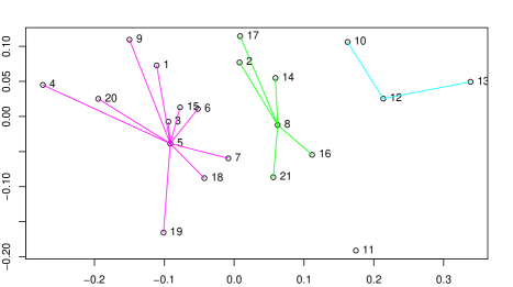
Figure 8: MDS en in dimension 2 for letter a

The extent to which a possible graphical representation of a set of objects differs from the real dissimilarities is called stress and can be defined in several reasonable ways. The representation used here corresponds to the variant known as Kruskal Non-metric Multidimensional Scaling. The stress $S$ is defined as

$$S=\sqrt{\frac{\sum(f(d_{ij})-\hat{d}_{ij})^{2}}{\sum\hat{d}_{ij}^{2}}}$$

where $d$ are the given dissimilarities among the objects, $\hat{d}$ are the distances in the graphic, and $f$ is a monotonically increasing transformation that gives an extra flexibility to the adjustment. The position of the points are obtained by seeking the distances $\hat{d}$ and the transformation $f$ that minimize the stress. The monotonicity of $f$ ensures that if one dissimilarity is smaller than another, then the corresponding distances in the picture preserve that order.

More details on Kruskal Non-metric Multidimensional Scaling can be seen, for instance, in Chapter 3 of [4], or in Chapter 11 of [13].

8 Conclusion and open questions

From the historical research viewpoint, finding out which tools were used or developed by Gutenberg and Schöffer to complete their monumental work is one of the most interesting items. The fact that metal types built from multiple matrices were used concurrently, as we prove here, is a new aspect that indicates that matrix construction was quite evolved. The use of punches and counterpunches to sculpt the inner contours is agreed today; the tools used for the outer contours are not so clear. The letters a, and other letters with counters, offer the additional possibility to shed light in this respect.

We have carried out a prospective study with the inner lower contour of letter a (in the gothic textura typeface it has indeed two inner contours), and the results seem to indicate that different outer contours combine with different inner contours. This may imply that punches were also used to delineate the external shape of the matrix. However, we feel that we should first gather many more experimental data, implementing also an improved measuring protocol, and we have therefore decided not to include those results here.

We have also started to measure letters coming from the subsequent pages of the same bible book, the Gospel of Matthew. We have computed their distances with the twenty-one letters of the first page, just to see if they can be integrated into the existing clusters or not. What we observe is that most of them integrate well in the clusters, but that a few new “models” appear. This was absolutely in line with what we expected after obtaining the results concerning the first page.

Notice that, using letters coming from different pages, and that may therefore be printed from the same metal type, three levels of similarity should be observed: Letters very similar among them, appearing for sure in different pages, printed with the same metal type; similar letters, but not that much, printed with different types but with a common matricial origin; and letters with low similarity, printed from types coming from different matrices. We do not have yet enough data to confirm this, but we believe it is feasible to carry out this programme in the future.

Acknowledgements. We thank Prof. Enric Tormo from the Universitat de Barcelona for his guidance in the historical aspects.

None of the authors is supported by any grant of the Spanish or Catalan governments.

References

- [1] Biblia Latina, [Moguntiae : Eponymous Typography (=Johannes Gutenberg)], ca. 1454 — August 1456 [Microfilm] Universidad de Sevilla, 2004.
- [2] Baines, P. and Haslam, A. Type & typography, Laurence King Publishing, London, 2002.
- [3] Barnett, V. and Lewis, T. Outliers in statistical data, Wiley, Chichester, 1984.
- [4] Cox, T.F. and Cox, M.A.A. Multidimensional scaling (2nd ed.), Chapman and Hall / CRC, Boca Raton, 2001.
- [5] De Hamel, C. The Book. A History of The Bible, Phaidon Press Inc., London, 1st edition, 2001.
- [6] Friedman, J., Hastie, T. and Tibshirani, R. The Elements of Statistical Learning, Springer, New York, 2001.
- [7] Gordon, A.D. Classification, Chapman and Hall / CRC, Boca Raton, 1999.
-
[8]
Machines de mesure par analyse d’image Mitutoyo [online]. France. ©2007.
http://www.mitutoyo.fr/
telechargement-catalogueue.php - [9] Schwab, R.N., Cahill, T.A., Kusko, B.H., Eldred, R.A., Wick, D.L. The Proton Milliprobe Analysis of the Harvard B42, Volume II, PBSA. 81:4, 403-432 (1987).
- [10] Schwenke, P. Johannes Gutenbergs Zweiundvierzigzeilige Bibel: Ergänzungsband zur Faksimile Ausgabe, Iminsel, Leipzig, 1923.
- [11] Smeijers, F. Counterpunch, Hyphen Press, London, 1996
- [12] The R Project for Statistical Computing [online]. Viena: The R Foundation for Statistical Computing. http://www.r-project.org .
- [13] Venables, W.N. and Ripley, B.D. Modern applied statistics with S (4th ed.), Springer, New York, 2002.
- [14] Zedler, G. Die Sogenannte Gutenbergbibel, XX, Verlag der Gutenberg-Gesellschaft, Mainz, 1929.