Controlling Effect of Geometrically Defined Local Structural Changes on Chaotic Hamiltonian Systems

Abstract

An effective characterization of chaotic conservative Hamiltonian systems in terms of the curvature associated with a Riemannian metric tensor derived from the structure of the Hamiltonian has been extended to a wide class of potential models of standard form through definition of a conformal metric. The geodesic equations reproduce the Hamilton equations of the original potential model through an inverse map in the tangent space. The second covariant derivative of the geodesic deviation in this space generates a dynamical curvature, resulting in (energy dependent) criteria for unstable behavior different from the usual Lyapunov criteria. We show here that this criterion can be constructively used to modify locally the potential of a chaotic Hamiltonian model in such a way that stable motion is achieved. Since our criterion for instability is local in coordinate space, these results provide a new and minimal method for achieving control of a chaotic system.

I Introduction

The issue of controlling chaos has attracted great interest in the last two decades; much work has been done in the case of dissipative systems. Ott, Grebogi and York (OGY) ott developed a method by which chaos can be suppressed by making small time-dependent perturbations in order to shadow one of the infinitely many periodic orbits embedded in the chaotic attractor. This method has been extended by many following studies kapitaniak ; dressler ; pyragas and successfully applied to experimental systems ditto .

As a result of the absence of attractors in conservative systems and the complex nature of the phase space combining regular and irregular regions, constructing an effective method has remained a challenging question. Lai Ding and Grebogi (LDG) extended the OGY method to Hamiltonian systems by incorporating the notion of stable and unstable directions at each periodic point.

In relation to the above question, Chandre et al. chandre ; chandre1 ; vittot have developed a method for constructing barriers in phase space to subdue chaotic behavior for large times. This method is based on the introduction of a specifically designed small control term which changes the dynamics from chaotic to regular behavior. Zhang et al. zhang have introduced a method for controlling chaos in two-dimensional Hamiltonian system which they called adaptive integrable mode coupling based on the separation of the system into two coupled subsystems one of which is stable and the other unstable; when the unstable system comes into the vicinity of the integrable system the conditions are reset resulting in an effective adaptive control. Cartwright et al. cartwright have constructed a method which permits stabilization of KAM islands through forward iteration of the orbits, and transforming them into global attractors of the embedded system. Ciraolo et al. ciraolo have used a method of adding a small perturbation to modify systems, such as nonlinear plasmas, to follow more regular motion. Additional efficient methods have been proposed in Kulp ; bolotin ; ding ; yugui ; zhihua ; some of these methods require tracking the trajectories while others involve the addition of interacting terms for which the criteria are somewhat sensitive.

Geometric approaches for the analysis of the stability of a given Hamiltonian have been widely discussed jacobi ; hadamard ; casettiReport ; casettiPRE ; cipriani ; BenZionPRL ; BenZionPRE1 ; BenZionPRE2 ; Kawabe ; szyd1 ; szyd2 ; szyd3 ; szyd4 , for which curvature of a manifold is associated with stability.

The pioneering work of Oloumi and Teychenné oloumi proposes a stabilization method by considering the Gaussian curvature of the potential energy as a source of chaos. Even if the condition of negative curvature of the potential and instability of the dynamics are not completely equivalent they were able to successfully control the instability by avoidance of negative curvature regions of the potential energy (ANCRP).

In this work we make use of a recently developed geometrical criterion BenZionPRL which is highly sensitive to instability in Hamiltonian systems, and has been shown to be in complete agreement with the results of the numerical technique of surface of section (Poincaré plot) and more effective than other geometric methods  BenZionPRE2 . This criterion is based on an equivalence between motions generated by Hamiltonian in the standard form with quadratic kinematic terms and additive potentials (which we shall call the Hamilton description) and a Hamiltonian in which the dynamics is described by a metric-type function of coordinates multiplying the momenta in bilinear form (which we shall call the Gutzwiller description) gutzwiller ; curtis ; moser ; eisenhardt ; arnold . The mapping between these equivalent descriptions was first introduced by Appel appell ; cartan ; landau ; zerzion . The criterion for stability developed in  BenZionPRL establishes an inverse mapping of the motion described completely geometrically in the Gutzwiller space back to the Hamilton description, carrying with it the covariance under diffeomorphisms that is a property of the Gutwiller dynamics. The resulting orbits in the Hamilton description, with the special choice of coordinates serving as the basis for the Appel type relation, reduce to the standard description of the Hamilton orbits under the Hamilton equations. In general geometric form, as geodesic equations, however, they are subject to analysis in terms of geodesic deviation, and the resulting formula can be reduced to a computation in the special coordinates of a new (symmetric) matrix valued criterion for stability BenZionPRL which has been shown to be very effective in a wide range of examples BenZionPRE1 ; BenZionPRE2 ; yahalom .

In the analysis of these systems, it was shown that the presence of negative eigenvalues for the stability matrix in the admissible physical region (for which $E>V$) results in a chaotic type Poincaré plot. Since the condition is local in coordinate space, the result necessarily implies some degree of ergodicity. There has, however, been no proof that the existence of negative eigenvalues is not strongly associated with the structure of the dynamics more globally, as is often the case, for example, for analytic function theory, where the presence of a complex pole implies a distortion of a relatively large region of the complex plane. The results of our application to the control of dynamical systems, however, indicates that the regions of negative eigenvalue correspond to a very localized phenomena. The observed instability they induce appears to be due to the passage of orbits through these regions, and they are not strongly correlated with the more global structure of the dynamics.

What we have done here is to identify the regions of negative eigenvalue in the coordinate space, and modify the Hamiltonian in these regions locally, removing the source of instability either by removing the instability inducing terms or varying the coupling to these terms to bring the Hamiltonian closer to an integrable form in these regions. The remaining part of the space is left to develop according to the full, nonlinear, symmetry breaking, evolution. The effect on the Poincaré plots, as we show here, is dramatic. This result provides strong evidence that chaotic Hamiltonian systems derive their properties from sources that may be thought of as highly localized in the regions of negative eigenvalues for the stability matrix. In addition to giving an interesting insight into the nature of Hamiltonian chaos, it also provides an effective control method in which the Hamiltonian dynamics is left to exercise its full function in a large domain of configurations, but is only constrained in prescribed local regions of the configuration space.

In the next section, we review the basic ideas underlying the geometrical criterion, and in the following section we give numerical results for the application of our control procedure for the cases of an oscillator with broken symmetry and a potential which may be derived from the Toda form.

$(a_{I})$ $(a_{II})$ $(a_{III})$
$(b_{I})$ $(b_{II})$ $(b_{III})$
$(c_{I})$ $(c_{II})$ $(c_{III})$
$(d_{I})$ $(d_{II})$ $(d_{III})$

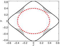
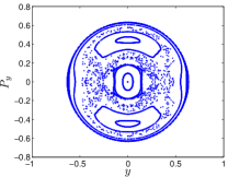
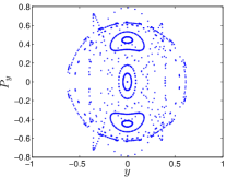
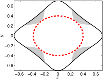
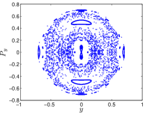
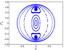
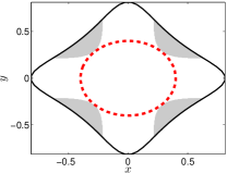
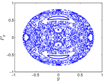
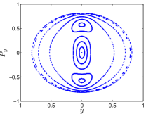
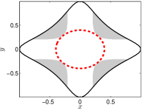
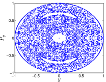
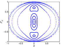
Figure 1: Effect of control on the model of Eq. (19). The first column shows the physical region (closed black curves) corresponding to the sequence of energies, $\frac{1}{5},\frac{1}{4},\frac{1}{3},\frac{1}{2}$ corresponding to $a,b,c,d$. The regions of negative eigenvalues (instability) are shown in gray. The second column shows the Poincaré plots for the uncontrolled system. The third column shows the Poincaré plots for the controlled system (Eq. (21) with $r=0.4$ for all cases). The (red) dashed line in column one shows the boundary of the control modification.

$(a_{I})$ $(a_{II})$ $(a_{III})$
$(b_{I})$ $(b_{II})$ $(b_{III})$
$(c_{I})$ $(c_{II})$ $(c_{III})$
$(d_{I})$ $(d_{II})$ $(d_{III})$
$(e_{I})$ $(e_{II})$ $(e_{III})$

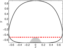
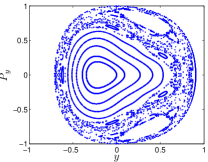
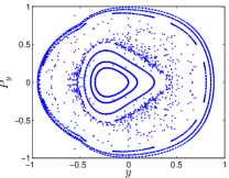
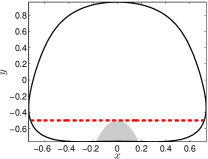
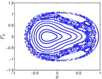
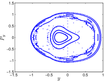
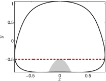
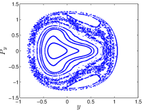
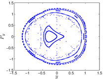
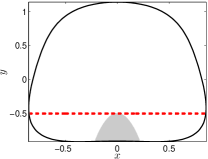
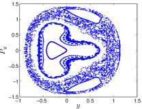
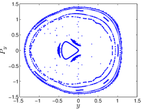
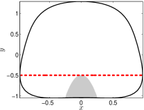
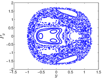
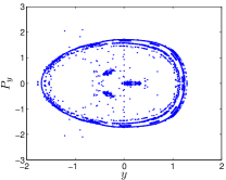
Figure 2: Effect of control on the model of Eq. (20). The first column shows the physical region (closed black curves) corresponding to the sequence of energies, $0.5,0.6,0.8,1.0,1.5$ corresponding to $a,b,c,d,e$. The regions of negative eigenvalues (instability) are shown in gray. The second column shows the Poincaré plots for the uncontrolled system. The third column shows the Poincaré plots for the controlled system (Eq. (22) with $\alpha=0.5$ for all cases). The (red) dashed line in column one shows the boundary of the control modification.

II Theory

It has been shown  appell ; BenZionPRL that a Hamiltonian system of the form (we use the summation convention)

$$H={{p^{i}}^{2}\over 2M}+V(x),$$ (1)

where $V$ is a function of space variables alone, can be put into the equivalent form

$$H_{G}={1\over 2M}g_{ij}p^{i}p^{j},$$ (2)

where $g_{ij}$ is conformal and is a function of the coordinates alone. One can easily see that the orbits described by the Hamilton equations for (2) coincide with the geodesics on a Riemannian space associated with the metric $g_{ij}$, i.e., it follows directly from the Hamilton equations associated with (1) that gutzwiller

$${\ddot{x}}_{\ell}=-\Gamma_{\ell}^{mn}{\dot{x}}_{m}{\dot{x}}_{n},$$ (3)

where the connection form $\Gamma_{\ell}^{mn}$ is given by

$$\Gamma_{\ell}^{mn}={1\over 2}g_{\ell k}\bigl{\{}{\partial g^{km}\over\partial x_{n}}+{\partial g^{kn}\over\partial x_{m}}-{\partial g^{nm}\over\partial x_{k}}\bigr{\}},$$ (4)

and $g^{ij}$ is the inverse of $g_{ij}$.

For a metric of conformal form

$$g_{ij}=\varphi\delta_{ij},$$ (5)

with inverse $g^{ij}=\varphi^{-1}\delta_{ij}$,on the hypersurface defined by $H_{G}=H=E=constant$, and assuming that the observable momenta are the same at every $t$, the requirement of equivalence implies that  BenZionPRL

$$\varphi={E\over E-V(x)}.$$ (6)

To see that the Hamilton equations obtained from (2) can, be put into correspondence with those obtained from the Hamiltonian of the potential model (1), we first note, from the Hamilton equations for (2), that

$${\dot{x}}_{i}={\partial H_{G}\over\partial p^{i}}={1\over M}g_{ij}p^{j}.$$ (7)

We then define the velocity field

$${\dot{x}}^{j}\equiv g^{ji}{\dot{x}}_{i}={1\over M}p^{j},$$ (8)

coinciding formally with one of the Hamilton equations implied by (1), for which we label the coordinates ${x^{j}}$.

To complete our correspondence with the dynamics induced by (1), consider the Hamilton equation for ${\dot{p}}^{i}$ generated by $H_{G}$,

$${\dot{p}}^{\ell}=-{\partial H_{G}\over\partial x_{\ell}}=-{1\over 2M}{\partial g_{ij}\over\partial x_{\ell}}p^{i}p^{j}.$$ (9)

With (8) this becomes

$${\ddot{x}}^{\ell}=-M^{\ell}_{mn}{\dot{x}}^{m}{\dot{x}}^{n},$$ (10)

where

$$M^{\ell}_{mn}\equiv{1\over 2}g^{\ell k}{\partial g_{nm}\over\partial x^{k}}.$$ (11)

Eq. (10) has the form of a geodesic equation, with a truncated connection form BenZionPRL . Note that performing parallel transport on the local flat tangent space of the Gutzwiller manifold (for which $\Gamma_{\ell}^{mn}$ and $g_{ij}$ are compatible), the resulting connection, after raising the tensor index to reach the Hamilton manifold, is exactly the “truncated” connection (11).

Substituting (5) and (6) into (10) and (11), the Kronecker deltas identify the indices of ${\dot{x}}^{m}$ and ${\dot{x}}^{n}$; the resulting square of the velocity cancels a factor of $(E-V)^{-1}$, leaving the Hamilton-Newton law derived from the Hamilton equations directly from (1). Eq. (10) is therefore a geometrically covariant form of the Hamilton-Newton law, exhibiting what can be considered an underlying geometry of standard Hamiltonian motion.

Since the coefficients $M^{\ell}_{mn}$ constitute a connection form, they can be used to construct a covariant derivative. It is this covariant derivative which must be used to compute the rate of transport of the geodesic deviation $\xi^{\ell}=x^{\prime\ell}-x^{\ell}$ along the (approximately common) motion of neighboring orbits in the Hamilton manifold, since it follows the geometrical structure of the geodesic curves on $\{x^{\ell}\}$.

The relation

$${\ddot{\xi}}^{\ell}=-2M^{\ell}_{mn}{\dot{x}}^{m}{\dot{\xi}}^{n}-{\partial M^{\ell}_{mn}\over\partial x^{q}}{\dot{x}}^{m}{\dot{x}}^{n}\xi^{q},$$ (12)

obtained from (10), can be factorized in terms of the covariant derivative

$$\xi^{\ell}_{;n}={\partial\xi^{\ell}\over\partial x^{n}}+M^{\ell}_{nm}\xi^{m}.$$ (13)

One obtains

$${{D_{M}}^{2}\over{D_{M}}t^{2}}\xi^{\ell}={{R_{M}}^{\ell}}_{qmn}{\dot{x}}^{q}{\dot{x}}^{n}\xi^{m},$$ (14)

where the index $M$ refers to the connection (11), and

$${{{R_{M}}^{\ell}}_{qmn}={\partial M^{\ell}_{qm}\over\partial x^{n}}-{\partial M^{\ell}_{qn}\over\partial x^{m}}+M^{k}_{qm}M^{\ell}_{nk}-M^{k}_{qn}M^{\ell}_{mk}}$$ (15)

corresponds to the curvature associated with the connection form $M^{\ell}_{mn}$ This expression does not coincide with the curvature of the Gutzwiller manifold (given by this formula with $\Gamma_{qm}^{\ell}$ in place of $M_{qm}^{\ell}$), but is a dynamical curvature which is appropriate for geodesic motion in $\{x^{\ell}\}$

With the conformal metric in noncovariant form (5),(6) (in the coordinate system in which (6) is defined), the dynamical curvature (15) can be written in terms of derivatives of the potential $V$, and the geodesic deviation equation (14) becomes

$${D^{2}{\bf\xi}\over Dt^{2}}=-{\cal V}P{\bf\xi},$$ (16)

where the matrix ${\cal V}$ is given by

$${\cal V}_{\ell i}=\bigl{\{}{3\over M^{2}v^{2}}{\partial V\over\partial x^{\ell}}{\partial V\over\partial x^{i}}+{1\over M}{\partial^{2}V\over\partial x^{\ell}\partial x^{i}}\bigr{\}}.$$ (17)

and

$$P^{ij}=\delta^{ij}-{v^{i}v^{j}\over v^{2}},$$ (18)

with $v^{i}\equiv{\dot{x}}^{i}$, defining a projection into a direction orthogonal to $v^{i}$.

Instability should occur if at least one of the eigenvalues of $P{\cal V}P$ is negative, in terms of the second covariant derivatives of the transverse component of the geodesic deviation. This condition is easily seen to be equivalent to the same condition imposed on the spectrum of ${\cal V}$, and is thus independent of the direction of the motion on the orbit.

The condition implied by the geodesic deviation equation (16), in terms of covariant derivatives, in which the orbits are viewed geometrically as geodesic motion, is a new condition for instability  BenZionPRL , based on the underlying geometry, for a Hamiltonian system of the form (1), providing new insight into the structure of the unstable and chaotic behavior of Hamiltonian dynamical systems. The method has been successfully applied to many potential models BenZionPRL ; BenZionPRE1 ; BenZionPRE2 ; yahalom . We now apply the method, which is simple and straightforward, since the instability criterion is defined locally in coordinate space, to extract from a chaotic Hamiltonian the part of the dynamics in the regions for which ${\cal V}$ has negative eigenvalues which lead to unstable motion . We show by direct simulation that this procedure is remarkably effective.

The results confirm the notion of the locality of our criterion, since the (local) removal of parts of the Hamiltonian inducing instability by this criterion strongly affects the global stability of the motion.

III Results and discussion

In the following we give some examples of Hamiltonian motion which are unstable and exhibit chaotic behavior. In two dimensions, the terms in the potential that break rotational symmetry have a form, in these examples, that induces chaotic behavior. The matrix ${\cal V}$ computed over the physically accessible region exhibits certain regions with negative eigenvalues. We have arranged our simulation to replace the Hamiltonian in the regions of negative eigenvalues by a Hamiltonian in which the symmetry breaking terms are either removed or for which the coupling coefficient is decreased, but in regions of positive eigenvalues, the Hamiltonian remains in its original form. The changes are carried in relatively small regions of the configuration space in the neighborhood of the regions of negative eigenvalues.

We take for illustration here a simple and important case of coupled harmonic oscillators with perturbation

$$V(x,y)=\frac{1}{2}(x^{2}+y^{2})+6x^{2}y^{2}$$ (19)

and a generalization of the Toda potential

$$V(x,y)=\frac{1}{2}(x^{2}+y^{2})+x^{2}y-\frac{1}{3}y^{3}+\frac{3}{2}x^{4}+\frac{1}{2}y^{4}.$$ (20)

The first of these is known to generate chaotic behavior; as we have shown previously, the transition to chaotic behavior as a function of energy and of the coupling to the perturbation is well described by our geometric criterion BenZionPRL . In the present work, we set the coupling to the chaos inducing perturbation to zero in the regions for which the geometric criterion results in negative eigenvalues.

In our previous study of the second example Eq. (20) we studied the sensitivity of the dynamical behavior to the choice of energy BenZionPRE2 . In the present work, at the energies for which the system exhibits chaotic behavior we have removed the chaos inducing perturbation in the regions for which the geometric criterion results in negative eigenvalues.

Fig. 1 shows the effects on the dynamical behavior of the change of the coupling to a stable value in the regions of negative eigenvalues for the perturbed oscillator potential (19). The results for different values of energy are shown; these values correspond to different sizes of the physically accessible region. Note that the radius of the region of positive eigenvalues does not change in this example.

The first row shows the physical region and the location of negative eigenvalues. The interior of the circle corresponds to a region in which no negative eigenvalue occur, chosen in this way to simplify the computation. The second row shows the surface of section Poincaré plot(surface of section) of the original uncontrolled Hamiltonian indicating chaotic dynamics. The third row shows the Poincaré plot generated by the controlled potential:

$$V(x,y)=\left\{\begin{matrix}\frac{1}{2}(x^{2}+y^{2})+6x^{2}y^{2}&x^{2}+y^{2}<r^{2}\\ \frac{1}{2}(x^{2}+y^{2})&x^{2}+y^{2}\geq r^{2}\end{matrix}\right.$$ (21)

where $r$ stands for the radius of the region of positive eigenvalues.

Fig. 2 shows the effect of control on second system (20), using the controlled potential:

$$V(x,y)=\left\{\begin{matrix}\frac{1}{2}(x^{2}+y^{2})+x^{2}y-\frac{1}{3}y^{3}+\frac{3}{2}x^{4}+\frac{1}{2}y^{4}&y>-\alpha\\ \frac{1}{2}(x^{2}+y^{2})&y\leq-\alpha\end{matrix}\right.$$ (22)

where $\alpha$ stands for the limit (a horizontal dashed line) of the region of positive eigenvalues.

In both cases, for sufficiently high energies the uncontrolled systems become less stable and a chaotic signature appears. We examine the method for different values of the energy, all corresponding to chaotic motion of the uncontrolled system. One can easily see that the Poincaré plots in controlled systems present almost completely regular motion.

IV Conclusion

We see from these computations that in regions of positive eigenvalues the Hamiltonian with chaos inducing terms do not generate instability. If the chaos inducing terms are removed or decreased in coupling in the regions of negative eigenvalues, the chaotic motion of the system is reduced or disappears. We conclude that the chaotic behavior of the system is associated with local properties of the Hamiltonian, and that our local criterion is effective in identifying these regions. Furthermore, our procedure provides an effective method for control of chaotic systems of this type.

References

- (1) E. Ott, C. Grebogi, and J. A. Yorke, Phys. Rev. Lett. 64, 1196 (1990).
- (2) T. Kapitaniak, Controlling Chaos (Academic Press, London, 1996).
- (3) U. Dressler and G. Nitsche, Phys. Rev. Lett. 68, 1 (1992).
- (4) K. Pyragas, Physics Letters A 170, 421 (1992).
- (5) W. L. Ditto, S. N. Rauseo, and M. L. Spano, Phys. Rev. Lett. 65, 3211 (1990).
- (6) C. Chandre, G. Ciraolo, F. Doveil, R. Lima, A. Macor, and M. Vittot, Phys. Rev. Lett. 94, 074101 (2005).
- (7) M. Vittot, M. Pettini, P. Ghendrih, G. Ciraolo, C. Chandre, and R. Lima, EPL (Europhysics Letters) 69, 879 (2005).
- (8) C. Chandre, G. Ciraolo, R. Lima, and M. Vittot, Journal of Physics Conference Series 7, 48 (2005).
- (9) Y. Zhang, S. Chen, and Y. Yao, Phys. Rev. E 62, 2135 (2000).
- (10) J. H. E. Cartwright, M. O. Magnasco, and O. Piro, Phys. Rev. E 65, 045203(R) (2002).
- (11) G. Ciraolo, F. Briolle, C. Chandre, E. Floriani, R. Lima, M. Vittot, M. Pettini, C. Figarella, and P. Ghendrih, Phys. Rev. E 69, 056213 (2004).
- (12) C. W. Kulp and E. R. Tracy, Phys. Rev. E 72, 036213 (2005).
- (13) Y. L. Bolotin, V. Y. Gonchar, A. A. Krokhin, P. H. Hernández-Tejeda, A. Tur, and V. V. Yanovsky, Phys. Rev. E 64, 026218 (2001).
- (14) M. Ding, W. Yang, V. In, W. L. Ditto, M. L. Spano, and B. Gluckman, Phys. Rev. E 53, 4334 (1996).
- (15) Y. Zhang, S. Chen, and Y. Yao, Phys. Rev. E 62, 2135 (2000).
- (16) Z. Wu, Z. Zhu, and C. Zhang, Phys. Rev. E 57, 366 (1998).
- (17) Y. Ben Zion and L. Horwitz, Phys. Rev. E 76, 046220 (2007).
- (18) L. Casetti, C. Clementi, and M. Pettini, Phys. Rev. E 54, 5969 (1996).
- (19) P. Cipriani and M. Di Bari, Phys. Rev. Lett. 81, 5532 (1998).
- (20) T. Kawabe, Phys. Rev. E 71, 017201 (2005).
- (21) M. Szydlowski and A. Krawiec, Phys. Rev. D 53, 6893 (1996).
- (22) M. Szydlowski and J. Szczesny, Phys. Rev. D 50, 819 (1994).
- (23) M. Szydlowski and A. Krawiec, Phys. Rev. D 47, 5323 (1993).
- (24) M. Szydlowski and A. Lapeta, Physics Letters A 148, 239 (1990).
- (25) L. Horwitz, Y. B. Zion, M. Lewkowicz, M. Schiffer, and J. Levitan, Phys. Rev. Lett. 98, 234301 (2007).
- (26) L. Casetti, M. Pettini, and E. G. D. Cohen, Physics Reports 337, 237 (2000).
- (27) Y. Ben Zion and L. Horwitz, Phys. Rev. E 78, 036209 (2008).
- (28) C. G. J. Jacobi, Vorlesungen über Dynamik (Verlag Reimer, Berlin, 1884).
- (29) J. Hadamard, J. Math. Pures et Appl. 4, 27 (1898).
- (30) A. Oloumi and D. Teychenné, Phys. Rev. E 60, R6279 (1999).
- (31) M. Gutzwiller, Chaos in Classical and Quantum Mechanics (Springer-Verlag, New York, 1990).
- (32) W. Curtis and F. Miller, Differentiable Manifolds and Theoretical Physics (Academic Press, New York, 1985).
- (33) J. Moser and E. Zehnder, Notes on Dynamical Systems (Amer. Math. Soc., Providence, 2005).
- (34) L. Eisenhardt, A Treatise on the Differential Geometry of Curves and Surfaces (Ginn and Company, Boston, 1909).
- (35) V. Arnold, Mathematical Methods of Classical Mechanics (Springer-Verlag, New York, 1978).
- (36) P. Appell, Dynamique des Systemes Mecanique Analytique (Gauthier-Villars, Paris, 1953).
- (37) H. Cartan, Calcul Differential et Formes Differentielle (Herman, Paris, 1967).
- (38) L. Landau and E. Lifshitz, Mechanics (Mir, Moscow, 1969).
- (39) D. Zerzion, L. Horwitz, and R. Arshansky, Jour. Math. Phys. 32, 1788 (1991).
- (40) A. Yahalom, J. Levitan, M. Lewkowicz, and L. Horwitz, submitted (unpublished).