Crystal and electronic structure of the room temperature organometallic ferrimagnet V(TCNE)₂. Analysis of numerical DoS and magnetic properties as related to orbital and spin-Hamiltonian models.

Abstract

We present a detailed analysis of the results of our numerical study of the crystal and electronic structure of the room temperature organometallic ferrimagnet of general composition V(TCNE)_x with $x\approx 2$. The results of the LSDA+$U$ study show that the experimentally determined structure complies with the magnetic measurements and thus can serve as a prototype structure for the entire family of the M(TCNE)₂ organometallic magnets. The results of the numerical study and of the magnetic experiments are interpreted using model Hamiltonians proposed here. This allowed us to obtain estimates of the critical temperature in three- and two-dimensional regimes and to give an explanation of the differences in behavior of probably isostructural V(TCNE)₂ and Fe(TCNE)₂ species.

1 Introduction

The most spectacular room temperature organometallic magnet of composition V(TCNE)${}_{x}\cdot y{\rm solvent}$ (where TCNE – 1 – stands for tetracyanoethylene – a well known organic electron acceptor; $x\approx 2$ and $y$ depends on the type of the solvent)

1

2

3

4

attracts a lot of attention since the time it had been synthesized yet in the beginning of the 1990’s [1]. It is an amorphous moisture sensitive precipitate with the outstanding critical temperature of the transition to the magnetically ordered state estimated to be of ca. 400 K. It is higher than the decomposition temperature (ca. 350 K ) which singles it out among its numerous analogs with a variety of involved organic acceptors (Ref. [2] – tetracyanopyrazine – 2; Ref. [3] – 7,7,8,8-tetracyano-p-quinodimethane – 3; Ref. [4] – tetracyanobenzene – 4) and of the metals (Ref. [5] – iron), synthesized in the following years, since none of them manifested as fascinating magnetic properties as the very first V(TCNE)₂ compound (see Table 1 [6]).

Generally one has to say that not only the critical temperature, but also other properties of the compounds of the considered class are sensitive to the details of the preparation procedure and/or the solvent employed. For example, the V-TCNE compound is known in two forms. The original of Ref. [1] coming from the reaction of V(C₆H₆)₂ with TCNE in the CH₂Cl₂ solution or obtained from V(CO)₆ with use of the CVD technique exhibits the saturation magnetization at the zero temperature which corresponds to approximately one unpaired electron per formula unit and in fact is somewhat lower than this value. However in Ref. [7] (see also a review [6]) a V(TCNE)₂ compound was reported containing tetrahydrofurane as a solvent with the saturation magnetization almost twice as strong compared to that of the original compound. For that reason hereinafter we shall refer to these two forms of the V(TCNE)₂ compound as the highly magnetic (HM) and the low magnetic(LM) ones.

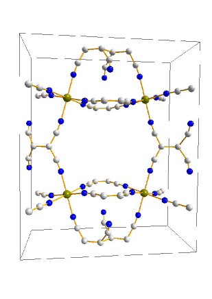
Figure 1: Structure of Fe(TCNE)₂ as coming from the synchrotron radiation study [8]. Each unit cell contains four formula units. The solvent molecules are omitted for clarity.

For more than one decade the amorphousity of the compound of interest did not allow anyone to make whatever definitive conclusion concerning its structure. The critical breakthrough became possible with the recent work [8] where the authors were able to establish the structure of the Fe²⁺ analog (presented in Fig. 1) of the V(TCNE)₂ compound using Rietveld refinement of the synchrotron powder diffraction data and to reveal its most remarkable features: the presence of the dimer form of the TCNE${}^{\dot{-}}$ radical-anion: $\left[\text{TCNE}\right]_{2}^{2-}\$= C₄(CN)${}_{8}^{2-}$ playing an important role in shaping the loose three-dimensional structure and assuring as well the three-dimensional character of magnetic interactions in the system.

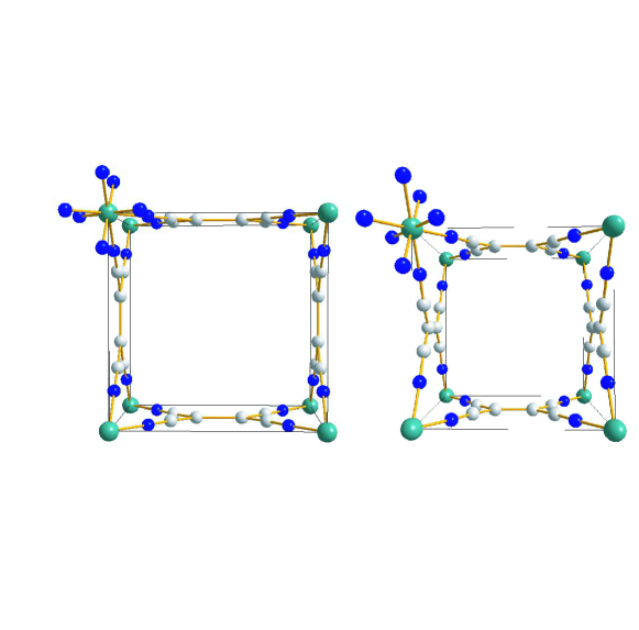
Figure 2: Hypothetical structures of V(TCNE)₂ following [9] (left) and following [10] (right).

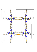
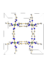
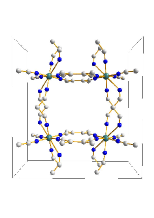
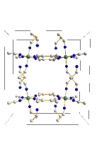
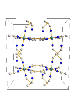
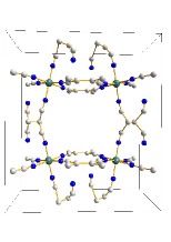
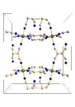
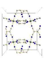
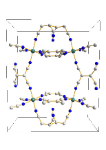
Figure 3: Schematic representation of the intermediate structures between the quadrupled ”principal” (left upper corner) and the experimental (right lower corner) ones.

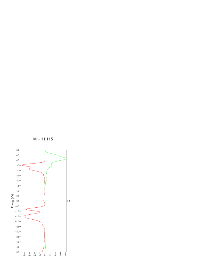
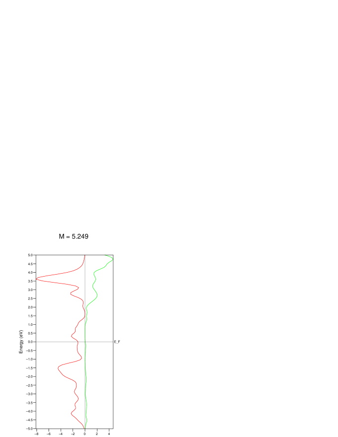
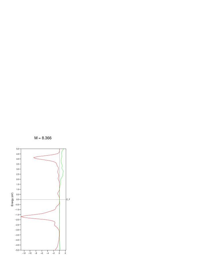
Figure 4: V-Densities of states in two spin channels for the limiting and an intermediate structures between the quadrupled ”principal” (left) and the experimental (right) ones. Observe different scale of the abscissa for different pictures. The magnetization in units of number of unpaired electrons per unit cell is indicated on top of each picture.

In our previous paper Ref. [10] we were able to demonstrate that the experimental structure represented in Fig. 1 can be easily related with one represented in Fig. 2a proposed yet in Ref. [9] in order to conform with the magnetic data on the V-TCNE compound available that time. That latter represented a simple cubic lattice with the vertices occupied by the vanadium ions. Two $ab$-faces of each cube remain empty whereas four others are filled by the TCNE units forming channels extended in the $c$-direction. In the structure presented in Fig. 2a the C=C bonds of the TCNE units are located in the same plane (as well perpendicular to the $c$-axis of the lattice) so that they are orthogonal to each other. It is not the unique possibility. An alternative structure differing from that of Fig. 2a by rotating the TCNE units placed in the $bc$-faces by 90^∘ in their respective planes is also possible. The result of such a rotation is presented in Fig. 2b. In this structure the central C=C bonds of the TCNE units are as previously orthogonal, but now they lay in orthogonal planes so that the axes of these bonds do not intersect rather cross each other. This structure has been called the ”principal” structure in Ref. [10]. The principal structure Fig. 2b can be easily put in the relation with the experimental one. If in the quadrupled unit cell $2a,2b,c$ of the principal structure four TCNE units extended in the $b$-direction are allowed to pairwisely rotate towards each other so that single C–C bonds can form between respective ethylenic carbon atoms thus yielding the [TCNE]${}_{2}^{2-}$=C₄(CN)${}_{8}^{2-}$ dimers and the V-TCNE sheets originally laying in the $ac$-planes are accordingly ruffled one finally arrives to the experimental structure of Fe(TCNE)₂ (Fig. 1). Intermediate structures along this hypothetical reaction path are presented in Fig. 3. For this sequence of structures we performed in Ref. [10] the LSDA + $U$ calculations with use of the VASP program suite Ref. [11] of the respective electronic structures and energies. Specifically, the PAW potential has been used and the values of the $U$ parameter for the V, N, and C atoms were respectively taken as 5.344, 4.840, and 4.428 eV. The calculations have been performed as follows: first the principal structure with the equalized lattice parameters have been quadrupled. This structure has been connected with the experimental structure by a straight line in the configuration space. Further details of the numerical treatment can be found in Ref. [10]. Its results are reproduced in Fig. 4.

The overall densities of states in two spin channels as given in Fig. 4 are obviously difficult to understand. One can only see some spin polarization of the upper filled bands as well as an evolution of a noticeable density of states near the Fermi level present in both spin channels in the initial state to the final state where the expected spin-polarized structure can be recognized which does not show any DoS in either of the spin channels at the Fermi level. In this paper we present a detailed analysis of the results of our numerical studies Ref. [10] of the models of V-TCNE room temperature organometallic ferrimagnet and expressed them in terms of the effective spin-Hamiltonian for a selection of interacting atomic/molecular states. The proposed model is then applied to analysis of a wider collection of experimental data available for this fascinating object and its Fe analog.

2 Detailed analysis of DoS

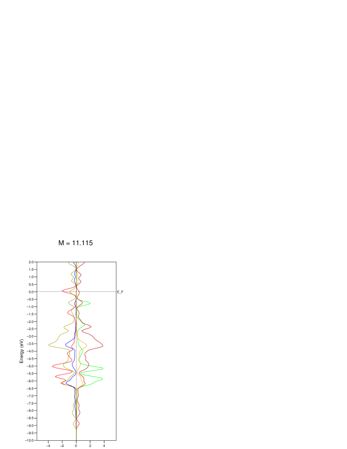
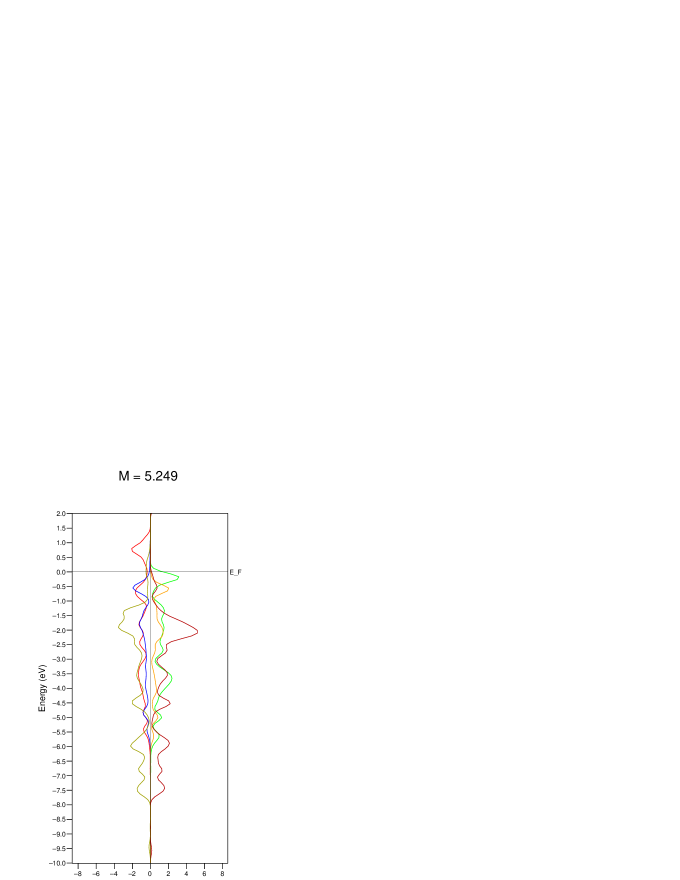
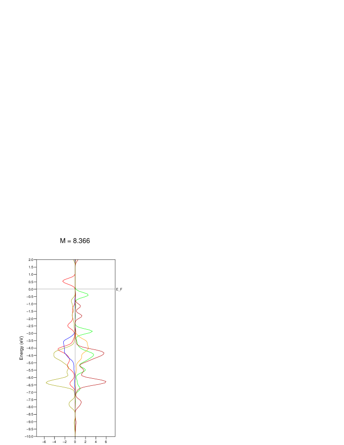
Figure 5: N-Densities of states in two spin channels for the limiting and an intermediate structures between the quadrupled ”principal” (left) and the experimental (right) ones. Red/green is the DoS of the N atoms in the V-TCNE layers, blue/yellow is that of the ”to be dangling” ones; olive green/dark red is that of those involved in the V-V bonding through the [TCNE]${}_{2}^{2-}$ units. Observe different scale of the abscissa for different pictures. The magnetization in units of number of unpaired electrons per unit cell is indicated on top of each picture.

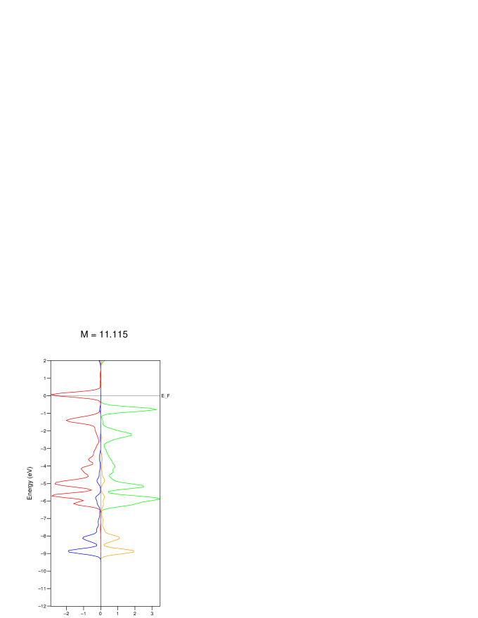
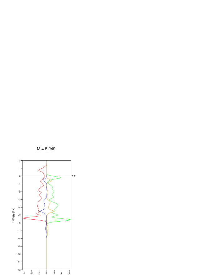
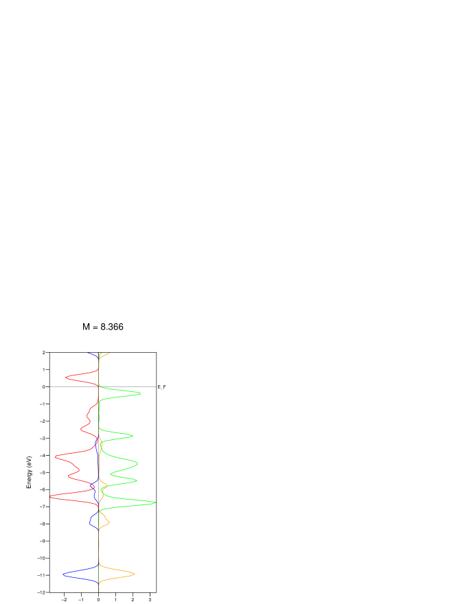
Figure 6: C-Densities of states in two spin channels for the limiting and an intermediate structures between the quadrupled ”principal” (left) and the experimental (right) ones. Red/green is the DoS of the C atoms in the V-TCNE layers, blue/yellow is that of those forming the C-C bonds in the [TCNE]${}_{2}^{2-}$ units. Observe different scale of the abscissa for different pictures. The magnetization in units of number of unpaired electrons per unit cell is indicated on top of each picture.

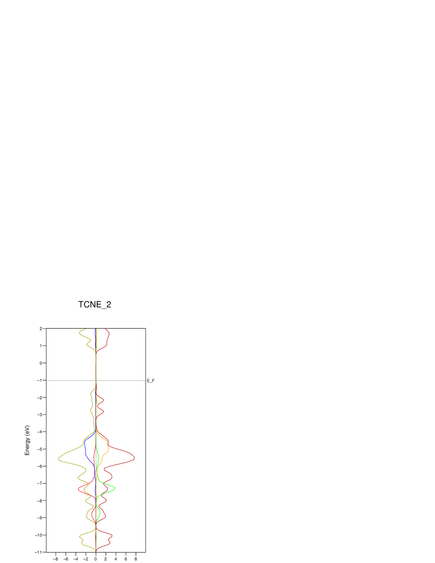
Figure 7: The projection of the DoS in two spin channels to the [TCNE]${}_{2}^{2-}$ units. in the ”experimental” structure [8]. Red/green is the DoS of the N atoms bonding the V-TCNE layers; blue/yellow is that of the ”dangling” ones; olive green/dark red is that of the C atoms.

In order to analyse the details of the evolution of the DoS features along the path going from quadrupled principal structure to the experimental one we performed a detailed study of projections of the DoS. In the initial structure the three bands in the $-9\div-11$ eV range are predominantly C-bands. Other bands are the well hybridized C-N-bands except the ”spin-left” band right below the Fermi level, which is predominantly contributed by the vanadium states. As one can see from Fig. 6 these are the $d$-states of vanadium atoms. Some vanadium stemming DoS in the range $-8\div-10$ eV are the $s$- and $p$-states of vanadium involved in the bonding with the nitrogen atoms. This can be seen on the corresponding N-projection of DoS in Fig. 7 from which one can deduce that the $s$- and $p$-states of vanadium hybridize predominantly with the N-states coming from the V-TCNE layers (see below). In order to deepen our understanding of the DoS presented in Fig. 5 we notice that even in that complex system the atoms involved are relatively easily classified into types. One can distinguish transition metal ions whose $d$-density is expected to contribute significantly to the spin polarized bands, the nitrogen atoms where one can expect significant DoS changes due to expected break of the pairs of excessive V-N bonds while going from the quadrupled principal structure to the experimental one. Analogously along the same route one can expect remarkable variations in the projection of the DoS to the carbon atoms forming the C-C bonds in the [TCNE]${}_{2}^{2-}$ units and to the carbon and nitrogen atoms in the ruffled V-TCNE layers. Other features of the DoS, however, are not expected to significantly vary along the path. Considering the evolution of the above-mentioned projections of the DoS along the path Fig. 3 as represented in Figs. 4 - 6 one can see the expected reconstruction of the projected DoS’s. For example, almost nothing happens to the $d$-bands along this path. They remain rigid triply degenerate ones and do not change their position relative to the Fermi level despite the fact that the coordination number of vanadium ions changes from eight in the quadrupled principal structure to six in the experimental one. This agrees with the numerical result concerning the distribution of spin polarization in the direct space: for all structures depicted in Fig. 3 the magnetic moments residing in the $d$-shells of vanadium ions range from 2.615 for the first (quadrupled principal) structure to 2.582 for the last (experimental) one i.e. are almost constant. The significant variation of the total magnetic moment along the ”reaction path” observed in our numerical experiment is to be almost completely attributed to that of the magnetic moments residing in the ”organic” part of the organometallic magnet. This is precisely what one should expect within the general picture including the formation of the [TCNE]${}_{2}^{2-}$ dimers. On the other hand the stability of the $d$-bands along the path can be only understood if one assumes that the break of two V-N bonds at each atom is at least partially compensated by shortening (strengthening) of other two bonds extended in the $b$-direction.

By contrast the projections of DoS to the characteristic organogenic atoms significantly modify along the  ”reaction path”. For example, the dominant part of the N-DoS is concentrated in two broad bands at ca. $-5$ and ca. $-6\div-6.5$ eV. The lower of the two is almost equally contributed by the nitrogen atoms of all three types and its position is stable throughout the path. The same applies to somewhat smaller contribution from the bonding N-atoms extended in the $b$-direction to this band. Their contribution to the upper of the two mentioned bands is noticeably spin-polarized. The density from the N atoms bearing the dangling lone pairs fairly manifests itself in the same band. Weak features in the N-DoS can be observed in the 4 eV wide range right below the Fermi level. The peak right below the Fermi level in the ”right-spin” channel in the initial structure is equally contributed by the ”bonding”, ”to be dangling”, and ”magnetic” nitrogens. (In general the DoS projections for the ”bonding” and ”to be dangling” nitrogens coincide in the initial structure). In the final structure this peak splits so that its upper part (”right-spin” channel right below the Fermi level) is contributed by the ”magnetic” nitrogens, whereas two peaks next to it in the bottom direction is contributed by the ”bonding” nitrogens. The contribution from the ”dangling” nitrogens contributes to the upper part of the wide band at ca. $-3.5\div-5.5$ eV.

Of particular interest is the evolution of the C-projection of the DoS. That on the ethylenic carbon atoms is most interesting. The ethylenic carbons can be further subdivided in two categories: those in the planes extended in the $a$ and $c$ horizontal directions and those extended in the vertical ($b$) direction and further involved in the rotation yielding the [TCNE]${}_{2}^{2-}$ units. At the initial stage both projected DoS are significantly polarized and both noticeably contribute to the ”right-spin” density right below the Fermi level (the DoS projection to the to be bonding atoms is not seen in the leftmost graph of Fig. 6 since at this point they are degenerate with the ”magnetic” projection and are masked by these latter). From further graphs of the DoS projected to the atoms forming the emerging C-C bonds one can conclude that such bonds represented in our study by two spin sub-bands for the left and right spin channels completely develop at a pretty late stage of the hypothetical transition: in the middle of the path the corresponding peaks in the density projections can be yet clearly seen in both spin channels near to the spin-polarized DoS of the ”magnetic” atoms, although the peaks corresponding to the emerging bonds are not polarized. By contrast the projection of DoS on the magnetic C-atoms in the horizontal planes develop two sub bands right above and below the Fermi level of which the lower one (right-spin) is completely occupied by electrons with the spin projection opposite to that of the electrons occupying the $d$-subband. This is in the fair agreement with the assumption concerning the nature of the subbands located in the vicinity of the Fermi level made in our previous paper Ref. [10].

3 Model Hamiltonians for V-TCNE system

3.1 Model Orbital Hamiltonian

Fascinating properties of the V(TCNE)₂ magnet call not only for numerical modelling, but also for some qualitative picture. However, for the final (”experimental”) structure all the DoS projections manifest themselves as very narrow bands. This indirectly indicates that the band picture used throughout the calculations is not completely adequate and that an adequate model must be given in terms of an effective Hamiltonian representing the electronic structure of the HM V(TCNE)₂ magnet (in its ”experimental” structure) in terms of some objects local in the direct space e.g. local spins similar to that proposed yet in Ref. [9]. As in the case of band models the most important one-electron states to be included are these contributing to the energy bands in the vicinity of the Fermi level. Based on our analysis of projected DoS performed in the previous Section we can conclude that the states of the [TCNE]${}_{2}^{2-}$ units contribute to the bands far away from the Fermi level. The DoS related to this unit goes away from the Fermi level along the ”reaction path”. Thus the observed electronic structure is primary one of the individual (ruffled) V-TCNE layer extended in the $ac$-plane. For constructing the Hamiltonian for this layer one can employ the unit cell of the principal model dropping from it the TCNE unit extended in the $b$-direction (and finally engaged in formation of the [TCNE]${}_{2}^{2-}$= C₄(CN)${}_{8}^{2-}$ dimers). According to Ref. [9] on the vanadium sites it suffice to consider only the $d$-shells of the metal ions which is also confirmed by our current analysis. The overlap of the $d$-shell of the metal ions with the $\sigma$-orbitals of the TCNE’s (including those implied in the model) ensures the standard two-over-three splitting of the $d$-shell characteristic for the octahedral environment. In the case of vanadium three unpaired electrons in the $d$-shell occupy respectively three orbitals in the $t_{2g}$-manifold. The basis orbitals $d_{xy}$, $d_{xz}$, and $d_{yz}$ can be characterized by the normal to the plane in which each of the orbitals lays – $\zeta$, $\eta$, and $\xi$ – are subsequently used in the notation. For the donor sites in the ruffled planes the $b_{3g}\left(\pi^{\ast}\right)$ LUMOs of the TCNE (singly occupied in the radical anion) are included. In each such a layer each metal ion is surrounded (coordinated) by four TCNE units which are in their turn coordinated to (surrounded by) four metal atoms. In this case the layer unit cell composition V:TCNE is 1:1.

The model Hamiltonian for the V(TCNE)₂ magnet, formulating the above ideas, has the general form:

$$H=\sum_{{\bf r}}\left(H_{d}({\bf r})+H_{a}({\bf r})+H_{da}({\bf r})+H_{dd}({\bf r})\right)$$ (1)

The contributions to it are the following. Operator $H_{a}({\bf r})$ describes electrons in the acceptor orbital of the TCNE${}^{\dot{-}}$ radical-anion in the ${\bf r}$-th unit cell:

$$\begin{array}[]{rcl}H_{a}({\bf r})&=&-\alpha_{a}\hat{n}_{a{\bf r}}+U_{aa}\hat{n}_{a{\bf r}\downarrow}\hat{n}_{a{\bf r}\uparrow}\\ \hat{n}_{a{\bf r}\sigma}&=&a_{{\bf r}\sigma}^{+}a_{{\bf r}\sigma};\hat{n}_{a{\bf r}}=\sum_{\sigma}\hat{n}_{a{\bf r}\sigma}\end{array}$$ (2)

Symbol $a_{{\bf r}\sigma}^{+}(a_{{\bf r}\sigma})$ is the operator creating (annihilating) an electron with the spin projection $\sigma$ on the acceptor orbital of the TCNE molecules in the ${\bf r}$-th unit cell. In eq. (2) the first term is the energy of attraction of an electron to the core of TCNE – the orbital energy of the $b_{3g}\left(\pi^{\ast}\right)$ LUMO shifted by the electrostatic field induced by the entire crystal environment. The second term in eq. (2) is the Hubbard one, effectively describing the Coulomb repulsion of electrons with opposite spin projections eventually occupying the same acceptor orbital.

The operator $H_{d}({\bf r})$ describes electrons in the $t_{2g}$-subshell of the $d$-shell of the vanadium ion in the ${\bf r}$-th unit cell:

$$H_{d}({\bf r}) = \left[-\alpha_{d}(\hat{n}_{\zeta{\bf r}}+\hat{n}_{\eta{\bf r}}+\hat{n}_{\xi{\bf r}})\right.+$$

$$+\left.(U_{dd}+2J_{dd})(\hat{n}_{\zeta{\bf r}\downarrow}\hat{n}_{\zeta{\bf r}\uparrow}+\hat{n}_{\eta{\bf r}\downarrow}\hat{n}_{\eta{\bf r}\uparrow}+\hat{n}_{\xi{\bf r}\downarrow}\hat{n}_{\xi{\bf r}\uparrow})\right]+$$

$$+\frac{(U_{dd}+J_{dd}/2)}{2}\sum_{\sigma,\sigma^{\prime}}(\hat{n}_{\zeta{\bf r}\sigma}\hat{n}_{\xi{\bf r}\sigma{\bf{}^{\prime}}}+\hat{n}_{\zeta{\bf r}\sigma}\hat{n}_{\eta{\bf r}\sigma{\bf{}^{\prime}}}+\hat{n}_{\xi{\bf r}\sigma}\hat{n}_{\eta{\bf r}\sigma{\bf{}^{\prime}}})+$$

$$-4J_{dd}(\hat{S}_{\zeta{\bf r}}\hat{S}_{\xi{\bf r}}+\hat{S}_{\zeta{\bf r}}\hat{S}_{\eta{\bf r}}+\hat{S}_{\xi{\bf r}}\hat{S}_{\eta{\bf r}})$$

$$\hat{n}_{\gamma{\bf r}\sigma} = \gamma_{{\bf r}\sigma}^{+}\gamma_{{\bf r}\sigma},\ \hat{n}_{\gamma{\bf r}}=\sum_{\sigma}\hat{n}_{\gamma{\bf r}\sigma};\gamma=\xi,\ \eta,\zeta.$$

In eq. (3.1) $\hat{n}_{\gamma{\bf r}\sigma}$ are the operators of the number of electrons with the spin projection $\sigma$ on the $d_{xy},d_{yz},$ and $d_{xz}$ orbitals of the vanadium ion in the ${\bf r}$-th unit cell. The spin operators and spin-operator product terms are defined by the well-known relations:

$$\hat{S}_{\gamma{\bf r}}\hat{S}_{\gamma^{\prime}{\bf r}} = 1/2(\hat{S}_{\gamma{\bf r}}^{+}\hat{S}_{\gamma^{\prime}{\bf r}}^{-}+\hat{S}_{\gamma^{\prime}{\bf r}}^{+}\hat{S}_{\gamma{\bf r}}^{-})+\hat{S}_{\gamma{\bf r}}^{z}\hat{S}_{\gamma^{\prime}{\bf r}}^{z}$$

$$\hat{S}_{\gamma{\bf r}}^{+} = \gamma_{{\bf r}\uparrow}^{+}\gamma_{{\bf r}\downarrow},\hat{S}_{\gamma{\bf r}}^{-}=\gamma_{{\bf r}\downarrow}^{+}\gamma_{{\bf r}\uparrow},\hat{S}_{\gamma{\bf r}}^{z}=1/2(\hat{n}_{\gamma{\bf r}\uparrow}-\hat{n}_{\gamma{\bf r}\downarrow}).$$

where the symbols $\gamma_{{\bf r}\sigma}^{+}\ (\gamma_{{\bf r}\sigma})$ represent the operators creating (annihilating) an electron with the spin projection $\sigma$ on the $d_{xy},d_{yz},$ and $d_{xz}$ orbitals of the vanadium ion in the ${\bf r}$-th unit cell.

The first row in the above operator describes the attraction of electrons in the $d$-orbitals to the cores of vanadium ions (shifted by the electrostatic field of the rest of the crystal). Two further rows describe the spin-symmetric part of the Coulomb interaction of electrons in the $d$-shell. The last row describes the spin dependent part of the Coulomb interaction of electrons in the $d$-shell (exchange). It is ultimately responsible for the Hund’s rule in atoms and for the high spin of the ground state of electrons in the $d$-shell. The contributions to the Hamiltonian eq. (1) described so far model isolated local states important for the crystal description. The magnetic order can only be possible due to various interaction terms. Operator $H_{da}({\bf r})$ describes the electron hopping between the $d$-states of vanadium ions and the acceptor states. The $d_{xy}$-state represented by the $\zeta_{{\bf r}\sigma}^{+}\ (\zeta_{{\bf r}\sigma})$ operators being of the (approximate) $\sigma$-symmetry with respect to the $ac$ plane (the ruffling of the V-TCNE plane is neglected) has no overlap with the LUMO’s of TCNE’s which are (again approximately) of the $\pi$-symmetry with respect to the same plane. Two others ($d_{xz}$- and $d_{yz}$-states represented respectively by the $\eta_{{\bf r}\sigma}^{+}\ (\eta_{{\bf r}\sigma})$ and $\xi_{{\bf r}\sigma}^{+}\ (\xi_{{\bf r}\sigma})$ operators) overlap with the LUMOs of two (different) neighbor TCNE units each. The phase relations between the orbitals involved in the model lead to such a distribution of signs at the one-electron hopping parameters that the hopping operator acquires the form:

$$H_{da}({\bf r})=-t_{da}\sum_{\sigma}{}\left[\xi_{{\bf r}\sigma}^{+}\left(a_{{\bf r}\sigma}+a_{{\bf r}+{\bf a}+{\bf c}\sigma}\right)-\eta_{{\bf r}\sigma}^{+}\left(a_{{\bf r}+{\bf a}\sigma}+a_{{\bf r}+{\bf c}\sigma}\right)\right]+h.c.$$ (4)

where the parameter $t_{da}>0$ describes the magnitude of the hopping between the acceptor state and the neighbor $d$-state.

The sum of the above contributions to the effective Hamiltonian in fact form that for an isolated V-TCNE layer. In the ”experimental” structure the diamagnetic C₄(CN)${}_{8}^{2-}$ units seem to effectively isolate the V(TCNE) sheets from each other. Nevertheless, one should assume that certain indirect interaction between the $d$-states in the $b$-direction is possible through the mediation of the [TCNE]${}_{2}^{2-}$ units. It was proposed in Ref. [10] to use an effective hopping similar to eq. (4). Since it is any way an effective interaction it can be chosen in a way which fits better to the method the system is treated. For this reason we postpone the discussion of this term.

In our previous paper Ref. [10] we considered the band model of the V-TCNE organometallic magnet as derived from the orbital Hamiltonian eqs. (1) - (4) and employed them for analysis of results of our numerical experiments performed with use of the VASP package. These latter are, however, in a kind of fundamental contradiction with the physics of the system at hand. This manifests itself in the very narrow bands coming out of calculation, as we already mentioned. The reason is that the hopping parameter $t_{da}$ entering eq. (4) which are generally responsible for extension of one-electron states over the crystal (band formation) and which are proportional to the overlap between the orbitals represent the smallest energy scale in the system. Generally it leads to a break of the delocalized (band) picture and makes a local description to be more adequate. The latter can be sequentially derived by treating perturbatively the hopping operator eq. (4). It yields the effective Hamiltonian of the Heisenberg form in terms of the spins of electrons occupying the local states (orbitals) involved. Its parameters are estimated in Appendix A.

The overall result comes out as a spin Hamiltonian of the form:

$$\begin{array}[]{ccc}H_{{\rm spin}}^{{\rm layer}}&=&-4J_{dd}\sum\limits_{{\bf r}}(\hat{S}_{\zeta{\bf r}}\hat{S}_{\xi{\bf r}}+\hat{S}_{\zeta{\bf r}}\hat{S}_{\eta{\bf r}}+\hat{S}_{\xi{\bf r}}\hat{S}_{\eta{\bf r}})+\\ &&+2K_{da}\sum\limits_{{\bf r}}\left[\hat{S}_{\xi{\bf r}}\left(\hat{S}_{a{\bf r}}+\hat{S}_{a{\bf r}+{\bf a}+{\bf c}}\right)+\hat{S}_{\eta{\bf r}}\left(\hat{S}_{a{\bf r}+{\bf a}}+\hat{S}_{a{\bf r}+{\bf c}}\right)\right]\end{array}$$ (5)

which describes effective magnetic interactions in an isolated layer. It must be complemented by interlayer interactions. If the vanadium ions in adjacent layers are coupled by an an effective hopping an analogous perturbative procedure results in the antiferromagnetic sign of the effective magnetic interaction. This contradicts to the existence of the nonzero overall magnetization in the V-TCNE magnets below the critical temperature (with the antiferromagnetic interlayer coupling the magnetization of one layer would be cancelled by that of another). For that reason we have to supplement the Hamiltonian eq. (5) by an effective interlayer interaction with the ferromagnetic sign of the corresponding exchange parameter. It cannot directly come from any perturbative treatment of the hopping. By contrast some mechanism of ferromagnetic coupling described e.g. in Refs. [12] or [13] and implemented in papers [14, 15] devoted to the exchange in metallocene based organometallic magnets (Miller-Epstein magnets) acting through the [TCNE]${}_{2}^{2-}$ units might be expected. Indeed as one can see from the Fig. 7 despite the fact the the states located in the [TCNE]${}_{2}^{2-}$ units are pulled up and down from the vicinity of the Fermi level, some spin polarization of these bands particularly of those which are contributed by the ”bonding” nitrogens indicates the involvement of the [TCNE]${}_{2}^{2-}$ units in transfer of magnetic interactions between the $d$-shells in the $b$-direction (between the layers).

With this caveat the spin Hamiltonian written in terms of ”true” electronic spins is the following:

$$\begin{array}[]{ccc}H_{{\rm spin}}&=&-4J_{dd}\sum\limits_{{\bf r}}(\hat{S}_{\zeta{\bf r}}\hat{S}_{\xi{\bf r}}+\hat{S}_{\zeta{\bf r}}\hat{S}_{\eta{\bf r}}+\hat{S}_{\xi{\bf r}}\hat{S}_{\eta{\bf r}})+\\ &+&2K_{da}\sum\limits_{{\bf r}}\left[\hat{S}_{\xi{\bf r}}\left(\hat{S}_{a{\bf r}}+\hat{S}_{a{\bf r}+{\bf a}+{\bf c}}\right)+\hat{S}_{\eta{\bf r}}\left(\hat{S}_{a{\bf r}+{\bf a}}+\hat{S}_{a{\bf r}+{\bf c}}\right)\right]\\ &+&2K_{dd}\sum\limits_{{\bf r}}\left(\hat{S}_{\xi{\bf r}}+\hat{S}_{\eta{\bf r}}+\hat{S}_{\zeta{\bf r}}\right)\left(\hat{S}_{\xi{\bf r+b}}+\hat{S}_{\eta{\bf r+b}}+\hat{S}_{\zeta{\bf r+b}}\right)\end{array}$$ (6)

The Hamiltonian eq. (6) is not a standard Heisenberg Hamiltonian usually used to describe magnetic properties of insulators. This latter is written in terms of the effective local spins residing at each atomic magnetic center. In our case the vanadium ions represetn such nontrivial magnetic centers bearing effective spins in the $d$-shells:

$$\hat{S}_{d{\bf r}}=\sum_{\gamma}\hat{S}_{\gamma{\bf r}}.$$ (7)

According to Ref. [16] using the effective spins is, however, an approximation since the transition from the representation of the effective Hamiltonian in terms of the of individual electronic spins-$\frac{1}{2}$ eq. (6) which can be sequentially derived from the model orbital Hamiltonian eqs. (1) - (4) by perturbative treatment of the hopping term eq. (4) to the phenomenological Hamiltonian eq. (8) operating with the effective spins eq. (7) is only possible if the exchange interactions of all individual spins in one magnetic center (in our case – the V ion) with those in the other magnetic center (in our case the effective spin in TCNE${}^{\dot{-}}$ coincides with the individual one) are equal. This is obviously not the case since the electronic spin $\hat{S}_{\zeta{\bf r}}$ in the $d$-shell to the first approximation does not interact with the spin residing in any of acceptor orbitals.

This generally poses the problem since in the Hamiltonian eq. (6) at least the exchange parameters $J_{dd}$ and $K_{da}$ can be independently determined respectively by eq. (18) and atomic spectra, whereas the parameter $J_{\bot}$ in eq. (8) remains completely empirical quantity. The fact that $J_{dd}\gg K_{da}$ in eq. (6) allows to approximately replace the spins of separate electrons in the ${\bf r}$-th $d$-shell by the operator of the total spin of the respective $d$-shell. Further details of this transition are given in Appendix B.

The phenomenological Hamiltonian written in terms of the effective spins eq. (7) to be used for modeling the entire crystal is:

$$\begin{array}[]{ccc}H_{{\rm phen}}&=&J_{\|}\sum\limits_{{\bf r}}\hat{S}_{d{\bf r}}\left[\hat{S}_{a{\bf r}}+\hat{S}_{a{\bf r}+{\bf a}}+\hat{S}_{a{\bf r}+{\bf c}}+\hat{S}_{a{\bf r}+{\bf a}+{\bf c}}\right]+\\ &&+J_{\bot}\sum\limits_{{\bf r}}\hat{S}_{d{\bf r}}\hat{S}_{d{\bf r}+{\bf b}}\end{array}$$ (8)

In the next Section we apply it to analysis of magnetic properties of the HM V(TCNE)₂ material.

4 Magnetic properties of V(TCNE)₂ as interpreted with use of phenomenological Hamiltonian

The magnetic and thermodynamic properties of the HM V(TCNE)₂ material must be derived from the phenomenological Hamiltonian eq. (8). Two types of data will be of interest for us: the critical temperature of transition into magnetically ordered state and the temperature dependence of spontaneous magnetization. The mean field estimates of the critical temperature used so far in the literature lack the account of structural information. It is important to realize that the quantities of interest are sensitive to these details as represented in the respective Hamiltonians.

The commonly used (see e.g. Ref. [6]) symmetric mean field formula:

$$\theta_{N}^{MF}=\frac{zJ_{eff}}{3}S_{d}\left(S_{d}+1\right)$$

(where $T=\theta/k_{B}$) ignores the acceptor spins and sets $z$ to be the number of indirectly neighboring magnetic metal ions. It yields the quadratic dependence of the critical temperature on the spin of the metal ion. On the other hand according to Ref. [8] the critical temperature for the magnetically ordered state of a material with two types of spins ($S_{d}$ and $S_{a}(=1/2)$) is described by the mean field formula:

$$\theta^{\rm MF}_{N}=\frac{\left|J^{\rm MF}_{{\rm eff}}\right|}{3}\sqrt{Z_{ad}Z_{da}}\sqrt{S_{d}(S_{d}+1)S_{a}(S_{a}+1)}$$

(The factor of two is dropped here to get the formula to conform with the Hamiltonian definition accepted in the present paper). This formula appears as a zero interlayer coupling limit of the mean field expression for the Néel temperature in a ferrimagnet eq. (41) derived in Appendix C. In Ref. [8] it had been applied to the Fe(TCNE)₂ compound for which the structure measurements have been performed there. It, however, brings up two complications – one theoretical and another experimental. From the experimental point of view we notice that the above formula as well as formula eq. (41) is effectively linear in $S_{d}$ rather than quadratic (in the high anisotropy limit). For that reason even the mean field estimates of the exchange parameters as given in Table 1 must be reconsidered since the latter had been obtained with use of the quadratic dependence. As one can see from the structure the choice of $Z_{ad}=Z_{da}=4$ yields the estimate of the mean field exchange parameter for the Fe(TCNE)₂ compound of $J^{\rm MF}_{{\rm eff}}({\rm Fe})=$ 43 K and for the V(TCNE)₂ compound – $J^{\rm MF}_{{\rm eff}}({\rm V})=183$ K. Both values are significantly larger than those given in Table 1, but it is remarkable that the difference between them (to be explained) reduces from the factor of larger than five to that of 4.25. We notice that following the assumption of Ref. [24] and using $Z_{dd}=6$ for the V(TCNE)₂ compound further reduces the difference and the value of the exchange parameter for the latter, but from our point of view it cannot be substantiated within the scope of the model considered in the present paper.

From the theoretical point of view, even the improved molecular field expression eq. (41) has that disadvantage that it predicts a nonvanishing ordering temperature for $J_{\perp}=0$. It is obviously wrong and such an estimate is not acceptable in the context where a strong anisotropy might be expected on the structure basis. As it has been mentioned the model must be complemented by the interlayer interactions between the effective spins $3/2$ on the vanadium sites mediated by the diamagnetic (closed shell) [TCNE]^2- units. Remarkably enough the sign of this interaction must be ferromagnetic (the magnetic moments residing in the layers must be pointing in the same direction) to ensure the existence of the net spontaneous magnetization in the three-dimensional sample, although in general one has to expect antiferromagnetic sign of such an interaction [12] (see below).

In a presumably rather anisotropic situation brought by tentative difference in mechanisms of the intralayer and interlayer interactions (respectively ”antiferromagnetic kinetic exchange” for the intralayer interaction and the ”ferromagnetic superexchange” for the interlayer one) the critical temperature has to be estimated from the spin-wave treatment taking an adequate care about the anisotropy of the effective spin-spin interaction and at least providing a correct asymptotic value of the critical temperature for the vanishing interlayer coupling $J_{\perp}$. This is done by the formula

$$M_{s}=M_{0}\left[1-\left(\frac{\theta}{\theta_{\mathrm{N}}}\right)^{\frac{3}{2}}\right]$$ (9)

expressing the Bloch $T^{\frac{3}{2}}$ law for the temperature dependence of the spontaneous magnetization as derived in Appendix D with the critical (Néel) temperature given by:

$$\theta_{\mathrm{N}}=\frac{4\pi}{\zeta^{\frac{2}{3}}(\frac{3}{2})}\frac{1}{S_{d}-S_{a}}\sqrt[3]{\left(S_{d}+S_{a}\right)^{2}S_{d}^{4}S_{a}^{2}}\left[J_{\parallel}^{2}\left|J_{\perp}\right|\right]^{\frac{1}{3}}$$ (10)

– the 3D structure-specific relation of the effective exchange interaction to the Néel temperature.

The assumptions used in Appendix D for deriving the formula eq. (10) are not satisfied in strongly anisotropic systems where $\left|J_{\perp}\right|\ll J_{\parallel}$. In this limit the Néel temperature is to be determind from the transcendental equation:

$$\frac{1}{4\pi}\frac{S_{d}-S_{a}}{S_{d}S_{a}}\frac{\theta_{\mathrm{N}}}{J_{\|}}\frac{1}{S_{d}+S_{a}}\log\left(\frac{S_{d}-S_{a}}{S_{d}^{2}}\frac{\theta_{\mathrm{N}}}{\left|J_{\bot}\right|}\right)=1,$$ (11)

and the magnetization is given by:

$$M_{s}=M_{0}\left[1-\frac{1}{4\pi}\frac{S_{d}-S_{a}}{S_{d}S_{a}}\frac{1}{S_{d}+S_{a}}\frac{\theta}{J_{\|}}\log\left(\frac{S_{d}-S_{a}}{S_{d}^{2}}\frac{\theta}{\left|J_{\bot}\right|}\right)\right]$$ (12)

provided $\theta$ is close enough to $\theta_{\mathrm{N}}$.

Neither three-dimensional (3D) or two-dimensional (2D) estimates of the Néel temperature eqs. (10) and (11), respectively, permits to determine the longitudinal and transversal interactions independently and to establish by this the amount of anisotropy. The effective exchange interaction $J^{\rm SW}_{\rm eff}=\sqrt[3]{J_{\parallel}^{2}J_{\perp}}$ as derived from eq. (10) and the experimental Néel temperature for the HM V(TCNE)₂ compound amounts $J^{\rm SW}_{\rm eff}({\rm V})=$ 36 K. This is due rather large numerical value of the transition coefficient in eq. (10) coupling the effective exchange interaction with the Néel temperature (11.376 for the structure depicted in Fig. 1 and $S_{d}=\frac{3}{2};S_{a}=\frac{1}{2}$). This result is in a general agreement with the result of Ref. [18] which yields the corresponding coefficient to be 9.937 for a simple cubic ferrimagnet with the same values of the effective spins. (It is not clear how the estimate of ca. 100 K for $J^{\rm SW}_{\rm eff}({\rm V})$ is obtained in Ref. [23] since is also based on assumption of a simple cubic lattice magnetic structure, but apparently uses some different coefficient). It also stresses the different character of averaging of intralayer and interlayer exchange parameters in the mean field (arithmetic mean) and in the spin-wave (geometric mean) approximations. At the high anisotropies the geometric mean provides much stronger dependence of the effective exchange on the interlayer exchange than the arithmetic mean.

Whatever value of $J^{\rm SW}_{\rm eff}$ leaves a wide range of possibilities since each pair of values of $J_{\perp}$ and $J_{\parallel}$ yielding the above value of $J^{\rm SW}_{\rm eff}({\rm V})$ conforms with the experimental data on magnetization. It has to be realized, however, that using the Bloch $T^{\frac{3}{2}}$ law for the magnetization in the entire temperature range below $T_{N}$ is an extrapolation of the data obtained at low temperatures. In order to check its validity in a wider temperature range we notice that according to it the magnetization depletion at the an intermediate temperature (225 K) amounts the factor of 0.592 which looks out to be in an acceptable agreement with experiment which shows the magnetization depletion by a factor of ca. 0.6 at this temperature as compared to that at $T=0$.

In the HM V(TCNE)₂ case the measured magnetization values are available up to 300 K. The Bloch $T^{\frac{3}{2}}$-law for the temperature dependence of spontaneous magnetization results in a simple formula for the slope of the magnetization vs. temperature in the Néel point:

$$-\frac{3}{2}\frac{M_{0}}{T_{\rm N}}$$ (13)

As one can derive from the magnetization data on the HM compound given in Ref. [6] the slope of the magnetization of the HM material in the Néel point amounts $\displaystyle-1.4\frac{M_{0}}{T_{\rm N}}$ which is a fair extrapolation of the last measured points. It suggests the 3D regime for the HM material in the entire temperature interval up to the Néel point. Nevertheless the possibility of transition to the 2D regime at $T>300$ K cannot be a priori excluded. Then for the 2D regime the slope of magnetization vs. temperature in the Néel point is:

$$-M_{0}\frac{k_{B}}{4\pi J_{\parallel}}\frac{S_{d}-S_{a}}{S_{d}S_{a}}\frac{1}{S_{d}+S_{a}}\left(1+\log\left(\frac{S_{d}-S_{a}}{S_{d}^{2}}\frac{k_{B}T_{\rm N}}{\left|J_{\perp}\right|}\right)\right)$$ (14)

When combined with eq. (11) it yields:

$$-M_{0}\left(\frac{k_{B}}{4\pi J_{\parallel}}\frac{S_{d}-S_{a}}{S_{d}S_{a}}\frac{1}{S_{d}+S_{a}}+\frac{1}{T_{\rm N}}\right)$$ (15)

Employing the value of the slope extracted from Fig. 1 of Ref. [6] we derive $k_{B}T_{\rm N}=2.4\pi J_{\parallel}$, and inserting experimental (extrapolated) value of $T_{\rm N}$ yields immediately $J_{\parallel}=54$ K and together with the value of $J^{\rm SW}_{\rm eff}$ extracted from low temperature data allows to estimate anisotropy to be ($J_{\parallel}/J_{\perp}\approx 3$). At the above intermediate temperature (225 K) the 2D estimate with this anisotropy shows the depletion of magnetization to be 0.595 of the maximal value at 0 K as well in a perfect agreement with experiment, which shows that the available data on the temperature dependence of magnetization in HM V(TCNE)₂ do not allow to distinguish between the 3D and 2D regimes. It must be admitted that in general the above value of anisotropy is not large enough ($\sim 3$) for the 2D regime to install. This analysis, however, allows us to set bounds for the value $J_{\parallel}$ in the V(TCNE)₂ compound as derived from the spin-wave treatment: it appears that this compound resides in the 3D regime so that the above value of anisotropy must be considered as a maximal possible in this material. Otherwise even higher Néel temperatures (although not accessible expreimentally due to material’s decomposition) still conforming to the applicability conditions ($2J_{\perp}S_{d}^{2}\ll\theta\ll 4J_{\parallel}S_{d}S_{a}$) Ref. [25] of the logarithmic formula eq. (11) should have to be admitted.

Applying analogous treatment to the Fe(TCNE)₂ compound for which the structure presented in Fig. 1 is experimentally established yields the following: $J^{\rm SW}_{\rm eff}=9.5$ K (the coefficient of 12.914 coming from eq. (10) with $S_{d}=2$ is used). With the anisotropy of $2.5^{3}=15.625$ the 2D estimate of the Néel temperature is 124 K again in a fair agreement with the experiment. The value of $J_{\parallel}$ is then 24 K. This turns out to be not that much different from the upper boundary for the same quantity for the V(TCNE)₂ compound yielding the ratio of the intralayer exchange parameters for the two materials of maximum only two, instead of 4 $\div$ 5 stipulated by the mean field estimates, and only 1.5 if the isotropic regime is accepted for the V(TCNE)₂ compound.

This latter value can be fairly explained by addressing the formulae of Appendix A and the spectroscopic data. From eq. (18) it follows that the ratio $J_{\parallel}({\rm V})/J_{\parallel}({\rm Fe})$ of the intralayer parameters for the vanadium and iron compounds is that of the squared hopping parameters $t_{da}$. (We assume here that due to similarity of the environment in these two compounds the energy denominators in eq. (18) given by eq. (A) are the same for the both compounds since the values of ionisation potentials of the V²⁺ and Fe²⁺ ions which are respectively 29.55 and 30.90 eV as coming from Ref. [26] and similarly close estimates for the electron affinities for these ions). According to suggestion by [27] thoroughly tested numerically in Refs. [28, 29, 30] the amounts of the crystal field splitting in the coordination compounds are proportional to analogous expressions: squares of the hopping parameters divided by some (other) energy denominators, which are, however, also approximately equal in similar compounds. Thus the proportion holds:

$$\frac{J_{\parallel}({\rm V})}{J_{\parallel}({\rm Fe})}=\frac{10Dq({\rm V})}{10Dq({\rm Fe})}$$

for pairs of similar complexes in each side of the proportion. For the right side of the proportion we find with the values of Refs. [31, 32] $10Dq({\rm V})=14700$ cm^-1, $10Dq({\rm Fe})=10900$ cm^-1 to be 1.35 for the hexacoordinate octahedral complexes with acetonitile, which basically explains the above ratio 1.5 of the intralayer exchange parameters. Of course, the significant difference of anisotropies in these two materials remains to be understood.

This can be tentatively done with use of the Goodenough-Kanamori rules [12]. Indeed, the difference in the interlayer interactions requiring an explanation is too large, so that probably a qualitative distinction between the two materials is responsible for it. As we mentioned above the simplistic application of the Goodenough-Kanamori rules in the present situation yields an antiferromagnetic sign of the interlayer interaction (the situation falls into the Goodenough-Kanamori cation-anion-cation category in the 180^∘ geometry). Thus the observed ferromagnetic sign of the interlayer interaction appears as a result of ferromagnetic contributions of the higher order. Such contributions depend qualitatively on the possibility to take advantage of the intrashell ferromagnetic interactions which in their turn depend on the occupancies of the atomic orbitals in the d-shells of the interacting transition metal cations. (Importance of such terms in the context of organometallic magnets had been stressed in Refs. [14, 15]). It can be easily understood that the conditions for appearance of the compensating ferromagnetic terms are very much different for the V²⁺ and Fe²⁺ ions. Indeed, in the case of the V²⁺ ion two $d$-orbitals remain empty and can participate in the one-electron transfer coupled with the intrashell exchange eq.(21) compensating otherwise dominating antiferromagnetic kinetic exchange. In the case of the Fe²⁺ ion only one doubly occupied $d$-orbital can take part in a similar process, so that one can expect that the compensating contribution will be significantly weaker in the case of the Fe(TCNE)₂ compound eventually leading to much weaker overall ferromagnetic interlayer interaction, than in the case of the V(TCNE)₂ compound.

5 Discussion

In the present Section we apply the models proposed above to analysis of experimantal data available for the HM V(TCNE)₂ and Fe(TCNE)₂ compounds.

First of all we notice that the spin polarization per unit cell (number of electrons with spin up minus that with spin down) which can be related with observed magnetization per formula unit. We see that the calculation performed for V(TCNE)₂ at the experimental structure of Fe(TCNE)₂ depicted on Fig. 1 shows the spin polarization of ca. 8 spins-1/2 per unit cell corresponding to two netto unpaired electrons per formula unit which is in a fair agreement with the magnetization measured in the HM V(TCNE)₂ compound. On the other hand the LM V(TCNE)₂ material manifests a weaker saturation magnetization, namely corresponding to ca. one netto unpaired electron per formula unit. This allows to think about certain differences in the structures of two materials. Nevertheless, both experimentally observed values (ca. 10$\cdot$10³ emu$\cdot$Oe$\cdot$mol^-1 and 6$\cdot$10³ emu$\cdot$Oe$\cdot$mol^-1, respectively) both deviate from the theoretical values of 11.2 and 5.6 giving the magnetization produced by the integer number of netto spin-polarized electrons in an assumption of the Landé factor being equal to 2.

When trying to extend the model Ref. [8] of the Fe(TCNE)₂ compound to analysis of the V(TCNE)₂ compound the authors Ref. [8] argued that the vanadium compound must have some structure different from the iron one since the saturation magnetization in it is lower and approximately corresponds to two spins $1/2$ compensating (interacting antiferromagnetically with) one spin $3/2$ per formula unit. From this observation the authors of Ref. [8] conclude that the interlayer interactions must be mediated by $\mu_{4}$-TCNE radical-anions, as it has been suggested yet in [9], rather by the [TCNE]${}_{2}^{2-}$ dimers. This argument applies of course only to the LM form of the V(TCNE)₂ material since for its HM form our numerical experiment shows that for the experimental structure of the Fe(TCNE)₂ compound the calculated magnetization fairly corresponds to the experimental value obtained on the HM V(TCNE)₂ material. Incidentally, the magnetization values obtained numerically at intermediate structures on the  ”reaction path” depicted on Fig. 3 allows us to assume that some similar structures obtained from structures of Fig. 2 by rotations of some TCNE units may present in the LM V-TCNE material. This view had found a recent support from the computational side in Ref. [33] where a structure for the LM form of V(TCNE)₂ has been proposed. It would be fair to say (although it is not said in Ref. [33]) that this structure as well descends from the structures of Refs. [9, 10]. Specifically, in order to obtain the structure of Ref. [33] one has to rotate the TCNE molecule laying in the $bc$-face of either of these structures depicted in Fig. 2 in each of the unit cells around the diagonal of the face (or around an axis going through the pair of trans-nitrogen atoms of that TCNE unit) by ca. 90^∘ so that two other N-atoms of each rotating TCNE unit go out of coordination with the V ions. Such a structure corresponds as that of Ref. [9] and the principal one (see above) of Ref. [10] to two TCNE${}^{\dot{-}}$ units per unit cell each bearing one unpaired electron and thus expectedly yield the overall magnetization corresponding to one unpaired electron per formula unit. For such a structure the magnetic interaction parameters obtained in Ref. [33] are almost isotropic ($J_{\perp}=720$ K and $J_{\parallel}=690$ K) which is also not surprising since the character of interactions between the V $d$-shells and LUMO’s of the TCNE${}^{\dot{-}}$ units are fairly the same in either direction. The numerical values of the exchange parameters obtained in Ref. [33] are for sure considerable overestimates of the true ones since the Néel temperature derived from them either by the mean field or spin-wave methods exceeds the experimental value by orders of magnitude. Nevertheless, applying the spin-wave theory similar to that described in Section D results in the estimate for $k_{B}T_{\rm N}=9.14J^{\rm SW}_{\rm eff}$ which yields the numerical value of $J^{\rm SW}_{\rm eff}$ for the LM form of V(TCNE)₂ material of 45 K in fair agreement with the similar above estimates for the intralayer effective exchange parameters. It must also be admitted that the spin-wave treatment of the model of Ref. [33] leaves the question of the reason of complete disagreement of the temperature dependence of the magnetization in the LM compound as given in Ref. [6] with the Bloch law which should be expected for almost isotropic ferrimagnet unanswered.

6 Conclusion

In the present paper we performed detailed analysis of our numerical results concerning thinkable structure of room-temperature organometallic magnet V(TCNE)₂ as manifested in the corresponding projections of DoS. Similar analysis of projected DoS for a sequence of structures leading to the tentative experimental structure of V(TCNE)₂ is performed as well. Model spin Hamiltonian is developed for analysis and interpretation of numerical results and experimental data. Analysis of magnetic data in terms of the approximate models derived from the phenomenological Hamiltonian is performed. A remarkable correspondence between experimental (structural and magnetic) data on V(TCNE)${}_{x}\cdot y\ {\rm solvent}$ and numerical model has been observed previously: magnetization corresponding to two unpaired electrons per formula unit in fair agreement with experiment on HM V-TCNE material derived from V(CO)₆ by CVD technique is obtained numerically for V(TCNE)₂ taken in the relaxed experimental Fe(TCNE)₂ geometry Ref. [10]. Now it is complemented by the detailed analysis of the magnon spectrum of this model. The possible transition between the low-temperature 3D and the high-temperature 2D regimes is discussed. Estimates of parameters of the proposed spin-Hamiltonian as treated in the spin-wave approximation are derived from the experimental data on the Néel temperature and the temperature dependence of magnetization. The differences in magnetic behavior of probably isostructural HM V(TCNE)₂ and Fe(TCNE)₂ are tentatively explained.

Appendix A Spin Hamiltonian as derived from orbital model Hamiltonian

Simple estimates of the parameters of the spin Hamiltonian eq, (6) can be based on considerations dating back to Ref. [12] as specified for the current situation. For the idealized geometry of M(TCNE)₂ compounds where the M-TCNE layers are assumed to be planar the one-electron hopping parameters $t_{da}$ are those between the $b_{3g}\left(\pi^{\ast}\right)$ singly occupied orbital of the TCNE${}^{\dot{-}}$ radial-anion and one of the $d$-orbitals of the $\pi$-symmetry with respect to the abovementioned plane ($d_{xz}$ and $d_{yz}$). For a pair of the TCNE${}^{\dot{-}}$ and V²⁺ ions described by the Hamiltonians, eqs. (2) and (3.1), respectively, the energy of the bare ground state reads:

$$E_{0}=-\alpha_{a}-3\alpha_{d}+3U_{dd}-21/4J_{dd}$$ (16)

and does not depend on the way the spins in these sites are coupled. The one-electron hopping couples them with two states with one electron transferred between the two sites (from one of the $d$-states to the $a$-state and from the $a$-state to one of the $d$-states). The energies of the charge transfer states are respectively:

$$E_{d\rightarrow a} = -2\alpha_{a}-2\alpha_{d}+U_{aa}+U_{dd}-3J_{dd}/2$$

$$E_{a\rightarrow d} = -4\alpha_{d}+6U_{dd}+29/4J_{dd}$$

They both correspond to the lower spin of the state of the two ions which results, as usual, to a Heisenberg-type interaction of two 1/2 electron spins:

$$2K_{da}\hat{S}_{\gamma{\bf r}}\hat{S}_{a{\bf r}}$$ (17)

occupying the overlapping orbitals (here $\gamma$ refers to that of the three $d$-orbitals which overlaps with the particular $a$-orbital) with the effective exchange constant given by:

$$K_{da}=t_{da}^{2}(\Delta E_{d\rightarrow a}^{-1}+\Delta E_{a\rightarrow d}^{-1})>0,$$ (18)

where

$$\Delta E_{d\rightarrow a} = \alpha_{d}-\alpha_{a}+U_{aa}-2U_{dd}+15/4J_{dd}=\Delta\alpha+U_{aa}-2U_{dd}+15/4J_{dd}>0,$$

$$\Delta E_{a\rightarrow d} = \alpha_{a}-\alpha_{d}+3U_{dd}+50/4J_{dd}=-\Delta\alpha+3U_{dd}+50/4J_{dd}>0,$$

$$\Delta\alpha = \alpha_{d}-\alpha_{a}>0;\Delta E_{a\rightarrow d}>\Delta E_{d\rightarrow a}.$$

On the other hand the charge transfer energies can be expressed through the spectral ionization potentials of the respective ions, their electron affinities and the energy shifts $C_{d}$ and $C_{a}$ of these quantities induced by the Coulomb field of the surrounding crystals already mentioned:

$$\Delta E_{d\rightarrow a} = I_{d}-A_{a}-g_{ad}>0,,$$

$$\Delta E_{a\rightarrow d} = I_{a}-A_{d}-g_{ad}>0,$$

$$I_{d} = I^{0}_{d}-C_{d}>0;I^{0}_{d}=\alpha^{0}_{d}-(n_{d}-1)U_{dd}$$ (19)

$$A^{0}_{d} = I^{0}_{d}-U_{dd}$$

$$I_{a} = \alpha^{0}_{a}-C_{a}>0.$$

(here we omitted the intraatomic exchange parameters $J_{dd}$ known to be by orders of magnitude smaller than other quantities relevant here and included the electron-hole interaction energies $g_{ad}$ previously absorbed in $\alpha$’s).

The interaction eq. (17) must be repeated for each interacting pair of electronic spins (pair of orbitals, coupled by the electron hopping operator). For the V ion in the crystal the terms appear for the $\xi$- and $\eta$-states on each atom.

For the pair of metal ions interacting through the [TCNE]${}_{2}^{2-}$ unit the one electron hopping is effectively possible not only between the states in the $t_{2g}$-manifolds of the ions involved, but also between other remaining $d$-orbitals. By this the states admixed to the spin degenerate bare gound state of the pair of ions may have either lower or higher spin which leads both to the antiferromagnetic contribution of the form:

$$\frac{4t_{dd}^{2}}{\Delta E_{d\rightarrow d}}$$ (20)

and of the ferromagnetic contribution of the form:

$$-\left(\frac{4t_{dd}^{\prime}}{\Delta E_{d\rightarrow d}}\right)^{2}J_{dd}$$ (21)

where the hopping parameters $t_{dd}$ and $t_{dd}^{\prime}$ have the same order of magnitude. The terms of the antiferromagnetic sign appear for each pair of the $d$-orbitals coupled by the hopping, whereas the terms of the ferromegnetic sign appear all singly occupied orbitals in both shells provided an empty or a doubly occupied in the given $d$-shell couples with a singly occupied orbital in other $d$-shell through the hopping.

Appendix B Phenomenological Hamiltonian for effective spins and its relation to the spin Hamiltonian

The phenomenological Hamiltonian written in terms of the effective spins eq. (7) to be used for modeling the entire crystal has the form of eq. (8)

In order to obtain it we follow the general recipes given in Ref. [16] for obtaining the spin-wave spectrum and write the general Heisenberg equations of motion for the spin-raising operators $\hat{S}_{d{\bf r}}^{+},\hat{S}_{a{\bf r}}^{+}$. They read:

$$\begin{array}[]{lll}i\hbar\frac{\partial}{\partial t}\hat{S}_{d{\bf r}}^{+}&=&-J_{\bot}\left(\hat{S}_{d{\bf r}}^{z}\hat{S}_{d{\bf r}\pm{\bf b}}^{+}-\hat{S}_{d{\bf r}}^{+}\hat{S}_{d{\bf r}\pm{\bf b}}^{z}\right)\\ &&+J_{\|}\left[\hat{S}_{d{\bf r}}^{z}\left(\hat{S}_{a{\bf r}}^{+}+\hat{S}_{a{\bf r}+{\bf a}+{\bf c}}^{+}+\hat{S}_{a{\bf r}+{\bf a}}^{+}+\hat{S}_{a{\bf r}+{\bf c}}^{+}\right)\right.\\ &&-\left.\hat{S}_{d{\bf r}}^{+}\left(\hat{S}_{a{\bf r}}^{z}+\hat{S}_{a{\bf r}+{\bf a}+{\bf c}}^{z}+\hat{S}_{a{\bf r}+{\bf a}}^{z}+\hat{S}_{a{\bf r}+{\bf c}}^{z}\right)\right]\\ i\hbar\frac{\partial}{\partial t}\hat{S}_{a{\bf r}}^{+}&=&J_{\|}\left[\hat{S}_{a{\bf r}}^{z}\left(\hat{S}_{d{\bf r}}^{+}+\hat{S}_{d{\bf r}-{\bf a}-{\bf c}}^{+}+\hat{S}_{d{\bf r}-{\bf a}}^{+}+\hat{S}_{d{\bf r}-{\bf c}}^{+}\right)\right.\\ &&-\left.\hat{S}_{a{\bf r}}^{+}\left(\hat{S}_{d{\bf r}}^{z}+\hat{S}_{d{\bf r}-{\bf a}-{\bf c}}^{z}+\hat{S}_{d{\bf r}-{\bf a}}^{z}+\hat{S}_{d{\bf r}-{\bf c}}^{z}\right)\right]\end{array}$$ (22)

In the spin-wave approximation the operators $\hat{S}_{d}^{z}$ and $\hat{S}_{a}^{z}$ are replaced by their average values in the magnetic (ordered) phase:

$$\hat{S}_{d{\bf r}}^{z}\rightarrow\left\langle\hat{S}_{d}^{z}\right\rangle=\frac{3}{2};\hat{S}_{a{\bf r}}^{z}\rightarrow\left\langle\hat{S}_{a}^{z}\right\rangle=-\frac{1}{2}$$ (23)

so that the equations of motion get the form:

$$\begin{array}[]{lll}i\hbar\frac{\partial}{\partial t}\hat{S}_{d{\bf r}}^{+}&=&-J_{\bot}\left(\frac{3}{2}\hat{S}_{d{\bf r}\pm{\bf b}}^{+}-3\hat{S}_{d{\bf r}}^{+}\right)\\ &&+J_{\|}\left[\frac{3}{2}\left(\hat{S}_{a{\bf r}}^{+}+\hat{S}_{a{\bf r}+{\bf a}+{\bf c}}^{+}+\hat{S}_{a{\bf r}+{\bf a}}^{+}+\hat{S}_{a{\bf r}+{\bf c}}^{+}\right)+2\hat{S}_{d{\bf r}}^{+}\right]\\ i\hbar\frac{\partial}{\partial t}\hat{S}_{a{\bf r}}^{+}&=&J_{\|}\left[-\frac{1}{2}\left(\hat{S}_{d{\bf r}}^{+}+\hat{S}_{d{\bf r}-{\bf a}-{\bf c}}^{+}+\hat{S}_{d{\bf r}-{\bf a}}^{+}+\hat{S}_{d{\bf r}-{\bf c}}^{+}\right)-6\hat{S}_{a{\bf r}}^{+}\right].\end{array}$$ (24)

Going to the Fourier transforms of the raising operators we get:

$$\begin{array}[]{lll}i\hbar\frac{\partial}{\partial t}\hat{S}_{d{\bf k}}^{+}&=&-3J_{\bot}\left(\cos k_{b}-1\right)\hat{S}_{d{\bf k}}^{+}+J_{\|}\left[\frac{3}{2}\Omega_{{\bf k}}\hat{S}_{a{\bf k}}^{+}+2\hat{S}_{d{\bf k}}^{+}\right]\\ i\hbar\frac{\partial}{\partial t}\hat{S}_{a{\bf k}}^{+}&=&-J_{\|}\left[\frac{\Omega_{{\bf k}}^{\ast}}{2}\hat{S}_{d{\bf k}}^{+}+2\hat{S}_{a{\bf r}}^{+}\right]\\ \Omega_{{\bf k}}&=&1+\exp(ik_{a})+\exp(ik_{c})+\exp(ik_{a}+ik_{c})\end{array}$$ (25)

which must be complemented by analogous system of equations for the spin lowering operators $\hat{S}_{d{\bf r}}^{-},\hat{S}_{a{\bf r}}^{-}$.

On the other hand the Heisenberg equations of motion for the operators $\hat{S}_{\zeta{\mathbf{r}}}^{+},\hat{S}_{\eta{\mathbf{r}}}^{+},\hat{S}_{\xi{\mathbf{r}}}^{+},$ and $\hat{S}_{a{\mathbf{r}}}^{+}$ as derived from eq. (6) (after the Fourier transformation is performed) form a system of four equations of motion for the Fourier components of the spin-$\frac{1}{2}$ raising operators for each wave vector ${\mathbf{k}}$. It can be rewritten with use of ${\mathbf{k}}$-dependent 4$\times$4 matrices acting on the vectors $\hat{S}_{{\mathbf{k}}}^{+}$ with the components $\hat{S}_{\zeta{\mathbf{k}}}^{+},\hat{S}_{\eta{\mathbf{k}}}^{+},\hat{S}_{\xi{\mathbf{k}}}^{+},\hat{S}_{a{\mathbf{k}}}^{+}$:

$$i\hbar\frac{\partial}{\partial t}\hat{S}_{{\mathbf{k}}}^{+}=M({\mathbf{k}})\hat{S}_{{\mathbf{k}}}^{+}$$ (26)

where

$$M({\mathbf{k}})=A+T({\mathbf{k}})+L({\mathbf{k}})$$ (27)

and the matrix

$$A=J_{dd}\left(\begin{array}[]{cccc}4&-2&-2&0\\ -2&4&-2&0\\ -2&-2&4&0\\ 0&0&0&0\end{array}\right)$$ (28)

describes the spin fluctuations in the $d$-shells, the matrix

$$T({\mathbf{k}})=K_{dd}\left(\cos{\mathbf{k}}_{b}\left(\begin{array}[]{cccc}1&1&1&0\\ 1&1&1&0\\ 1&1&1&0\\ 0&0&0&0\end{array}\right)-3\left(\begin{array}[]{cccc}1&0&0&0\\ 0&1&0&0\\ 0&0&1&0\\ 0&0&0&0\end{array}\right)\right)$$ (29)

describes the spin wave propagation in the $b$-direction (transversal to the V-TCNE) planes and the matrix

$$L({\mathbf{k}})=K_{da}\left(\begin{array}[]{cccc}0&0&0&0\\ 0&1&0&\frac{1}{2}Q_{c{\mathbf{k}}}\\ 0&0&1&\frac{1}{2}Q_{a{\mathbf{k}}}\\ 0&-\frac{1}{2}Q_{c{\mathbf{k}}}^{\ast}&-\frac{1}{2}Q_{a{\mathbf{k}}}^{\ast}&-2\end{array}\right)$$ (30)

with

$$\begin{array}[]{rcl}Q_{a{\mathbf{k}}}&=&1+e^{-ik_{a}-ik_{c}}\\ Q_{c{\mathbf{k}}}&=&e^{-ik_{a}}+e^{-ik_{c}}\end{array}$$ (31)

desribes the spin-wave propagation in the $ac$-plane i.e. in the individual V-TCNE layer. Going to the linear combitations of the spin fluctuation operators in the $d$-shell: $\hat{S}_{\zeta{\mathbf{k}}}^{+}+\hat{S}_{\eta{\mathbf{k}}}^{+}+\hat{S}_{\xi{\mathbf{k}}}^{+};\ -\hat{S}_{\zeta{\mathbf{k}}}^{+}+\hat{S}_{\eta{\mathbf{k}}}^{+};\ -\hat{S}_{\zeta{\mathbf{k}}}^{+}+\hat{S}_{\xi{\mathbf{k}}}^{+}$ introduces the fluctuation of the effective spin of the $d$-shell (the first combination) and incidentaly diagonalizes the sum of the first two matrix terms $A+T({\mathbf{k}})$ yielding the eigenvalues: $0;\ 3K_{dd}\left(\cos{\mathbf{k}}_{b}-1\right);\ 6J_{dd}-3K_{dd}>0$ of which the zero one refers to precession of the $\frac{1}{2}$ spin in the acceptor orbital, the next one refers to precession of the total spin of the $d$-shell, and the doubly degenerate highest eigenvalue corresponds to excitations changing the total spin of the $d$-shell. The interaction matrix $L({\mathbf{k}})$ in this basis acquires the form:

$$\frac{K_{da}}{6}\left(\begin{array}[]{llll}-12&Q_{c{\mathbf{k}}}^{*}-2Q_{a{\mathbf{k}}}^{*}&Q_{a{\mathbf{k}}}^{*}-2Q_{c{\mathbf{k}}}^{*}&-Q_{a{\mathbf{k}}}^{*}-Q_{c{\mathbf{k}}}^{*}\\ 3Q_{a{\mathbf{k}}}&4&-2&2\\ 3Q_{c{\mathbf{k}}}&-2&4&2\\ 3\left(Q_{a{\mathbf{k}}}+Q_{c{\mathbf{k}}}\right)&2&2&4\end{array}\right)$$ (36)

The states corresponding to the excitations of the $d$-shell (the above matrix is written so that they are the second and the third ones) are of much higher energy than the states corresponding to precession of the effective spins in two types of sites of the model. For that reason the former can be excluded. To do so we treat $L({\mathbf{k}})$ as a perturbation with the smallness parameter $\frac{K_{da}}{J_{dd}}$ and in the zero order we obtain an operator acting in the two-dimensional subspace spanned by the vector with the components $\hat{S}_{\zeta{\mathbf{k}}}^{+}+\hat{S}_{\eta{\mathbf{k}}}^{+}+\hat{S}_{\xi{\mathbf{k}}}^{+}=\hat{S}_{d{\mathbf{k}}}^{+};\ \hat{S}_{a{\mathbf{k}}}^{+}$:

$$\left(\begin{array}[]{ll}-2K_{da}&-\frac{1}{6}\left(Q_{a{\mathbf{k}}}^{*}+Q_{c{\mathbf{k}}}^{*}\right)K_{da}\\ \frac{1}{2}\left(Q_{a{\mathbf{k}}}+Q_{c{\mathbf{k}}}\right)K_{da}&\frac{2K_{da}}{3}-3K_{dd}\left(1-\cos k_{b})\right)\end{array}\right)$$ (37)

Comparing eq. (37) with eq. (25) and noticing that $\Omega_{k}=Q_{a{\mathbf{k}}}^{*}+Q_{c{\mathbf{k}}}^{*}$ we arrive to the conclusion that they coincide after setting $\left|S_{\xi}^{z}\right|=\left|S_{\eta}^{z}\right|=\frac{1}{2}=\frac{1}{3}\left|S_{d}^{z}\right|$ and $K_{dd}=-J_{\bot};K_{da}=3J_{\|}$ which establishes the required relation between the spin wave treatments of the Hamiltonians eq. (6) and eq. (8). The first order correction to eq. (37) has the form:

$$\frac{K_{da}^{2}}{9J_{dd}}\left(\begin{array}[]{ll}\frac{1}{2}(2-\cos k_{a}-\cos k_{c}+2\cos k_{c}\cos k_{a})&\frac{1}{12}\Omega_{k}^{*}\\ -\frac{1}{4}\Omega_{k}&\frac{1}{3}\end{array}\right),$$ (40)

but it is not used hereinafter.

Appendix C Mean Field treatment of the phenomenological Hamiltonian.

In order to obtain a structure dependent mean field estimate for the Néel temperature of the V-TCNE material we use the method described in Ref. [21]. Accordingly the Néel temperature for a system comprising two types of magnetic centers with effective spins $S_{d}$ and $S_{a}$ so that each center of the with spin $S_{d}$ has $Z_{dd}$ neighbours of the same type, $Z_{da}$ neighbours with the spin $S_{a}$ etc. with the interactions between the nearest neighbors of the specific type given by $J_{dd},J_{da}$ etc. satisfies the equation:

$$\left|\begin{array}[]{cc}J_{dd}Z_{dd}S_{d}\left(S_{d}+1\right)-3\theta_{N}^{MF}&J_{da}Z_{da}S_{d}\left(S_{d}+1\right)\\ J_{da}Z_{ad}S_{a}\left(S_{a}+1\right)&J_{aa}Z_{aa}S_{a}\left(S_{a}+1\right)-3\theta_{N}^{MF}\end{array}\right|=0$$

where we used the fact that $J_{ad}=J_{da}$. For the structure represented in Fig. 1 and modelled by the Hamiltonian eq. (8) we set $S_{a}=\frac{1}{2}$. Then $Z_{ad}=Z_{da}=4$; $Z_{dd}=2;Z_{aa}=0$ (acceptors do not have acceptor neighbors in this model). In the notation of eq. (8) $J_{dd}=J_{\perp};J_{da}=J_{\parallel}$, so that we obtain:

$$\theta_{N}^{MF}=\frac{2J_{\perp}}{3}S_{d}\left(S_{d}+1\right)+\sqrt{\frac{J_{\perp}^{2}}{9}S_{d}^{2}\left(S_{d}+1\right)^{2}+\frac{4}{3}J_{\parallel}^{2}S_{d}\left(S_{d}+1\right)}$$

which in the limit of strong anisotropy yields the following mean field estimate:

$$\theta_{N}^{MF}=\frac{2J_{\perp}}{3}S_{d}\left(S_{d}+1\right)+J_{\parallel}\sqrt{\frac{4}{3}S_{d}\left(S_{d}+1\right)}$$ (41)

which flows to the the limiting expression used in Ref. [8] for the single Fe-TCNE layer with the variance of the factor of two which results from the different definition of the Hamiltonian in Refs. [8, 21].

Appendix D Spin-wave model of magnetic properties of V(TCNE)₂

Now we address the spin-wave theory of the M(TCNE)₂ ferrimagnets described by the phenomenological Hamiltonian eq. (8) in order to derive its magnetic properties. The temperature dependence of magnetization and the Néel temperature (that at each the magnetization of each sublattice vanishes) are controlled by the spectrum of the lowest energy excitations: spin waves (magnons). Calculation of these properties is customary performed with use of the Holstein-Primakoff Ref. [17] representation of the magnons. This latter had been many times derived for the ferrimagnets with relatively simple crystal lattice Refs. [18, 19]. These derivations are based on the Green’s function techniques. The present case differs from those described there by a combination of the alternation of the interaction sign ($J_{\|}$ and $J_{\bot}$ have opposite signs) and a relatively complex form of the structure factors which makes the Green’s function too cumbersome and also prevents from using directly the the general formulae derived previously. We perform the required derivation for the present structure for certainty using the equation of motion method. It evolves as follows. Each term in the phenomenological Hamiltonian eq. (8) has the form:

$$J_{12}\hat{S}_{1}\hat{S}_{2}=J_{12}\left[\hat{S}_{1}^{z}\hat{S}_{2}^{z}+\frac{1}{2}\left(\hat{S}_{1}^{+}\hat{S}_{2}^{-}+\hat{S}_{1}^{-}\hat{S}_{2}^{+}\right)\right]$$ (42)

If the pair of the above spins couples ferromagnetically ($J_{12}<0$) the Holstein-Primakoff operators $b_{i}(b_{i}^{+})$ annihilating (crearing) an elementary excitation (magnon) at the i-th site are introduced by the relations:

$$\hat{S}_{i}^{+} = \sqrt{2S_{i}-\hat{n}_{i}}b_{i}$$

$$\hat{S}_{i}^{-} = b_{i}^{+}\sqrt{2S_{i}-\hat{n}_{i}}$$ (43)

$$\hat{S}_{i}^{z} = S_{i}-\hat{n}_{i};\hat{n}_{i}=b_{i}^{+}b_{i}$$

The operators $b_{i}(b_{i}^{+})$ so defined obey the boson commutation relations:

$$\left[b_{i}^{+},b_{i^{\prime}}^{+}\right]=\left[b_{i},b_{i^{\prime}}\right]=0;\left[b_{i}^{+},b_{i^{\prime}}\right]=\delta_{ii^{\prime}}$$ (44)

After being inserted in the above Hamiltonian term the square roots are expanded and the terms non higher of the second order in the boson operators $b_{i}$ are kept (linear spin-wave approximation) so that one gets:

$$J_{12}\hat{S}_{1}\hat{S}_{2}=J_{12}S_{1}S_{2}-J_{12}\left(S_{1}\hat{n}_{2}+\hat{n}_{1}S_{2}\right)+J_{12}\sqrt{S_{1}S_{2}}\left(b_{1}^{+}b_{2}+b_{2}^{+}b_{1}\right)$$ (45)

If the pair of effective spins couples antiferromagnetically ($J_{12}>0$) the Holstein-Primakoff bosons are obtained by a more complex trick which, first, requires a transformation of the spins residing on the $m$-th site in the unit cell by the rotation matrices $\omega_{m}$:

$$\tilde{S}_{i} = \hat{S}_{i}\omega_{i};\hat{S}_{i}=\omega_{i}^{\dagger}\tilde{S}_{i}$$ (46)

In the assumption of the common quantization axis for all spins in the crystallographic unit cell one can select the rotations as follows:

$$\omega_{1}=\begin{pmatrix}1&0&0\\ 0&1&0\\ 0&0&1\end{pmatrix};\omega_{2}=\begin{pmatrix}1&0&0\\ 0&-1&0\\ 0&0&-1\end{pmatrix}$$ (47)

in the basis of the coordinate spin components $x,y,z$ or

$$\omega_{1}=\begin{pmatrix}1&0&0\\ 0&1&0\\ 0&0&1\end{pmatrix};\omega_{2}=\begin{pmatrix}0&1&0\\ 1&0&0\\ 0&0&-1\end{pmatrix}$$ (48)

in the basis of the tensor spin components $+,-,z$. Then the interaction term rewrites:

$$J_{12}\hat{S}_{1}\hat{S}_{2}=-J_{12}\hat{S}_{1}^{z}\tilde{S}_{2}^{z}+\frac{1}{2}J_{12}\left(\hat{S}_{1}^{+}\tilde{S}_{2}^{+}+\hat{S}_{1}^{-}\tilde{S}_{2}^{-}\right)$$ (49)

The boson operators for the transformed spins are then defined by the same relations as the nontransformed ones which yields the following interaction term:

$$J_{12}\hat{S}_{1}\hat{S}_{2}=-J_{12}S_{1}S_{2}+J_{12}\left(S_{1}\hat{n}_{2}+\hat{n}_{1}S_{2}\right)+J_{12}\sqrt{S_{1}S_{2}}\left(b_{1}^{+}b_{2}^{+}+b_{1}b_{2}\right)$$ (50)

where the anomalous products $b_{1}^{+}b_{2}^{+}$ and $b_{1}b_{2}$ appear.

Described procedures apply to each pair of the interacting spins ($J_{\|}>0;J_{\bot}<0$) in the Hamiltonian eq. (8) yielding the following:

$$H_{\rm SW} = \sum_{\mathbf{r}}\left(-4J_{\|}S_{a}S_{d}+J_{\bot}S_{d}^{2}+4J_{\|}\left(\hat{n}_{a\mathbf{r}}S_{d}+S_{a}\hat{n}_{d\mathbf{r}}\right)-2J_{\bot}S_{d}\hat{n}_{d\mathbf{r}}\right.$$

$$+J_{\|}\sqrt{S_{a}S_{d}}\left[D_{\mathbf{r}}\left(A_{\mathbf{r}}+A_{\mathbf{r}+\mathbf{a}}+A_{\mathbf{r}+\mathbf{c}}+A_{\mathbf{r}+\mathbf{a}+\mathbf{c}}\right)\right.$$

$$+\left.\left.D_{\mathbf{r}}^{+}\left(A_{\mathbf{r}}^{+}+A_{\mathbf{r}+\mathbf{a}}^{+}+A_{\mathbf{r}+\mathbf{c}}^{+}+A_{\mathbf{r}+\mathbf{a}+\mathbf{c}}^{+}\right)\right]+J_{\bot}S_{d}\left(D_{\mathbf{r}}^{+}D_{\mathbf{r}+\mathbf{b}}+D_{\mathbf{r}+\mathbf{b}}^{+}D_{\mathbf{r}}\right)\right)$$

where $D_{\mathbf{r}}^{+}(D_{\mathbf{r}})$ and $A_{\mathbf{r}}^{+}(A_{\mathbf{r}})$ are the magnon creation (annihilation) operators at the respective sites in the crystal and the ’numbers of magnons’ operators necessary to calculate the magnetization at each site are:

$$\hat{n}_{a\mathbf{r}}=A_{\mathbf{r}}^{+}A_{\mathbf{r}};\hat{n}_{d\mathbf{r}}=D_{\mathbf{r}}^{+}D_{\mathbf{r}}$$ (52)

Introducing the Fourier transforms of the magnon creation operators by the relations:

$$D_{\mathbf{r}}^{+} = \frac{1}{\sqrt{N}}\sum_{\mathbf{k}}\exp(-i\bf{kr})D_{\mathbf{k}}^{+};$$

$$A_{\mathbf{r}}^{+} = \frac{1}{\sqrt{N}}\sum_{\mathbf{k}}\exp(-i\bf{kr})A_{\mathbf{k}}^{+}$$ (53)

and by the and the hermitean conjugate ones for the annihilation operators we obtain the spin-wave Hamiltonian in the form:

$$H_{\rm SW} = \sum_{\mathbf{k}}\left(4J_{\|}\left(S_{d}A_{\mathbf{k}}^{+}A_{\mathbf{k}}+S_{a}D_{\mathbf{k}}^{+}D_{\mathbf{k}}\right)\right.$$

$$+J_{\|}\sqrt{S_{a}S_{d}}\left[\Omega_{\mathbf{k}}^{\ast}D_{\mathbf{k}}A_{-\mathbf{k}}+\Omega_{\mathbf{k}}D_{\mathbf{k}}^{+}A_{-\mathbf{k}}^{+}\right]$$

$$+\left.2J_{\bot}S_{d}\left(\cos k_{b}-1\right)D_{\mathbf{k}}^{+}D_{\mathbf{k}}\right)$$

where the unnecessary constant is omitted and the structure factors $\Omega_{\mathbf{k}}$ coincide with those defined by eq. (25).

The above Hamiltonian produces the Heisenberg equations of motion

$$i\hbar\dot{b}=\left[H_{\rm SW},b\right]$$

for the annihilation operators and which are coupled with the analogous ones for the creation operators due to the presence of the anomalous terms:

$$i\hbar\dot{A}_{\mathbf{k}} = 4J_{\|}S_{d}A_{\mathbf{k}}+J_{\|}\sqrt{S_{a}S_{d}}\Omega_{-\mathbf{k}}D_{-\mathbf{k}}^{+}$$

$$i\hbar\dot{D}_{\mathbf{k}}^{+} = -4J_{\|}S_{a}D_{\mathbf{k}}^{+}-J_{\|}\sqrt{S_{a}S_{d}}\Omega_{\mathbf{k}}^{\ast}A_{-\mathbf{k}}+2J_{\bot}S_{d}\left(\cos k_{b}-1\right)D_{\mathbf{k}}^{+}$$ (55)

$$i\hbar\dot{D}_{\mathbf{k}} = 4J_{\|}S_{a}D_{\mathbf{k}}+J_{\|}\sqrt{S_{a}S_{d}}\Omega_{\mathbf{k}}A_{-\mathbf{k}}^{+}-2J_{\bot}S_{d}\left(\cos k_{b}-1\right)D_{\mathbf{k}}$$

$$i\hbar\dot{A}_{\mathbf{k}}^{+} = -4J_{\|}S_{d}A_{\mathbf{k}}^{+}-J_{\|}\sqrt{S_{a}S_{d}}\Omega_{-\mathbf{k}}^{\ast}D_{-\mathbf{k}}$$

One can easily see that in the above system the first one is coupled only to the second whereas the third one is coupled only with the fourth. Thus eq. (D) reduces to a pair of 2$\times$2 matrix eigenvalue/eigenvector problems to be solved for the stationary magnons:

$$\begin{pmatrix}4S_{d}-\varepsilon_{\mathbf{k}}&\sqrt{S_{a}S_{d}}\Omega_{-\mathbf{k}}\\ -\sqrt{S_{a}S_{d}}\Omega_{-\mathbf{k}}^{\ast}&-4S_{a}+2S_{d}a_{\mathbf{k}}-\varepsilon_{\mathbf{k}}\end{pmatrix}\begin{pmatrix}u_{\mathbf{k}}\\ -v_{\mathbf{k}}\end{pmatrix}=0$$ (56)

$$\begin{pmatrix}4S_{a}-2S_{d}a_{\mathbf{k}}-\varepsilon_{\mathbf{k}}&\sqrt{S_{a}S_{d}}\Omega_{\mathbf{k}}\\ -\sqrt{S_{a}S_{d}}\Omega_{\mathbf{k}}^{\ast}&-4S_{d}-\varepsilon_{\mathbf{k}}\end{pmatrix}\begin{pmatrix}x_{\mathbf{k}}\\ -y_{\mathbf{k}}\end{pmatrix}=0$$ (57)

where

$$a_{\mathbf{k}}=\frac{J_{\bot}}{J_{\|}}\left(1-\cos k_{b}\right)$$ (58)

The matrix eigenvalue problems eqs. (56), (57) each yield two solutions for $\varepsilon_{\mathbf{k}}$ of which one is negative in either case and must be rejected (see Ref. [16]). The nonegative solutions of both problems represent the spectrum of magnon excitations having the form:

$$\varepsilon_{\mathbf{k}}^{\pm} = \Gamma_{\mathbf{k}}\pm\left(2(S_{d}-S_{a})+S_{d}a_{\mathbf{k}}\right)$$ (59)

$$\Gamma_{\mathbf{k}} = \sqrt{\left(2(S_{d}+S_{a})-S_{d}a_{\mathbf{k}}\right)^{2}-S_{d}S_{a}\left|\Omega_{\mathbf{k}}\right|^{2}}$$

where the ”$-$” sign corresponds to the gapless band with the magnon annihilation operators $G_{\mathbf{k}}$, whereas the ”$+$” sign in the expression for the energy corresponds to the excitations with a gap and the magnon annihilation operators $F_{\mathbf{k}}$ given by the relations:

$$F_{\mathbf{k}} = u_{\mathbf{k}}A_{\mathbf{k}}-v_{\mathbf{k}}D_{-\mathbf{k}}^{+}$$ (60)

$$G_{\mathbf{k}} = x_{\mathbf{k}}D_{\mathbf{k}}-y_{\mathbf{k}}A_{-\mathbf{k}}^{+}$$ (61)

The site populations by the magnons are given by

$$\left\langle\hat{n}_{a\mathbf{r}}\right\rangle=\frac{1}{N}\sum_{\mathbf{k}}\left\langle A_{\mathbf{k}}^{+}A_{\mathbf{k}}\right\rangle;\left\langle\hat{n}_{d\mathbf{r}}\right\rangle=\frac{1}{N}\sum_{\mathbf{k}}\left\langle D_{\mathbf{k}}^{+}D_{\mathbf{k}}\right\rangle$$ (62)

where

$$\left\langle A_{\mathbf{k}}^{+}A_{\mathbf{k}}\right\rangle = \left|x_{\mathbf{k}}\right|^{2}\left\langle F_{\mathbf{k}}^{+}F_{\mathbf{k}}\right\rangle+\left|y_{\mathbf{k}}\right|^{2}\left\langle G_{\mathbf{k}}G_{\mathbf{k}}^{+}\right\rangle$$

$$\left\langle D_{\mathbf{k}}^{+}D_{\mathbf{k}}\right\rangle = \left|v_{\mathbf{k}}\right|^{2}\left\langle F_{\mathbf{k}}F_{\mathbf{k}}^{+}\right\rangle+\left|u_{\mathbf{k}}\right|^{2}\left\langle G_{\mathbf{k}}^{+}G_{\mathbf{k}}\right\rangle$$ (63)

and the $\left\langle...\right\rangle$ averaging is performed over the equilibium state of a ferrimagnet, which can be rewritten in compliance with the commutation rules for the boson operators:

$$\left\langle A_{\mathbf{k}}^{+}A_{\mathbf{k}}\right\rangle = \left|x_{\mathbf{k}}\right|^{2}\left\langle\hat{n}_{F\mathbf{k}}\right\rangle+\left|y_{\mathbf{k}}\right|^{2}\left(1-\left\langle\hat{n}_{G\mathbf{k}}\right\rangle\right)$$

$$\left\langle D_{\mathbf{k}}^{+}D_{\mathbf{k}}\right\rangle = \left|v_{\mathbf{k}}\right|^{2}\left(1-\left\langle\hat{n}_{F\mathbf{k}}\right\rangle\right)+\left|u_{\mathbf{k}}\right|^{2}\left\langle\hat{n}_{G\mathbf{k}}\right\rangle$$ (64)

The average population of a magnon state at a temperature $T=\theta/k_{B}$ expresses through the energy of the corresponding magnon

$$\hbar\omega_{\mathbf{k}}^{\pm}=J_{\|}\varepsilon_{\mathbf{k}}^{\pm}$$ (65)

following the boson statistics:

$$\left\langle\hat{n}_{G\mathbf{k}}\right\rangle=\left[\exp\left(\frac{\hbar\omega_{\mathbf{k}}^{-}}{\theta}\right)-1\right]^{-1};\left\langle\hat{n}_{F\mathbf{k}}\right\rangle=\left[\exp\left(\frac{\hbar\omega_{\mathbf{k}}^{+}}{\theta}\right)-1\right]^{-1}.$$ (66)

In the low-temperature limit the contribution of the gap magnons is exponentially small so that $\left\langle\hat{n}_{F\mathbf{k}}\right\rangle$ can be set equal to zero. The expansion amplitudes $u_{\mathbf{k}},v_{\mathbf{k}},x_{\mathbf{k}},$ and $y_{\mathbf{k}}$ are themselves immaterial and the only required densities are $\left|x_{\mathbf{k}}\right|^{2}$ and $\left|y_{\mathbf{k}}\right|^{2}$ given by:

$$\left.{{\left|x_{\mathbf{k}}\right|^{2}}\atop{\left|y_{\mathbf{k}}\right|^{2}}}\right\}=\frac{1}{S_{d}+S_{a}}\left\{{S_{d}\atop S_{a}}\right.$$ (67)

(here we neglected the $\mathbf{k}$-dependence of the magnon amplitudes).

The summation prescribed by eq. (62) replaces according to:

$$\frac{1}{N}\sum_{\mathbf{k}}\rightarrow\frac{1}{8\pi^{3}}\int\limits_{BZ}d^{3}\mathbf{k}$$ (68)

with the first Brillouin zone being a cube with the side of $2\pi$.

Evaluating the integrals is based on the advantage of the long wave approximation for the energy. Two versions of the latter are relevant: in the first low-temperature regime $\theta\ll\left|J_{\bot}\right|<J_{\|}$ the gapless branch of the magnon energy spectrum has the form:

$$\hbar\omega_{\mathbf{k}}^{-}=\left(\frac{S_{d}S_{a}}{S_{d}-S_{a}}J_{\|}{\mathbf{k}}_{a}^{2}-\frac{S_{d}^{2}}{S_{d}-S_{a}}J_{\bot}{\mathbf{k}}_{b}^{2}+\frac{S_{d}S_{a}}{S_{d}-S_{a}}J_{\|}{\mathbf{k}}_{c}^{2}\right)$$ (69)

which by the standard moves (see e.g. Ref [22]) brings us to the estimates

$$\frac{1}{N}\sum_{\mathbf{k}}\left\langle\hat{n}_{G\mathbf{k}}\right\rangle\left\{{\left|x_{\mathbf{k}}\right|^{2}\atop\left|y_{\mathbf{k}}\right|^{2}}\right\}=\frac{1}{S_{d}+S_{a}}\left\{{S_{d}\atop S_{a}}\right\}\frac{\left(S_{d}-S_{a}\right)^{\frac{3}{2}}}{8\pi^{\frac{3}{2}}S_{d}^{2}S_{a}}\zeta\left(\frac{3}{2}\right)\frac{\theta^{\frac{3}{2}}}{J_{\parallel}\left|J_{\perp}\right|^{\frac{1}{2}}}$$ (70)

(here $\zeta$ is the Riemann $\zeta$-function). This is in some variance with Ref. [18] since in the present case the structure factors for the magnetic interactions corresponding to the realistic model of the material under study have been used rather the simple cubic ones and the definition of the exchange parameters in the Hamiltonian differs by a factor of two (each pair of interacting spins counts once here so that the coefficient of the interaction parameter in the diagonal matrix element of the equation of motion equals to the number of neighbours of the correcponding type). Taking into account quadratic corrections to the densities eq. (67) yields the higher order corrections $\propto\theta^{\frac{5}{2}}$. Neglecting these corrections one gets the Bloch $T^{\frac{3}{2}}$ law eq. 9 for the spontaneous magnetization with the critical (Néel) temperature (one at which the spontaneous magnetization disappears and which in the present model coincides with the point where the sublattice magnetizations disappear either) to be found from the equiation:

$$\frac{1}{S_{d}+S_{a}}\frac{\left(S_{d}-S_{a}\right)^{\frac{3}{2}}}{8\pi^{\frac{3}{2}}S_{d}^{2}S_{a}}\zeta\left(\frac{3}{2}\right)\frac{\theta_{N}^{\frac{3}{2}}}{J_{\parallel}\left|J_{\perp}\right|^{\frac{1}{2}}}=1.$$

Expanding the magnon energy upto the second order in all components of the wave vector is possible only if the temperature is the smallest enery scale. In the case of very high anisotropy the second low temperature regime is possible when $\left|J_{\bot}\right|\ll\theta\ll J_{\|}$. In this case the gapless branch of the magnon energy spectrum has the form:

$$\hbar\omega_{\mathbf{k}}^{-} = \left(\frac{S_{d}S_{a}}{S_{d}-S_{a}}J_{\|}k_{p}^{2}-2\frac{S_{d}^{2}}{S_{d}-S_{a}}J_{\bot}\left(1-\cos\mathbf{k}_{b}\right)\right)$$ (71)

$$k_{p}^{2} = \mathbf{k}_{a}^{2}+\mathbf{k}_{c}^{2}$$

and the integration of $\left|x_{\mathbf{k}}\right|^{2}$ or $\left|y_{\mathbf{k}}\right|^{2}$ divided by $\left[\exp\left(\frac{\hbar\omega_{\mathbf{k}}^{-}}{\theta}\right)-1\right]$ first performs (following Ref. [20]) over the planar projection $k_{p}$ of the wave vector $\mathbf{k}$, which reduces to

$$\frac{ab}{4\pi^{2}}\int\limits_{0}^{\infty}\frac{k_{p}dk_{p}}{\left[\exp\left(pk_{p}^{2}\right)-a\right]}$$ (72)

where

$$a = \exp\left[\frac{2S_{d}^{2}}{S_{d}-S_{a}}\frac{J_{\bot}}{\theta}\left(1-\cos k_{b}\right)\right];p=\frac{S_{d}S_{a}}{S_{d}-S_{a}}\frac{J_{\|}}{\theta};b=\frac{1}{S_{d}+S_{a}}\left\{{S_{d}\atop S_{a}}\right\}.$$ (73)

After substituting $z=k_{p}^{2}$ the integration yields:

$$-\frac{b}{8\pi^{2}p}\log(1-a)$$ (74)

Provided $a$ is an exponential function with a small negative argument, $\log(1-a)$ replaces by the logarithm of the absolute value of the argument:

$$\log(1-a)\approx\log\left(\frac{2S_{d}^{2}}{S_{d}-S_{a}}\frac{\left|J_{\bot}\right|}{\theta}\left(1-\cos k_{b}\right)\right),$$ (75)

so that the expression to be intrgrated over $k_{b}$ becomes

$$-\frac{1}{8\pi^{2}}\frac{S_{d}-S_{a}}{S_{d}S_{a}}\frac{\theta}{J_{\|}}\frac{1}{S_{d}+S_{a}}\left\{{S_{d}\atop S_{a}}\right\}\log\left(\frac{2S_{d}^{2}}{S_{d}-S_{a}}\frac{\left|J_{\bot}\right|}{\theta}\left(1-\cos k_{b}\right)\right)$$ (76)

which immediately yields

$$-\frac{1}{4\pi}\frac{S_{d}-S_{a}}{S_{d}S_{a}}\frac{\theta}{J_{\|}}\frac{1}{S_{d}+S_{a}}\left\{{S_{d}\atop S_{a}}\right\}\log\left(\frac{S_{d}^{2}}{S_{d}-S_{a}}\frac{\left|J_{\bot}\right|}{\theta}\right).$$ (77)

The sublattice magnetizations are:

$$\left\{{S_{d}\atop S_{a}}\right\}\left(1-\frac{1}{4\pi}\frac{S_{d}-S_{a}}{S_{d}S_{a}}\frac{1}{S_{d}+S_{a}}\frac{\theta}{J_{\|}}\log\left(\frac{S_{d}-S_{a}}{S_{d}^{2}}\frac{\theta}{\left|J_{\bot}\right|}\right)\right)$$

so that the Néel temperature is obtained by the condition of the evanescence of the sublattice magnetizations which in the present approximation coincide with that of the total spontateous magnetization.

Table 1: Saturation magnetization $M_{s}$ at 2 K; ordering temperature $T_{c}$ and effective exchange energy $J^{\rm MF}_{\rm eff}$ between the metal residing effective spins in the assumption of the mean field connection between $T_{c}$ and $J^{\rm MF}_{\rm eff}$ for M(TCNE)₂ after [6].

Metal	Saturation	magnetization $M_{s}$	$T_{c}$ in K	$J_{\rm eff}$ in K
	emu Oe mol-1	Spins per M atom
Va	10 300	2	$\sim$ 400	53
Vb	6 100	1	$\sim$ 400	-
Mn	19 000	4	107	6.1
Fe	16 900	3	121	10
Co	8 000	$\sim$ 1.5	44	5.9
Ni	15 800	3	44	11

References

- [1] J.M. Manriquez, G.T. Yee, S.R. McLean, A.J. Epstein, J.S. Miller. Science (1991) 252, 1415.
- [2] E.B. Vickers, T.D. Selby, J.S. Miller. J. Am. Chem. Soc. (2004) 126, 3716.
- [3] E.B. Vickers, T.D. Selby, M.S. Thorum, M.L. Taliaferro, J.S. Miller. Inorg. Chem. (2004) 43, 6414.
- [4] M.L. Taliaferro, M.S. Thorum, J.S. Miller. Angew. Chem. Int. Ed. (2006) 45, 5326.
- [5] K.I. Pokhodnya, E.B. Vickers, M. Bonner, A.J. Epstein, J.S. Miller. Chem. Mater. (2004) 16, 3218.
- [6] J.S. Miller, A.J. Epstein. Chem. Commun. (1998) 1319.
- [7] P. Zhou, S.M. Long, J.S. Miller, A.J. Epstein. Phys. Lett. A (1993) 181, 71.
- [8] J.-H. Her, P.W. Stephens, K.I. Pokhodnya, M. Bonner, J.S. Miller. Angew. Chem. Int. Ed. (2007) 46, 1521 - 1524
- [9] A.L. Tchougréeff, R. Hoffmann. J. Phys. Chem. (1993) 97, 350.
- [10] A.L. Tchougréeff, R. Dronskowski. J. Comp. Chem. (2008) 29, 2220.
- [11] VASP the Guide. by G. Kresse and J. Furthmüller, Institut für Materialphysik, Universität Wien, (2007).
- [12] J.B. Goodenough. Magnetism and the Chemical Bond. Interscience-Wiley, NY (1963).
- [13] O. Kahn. Molecular Magnetism. VCH (1993).
- [14] A.L. Tchougréeff, I.A. Misurkin. Phys. Rev. B (1992) 46, 5357.
- [15] A.L. Tchougréeff. J. Chem. Phys. (1992) 96, 6026.
- [16] S.V. Vonsovskii, Magnetism. Nauka, Moscow (1971) [in Russian]; S.V. Vonsovsky, Magnetism. Wiley, NY (1974) in two volumes.
- [17] T. Holstein, H. Primakoff. Phys. Rev. (1940) 58, 1098.
- [18] G. Wei, R. Qiu, A. Du. Phys. Lett. A (1995) 205, 335.
- [19] R. Qiu, Z. Zhang. J. Phys. Cond. Matt. (2001) 13, 4165.
- [20] A. Singh, Z. Tešanović. H. Tang, G. Xiao, C.L. Chien, J.C. Walker. Phys. rev. Lett. (1990) 64, 2571.
- [21] K.H.J. Buschow, F.R. de Boer. Physics of Magnetism and Magnetic Materials. Kluwer, NY (2004).
- [22] A. Auerbach. Interacting Electrons and Quantum Magnetism. Springer-Verlag, NY 1994.
- [23] K.I. Pokhodnya, D. Pejakovic, A.J. Epstein, J.S. Miller. Phys. Rev. B (2001) 63, 174408.
- [24] J. S. Miller. Polyhed. (2009) 28, 1596.
- [25] A.A. Katanin, V.Yu. Irkhin. Usp. Fiz. Nauk, 177 (2007) 639 - 662 [in Russian]; Physics – Uspekhi 50 (2007) No 6. [in English].
- [26] http://physics.nist.gov/PhysRefData/ASD/levels_form.html
- [27] P.W. Anderson in Marnetism. Vol. 1. G.T. Rado, H. Suhl Eds. AP, NY (1963).
- [28] A.V. Soudackov, A.L. Tchougréeff, I.A. Misurkin. Theor. Chim. Acta (1992) 83, 389.
- [29] A.V. Soudackov, A.L. Tchougréeff, I.A. Misurkin. Int. J. Quant. Chem. (1996) 57, 663.
- [30] A.V. Soudackov, A.L. Tchougréeff, I.A. Misurkin. Int. J. Quant. Chem. (1996) 58, 161.
- [31] P.B. Hitchcock, D.L. Hughes, G.J. Leigh, J.R. Sanders, J. De Souza, C.J. McGarry, L.F. Larkworthy J. Chem. Soc., Dalton Trans. (1994) 3683.
- [32] A. B. P. Lever. Inorganic Electronic Spectroscopy. 2-nd Edition. Elsevier, NY (1984).
- [33] G.C. De Fusco, L. Pisani, B. Montanari, and N.M. Harrison. Phys. Rev. B (2009) 79, 085201.