Size-consistent variational approaches to non-local pseudopotentials: standard and lattice regularized diffusion Monte Carlo methods revisited

Abstract

We propose improved versions of the standard diffusion Monte Carlo (DMC) and the lattice regularized diffusion Monte Carlo (LRDMC) algorithms. For the DMC method, we refine a scheme recently devised to treat non-local pseudopotential in a variational way. We show that such scheme –when applied to large enough systems– maintains its effectivness only at correspondingly small enough time-steps, and we present two simple upgrades of the method which guarantee the variational property in a size-consistent manner. For the LRDMC method, which is size-consistent and variational by construction, we enhance the computational efficiency by introducing (i) an improved definition of the effective lattice Hamiltonian which remains size-consistent and entails a small lattice-space error with a known leading term, and (ii) a new randomization method for the positions of the lattice knots which requires a single lattice-space.

I Introduction

The fixed-node diffusion Monte Carlo (DMC) method is often the method of choice for accurate computations of many-body systems FMNR01 . Since the scaling of DMC with the number of electrons $N$ is a modest $N^{4}$, the method has been employed in recent years to accurately compute electronic properties of large molecular and solid systems where conventional highly-correlated quantum chemistry approaches are very difficult to apply. Unfortunately, for full-core atoms the computational cost of DMC increases approximately C86 ; HRL87 as $Z^{5.5-6.5}$ with the atomic number $Z$. Therefore, the use of pseudopotentials is an essential ingredient in the application of DMC to complex systems to reduce the effective value of $Z$ and significantly improve the efficiency of the method.

The use of pseudopotentials in DMC poses however a problem since pseudopotentials are usually non-local and the non-locality introduces a fermionic sign problem additional to the one due to the anti-symmetry of the electronic wave function. The commonly adopted solution is to “localize” the non-local pseudopotential on the trial wave function and use this local potential in the DMC simulation fahy ; mitas . Unfortunately, the so-called locality approximation (LA) does not ensure variationality and alternative schemes employing a different effective Hamiltonian were recently introduced to overcome this difficulty CFS05 ; C06 .

In the lattice regularized diffusion Monte Carlo (LRDMC) algorithm CFS05 , both the Laplacian and the non-local pseudopotentials are discretized such that the corresponding imaginary time propagator $\langle\exp[-\tau{\cal H}]\rangle$ assumes non-zero values only on a finite set of points, and the lattice Green function Monte Carlo algorithm can be employed, that ensures variationality and stability all along the simulation ceperley . Alternatively, another scheme which is based on the standard DMC algorithm was developed C06 . The latter exploits the discretization of the propagator only in the part depending on the non-local pseudopotentials, and a non-local effective Hamiltonian is defined in order to fulfill the fixed node constraint. Here, we show that this variational DMC scheme is however not size consistent at finite time-steps. Indeed, the time-step error strongly depends on the system size and, upon increasing the number of particles at fixed time-step, the corresponding energies approach those given by DMC with LA. In this paper, we explain how to cure this problem and present a simple formulation of the algorithm which is size-consistent and suffers at the same time from a smaller time-step error. Moreover, we define a better discretization rule for the LRDMC effective Hamiltonian, which reduces the lattice-space bias, remains size consistent as in the original formulation, and improves the efficiency of the method.

In Section II, we briefly summarize the problems introduced by the use of non-local pseudopotentials in the standard DMC and describe in detail the variational DMC algorithm of Ref. C06, to treat pseudopotentials beyond the commonly used LA. In Section III, we present our size-consistent variational approach to non-local pseudopotentials in DMC and demonstrate its effectiveness on a series of oxygen systems of increasing size. In Section IV, we briefly describe the LRDMC method, which is variational by its own nature, and give a better prescription for the lattice regularization of the continuous Hamiltonian to always guarantee a well defined and faster zero lattice-space extrapolation. Finally, in Section V, we discuss the behavior of the discretization error of the different DMC algorithms (in time or space as appropriate) and comment on the relative efficiency of the methods presented here.

II DMC and non-local pseudopotentials

In DMC, the projection to the ground state wave function of an Hamiltonian $\cal H$ is performed by stochastically applying the operator $\exp[-\tau{\cal H}]$ to a trial wave function $\Psi_{\rm T}$. If the projection is formulated in real space and importance sampling introduced, the mixed distribution $f({\bf R},t)=\Psi_{\rm T}({\bf R})\Psi({\bf R},t)$ is then propagated as

$$f({\bf R}^{\prime},t+\tau)=\int{\rm d}{\bf R}\,G({\bf R}^{\prime},{\bf R},\tau)f({\bf R},t)\,,$$ (1)

where the importance sampling Green’s function is defined as

$$G({\bf R}^{\prime},{\bf R},\tau) = \frac{\Psi_{\rm T}({\bf R}^{\prime})}{\Psi_{\rm T}({\bf R})}\langle{\bf R}^{\prime}|\exp[-\tau{\cal H}]|{\bf R}\rangle\,.$$ (2)

The fixed-node (FN) approximation is usually employed for fermionic systems to avoid the collapse to the bosonic ground state. In continuous systems, it is implemented by constraining the diffusion process within the nodal pockets of the trial wave function. For long times, the distribution $f({\bf R},t)$ approaches $\Psi_{\rm T}({\bf R})\Psi_{\rm FN}({\bf R})$ where $\Psi_{\rm FN}({\bf R})$ is the ground state wave function consistent with the boundary condition that it vanishes at the nodes of $\Psi_{\rm T}$. The FN energy is an upper bound to the true fermionic ground state energy.

When a non-local potential ${\cal V}^{\rm NL}$ is employed to remove the core electrons, the off-diagonal elements of the Hamiltonian in real space are generally non-zero and the standard DMC approach cannot be applied. If we analyze the behavior of the propagator at short time-steps:

$$\langle{\bf R}^{\prime}|\exp[-\tau{\cal H}]|{\bf R}\rangle\approx\delta_{{\bf R}^{\prime},{\bf R}}-\tau\langle{\bf R}^{\prime}|{\cal H}|{\bf R}\rangle\,,$$ (3)

we note that, while the diagonal elements can always be made positive by choosing $\tau$ small enough, the off-diagonal elements are positive if and only if the off-diagonal elements of the Hamiltonian are non-positive. This condition is not always met in the presence of non-local pseudopotentials, so the fermionic sign problem reappears even if one works in the FN approximation. Consequently, in addition to the FN approximation, the LA is commonly introduced where the non-local potential ${\cal V}^{\rm NL}$ is replaced by a local quantity ${\cal V}^{\rm LA}$ obtained by “localizing” the potential on the trial wave function:

$${\cal V}^{\rm LA}({\bf R})=\frac{\langle{\bf R}|{\cal V}^{\rm NL}|\Psi_{\rm T}\rangle}{\langle{\bf R}|\Psi_{\rm T}\rangle}\,.$$ (4)

The DMC algorithm in the LA yields the FN ground state of the effective Hamiltonian ${\cal H}^{\rm LA}$ with the local potential ${\cal V}^{\rm LA}$ instead of the original non-local ${\cal V}^{\rm NL}$. The fixed-node energy in the LA is equal to

$${\rm E}^{\rm LA}_{\rm FN}=\frac{\langle\Psi^{\rm LA}_{\rm FN}|{\cal H}^{\rm LA}|\Psi^{\rm LA}_{\rm FN}\rangle}{\langle\Psi^{\rm LA}_{\rm FN}|\Psi^{\rm LA}_{\rm FN}\rangle}\,,$$ (5)

and estimated by sampling the mixed distribution $\Psi_{\rm T}\Psi^{\rm LA}_{\rm FN}$ as

$${\rm E}^{\rm LA}_{\rm FN}=\frac{\langle\Psi^{\rm LA}_{\rm FN}|{\cal H}^{\rm LA}|\Psi_{\rm T}\rangle}{\langle\Psi^{\rm LA}_{\rm FN}|\Psi_{\rm T}\rangle}=\frac{\langle\Psi^{\rm LA}_{\rm FN}|{\cal H}|\Psi_{\rm T}\rangle}{\langle\Psi^{\rm LA}_{\rm FN}|\Psi_{\rm T}\rangle}\,.$$ (6)

Since $\Psi^{\rm LA}_{\rm FN}$ is the fixed-node ground state of ${\cal H}^{\rm LA}$ and not of the original Hamiltonian ${\cal H}$, the mixed average energy of ${\cal H}$ is not equal to its expectation value on the wave function $\Psi^{\rm LA}_{\rm FN}$,

$$\frac{\langle\Psi^{\rm LA}_{\rm FN}|{\cal H}|\Psi^{\rm LA}_{\rm FN}\rangle}{\langle\Psi^{\rm LA}_{\rm FN}|\Psi^{\rm LA}_{\rm FN}\rangle}\,.$$ (7)

Therefore, $E^{\rm LA}_{\rm FN}$ is in general not an upper bound to the ground state of ${\cal H}$ and the variational principle may not apply.

II.1 Beyond the locality approximation

The lattice regularized diffusion Monte Carlo (LRDMC) algorithm was recently developed to overcome this difficulty CFS05 and then extended to the continuum formulation of DMC C06 . Both algorithms provide a variational scheme to treat non-local pseudopotentials in DMC by introducing an effective Hamiltonian, different from the one used in the LA approximation, which provides an upper bound to the ground state of the original Hamiltonian. We briefly describe here the algorithm in the framework of continuum DMC.

We first apply a Trotter expansion for small time-steps to the importance sampling Green’s function,

$$G({\bf R}^{\prime},{\bf R},\tau)\approx\int{\rm d}{\bf R}^{\prime\prime}T^{\rm NL}({\bf R}^{\prime},{\bf R}^{\prime\prime},\tau)G^{\rm loc}({\bf R}^{\prime\prime},{\bf R},\tau)\,,$$ (8)

where we have split the Hamiltonian into a local and a non-local operator. The propagator $G^{\rm loc}({\bf R}^{\prime},{\bf R},\tau)$ is equal to the drift-diffusion-branching Green’s function for the local component of the Hamiltonian,

$$\frac{1}{(2\pi\tau)^{3N/2}}e^{-\left[{\bf R}^{\prime}-{\bf R}-\tau{\bf V}({\bf R})\right]^{2}/2\tau}e^{-\tau E_{\rm L}^{\rm loc}({\bf R}^{\prime})}\,,$$ (9)

where the velocity is defined as ${\bf V}({\bf R})=\nabla\Psi_{\rm T}({\bf R})/\Psi_{\rm T}({\bf R})$ and $E_{\rm L}^{\rm loc}({\bf R})={\cal H}^{\rm loc}\Psi_{\rm T}({\bf R})/\Psi_{\rm T}({\bf R})$ is the local energy of the local part of the Hamiltonian (kinetic ${\cal K}$ plus local potential ${\cal V}^{\rm loc}$). The transition $T^{\rm NL}$ contains the non-local potential,

$$T^{\rm NL}({\bf R}^{\prime},{\bf R},\tau) = \frac{\Psi_{\rm T}({\bf R}^{\prime})}{\Psi_{\rm T}({\bf R})}\langle{\bf R}^{\prime}|\exp[-\tau{\cal V}^{\rm NL}]|{\bf R}\rangle$$ (10)

$$\approx \delta_{{\bf R}^{\prime},{\bf R}}-\tau V_{{\bf R}^{\prime},{\bf R}}\,.$$

where $V_{{\bf R}^{\prime},{\bf R}}=\Psi_{\rm T}({\bf R}^{\prime})/\Psi_{\rm T}({\bf R})\langle{\bf R}^{\prime}|{\cal V}^{\rm NL}|{\bf R}\rangle$. In both the variational Monte Carlo and the standard DMC method with the LA approximation, one adopts a quadrature rule with a discrete mesh of points, belonging to a regular polyhedron used to evaluate the projection of the non-local component on a given trial wave function.

Consequently, the number of elements $V_{{\bf R}^{\prime},{\bf R}}$ is finite and the transition $T^{\rm NL}$ corresponds to the move of one electron on the grid obtained by considering the union of the quadrature points generated for each electron and pseudoatom (center of a non-local pseudopotential). Moreover, in order to work with a small quadrature mesh, the vertices of the polyhedron are defined in a frame rotated by $\theta$ and $\phi$, the azimuthal and planar angle respectively, which are taken randomly for each electron.

As discussed above, performing a transition based on $T^{\rm NL}$ poses however a problem since $T^{\rm NL}$ can be negative given that both $\Psi_{\rm T}({\bf R}^{\prime})/\Psi_{\rm T}({\bf R})$ and $\langle{\bf R}^{\prime}|{\cal V}^{\rm NL}|{\bf R}\rangle$ can change sign. A solution is to apply the FN approximation not only to $G^{\rm loc}$ but also to $T^{\rm NL}$ by keeping only the transition elements which are positive:

$$T^{\rm NL}_{\rm FN}({\bf R}^{\prime},{\bf R},\tau) = \delta_{{\bf R}^{\prime},{\bf R}}-\tau V^{-}_{{\bf R}^{\prime},{\bf R}}\,.$$ (11)

where $V^{\pm}_{{\bf R}^{\prime},{\bf R}}=[V_{{\bf R}^{\prime},{\bf R}}\pm|V_{{\bf R}^{\prime},{\bf R}}|]/2$. The discarded elements are included in the so-called sign-flip term, which is then added to the diagonal local potential as

$${\cal V}_{\rm eff}^{\rm loc}({\bf R})={\cal V}^{\rm loc}({\bf R})+\sum_{{\bf R}^{\prime}}V^{+}_{{\bf R}^{\prime},{\bf R}}\,.$$ (12)

The resulting effective Hamiltonian ${\cal H}_{\rm eff}$ is therefore given by

$$\langle{\bf R}|{\cal H}_{\rm eff}|{\bf R}\rangle = \langle{\bf R}|{\cal K}|{\bf R}\rangle+{\cal V}_{\rm eff}^{\rm loc}({\bf R})$$

$$\langle{\bf R}^{\prime}|{\cal H}_{\rm eff}|{\bf R}\rangle = \langle{\bf R}^{\prime}|{\cal V}^{\rm NL}|{\bf R}\rangle\hskip 28.45274pt{\rm if}\ V_{{\bf R}^{\prime},{\bf R}}<0\,,$$ (13)

and yields the same local energy as the original Hamiltonian ${\cal H}$. In contrast to the LA Hamiltonian, its ground state energy is an upper bound to the ground state energy of the true Hamiltonian. Therefore, the variational principle is recovered and, in addition, the use of ${\cal H}_{\rm eff}$ in combination with the $T_{\rm FN}^{\rm NL}$ transition cures the instabilities which are commonly observed in a DMC run with the LA Hamiltonian and are due to the negative divergences of the localized potential on the nodes of $\Psi_{\rm T}$.

In the branching term of $G^{\rm loc}$ (Eq. 9), the local potential ${\cal V}^{\rm loc}$ is replaced by ${\cal V}_{\rm eff}^{\rm loc}$ (Eq. 12) and the weights of the walkers are multiplied by an additional factor which enters in the normalization of the transition $T_{\rm FN}$ and to order $\tau$ is equal to:

$$\sum_{{\bf R}^{\prime}}T_{\rm FN}^{\rm NL}({\bf R}^{\prime},{\bf R})\approx\exp\left(-\tau\sum_{{\bf R}^{\prime}}V^{-}_{{\bf R}^{\prime},{\bf R}}\right)\,.$$ (14)

The weights are therefore given by

$$w=w_{\rm eff}^{\rm loc}\sum_{{\bf R}^{\prime}}T_{\rm FN}^{\rm NL}({\bf R}^{\prime},{\bf R})=\exp\left[-\tau E_{\rm L}({\bf R})\right]\,,$$ (15)

where $E_{\rm L}({\bf R})={\cal H}_{\rm eff}\Psi_{\rm T}({\rm R})/\Psi_{\rm T}({\rm R})={\cal H}\Psi_{\rm T}({\rm R})/\Psi_{\rm T}({\rm R})$.

The basic algorithm as proposed in Ref. C06 therefore consists of the following steps:

• The walker drifts and diffuses from ${\bf R}$ to ${\bf R}^{\prime}$. The move is followed by an accept/reject step as in standard DMC.

• The weight of the walker is multiplied by the branching factor $\exp\left[-\tau\left(E_{\rm L}({\bf R}^{\prime})-E_{\rm T}\right)\right]$ where the trial energy $E_{\rm T}$ has been introduced.

• The walker moves to ${\bf R}^{\prime\prime}$ according to the transition probability $T^{\rm NL}_{\rm FN}({\bf R}^{\prime\prime},{\bf R}^{\prime})/\sum_{{\bf R}^{\prime\prime\prime}}T_{\rm FN}^{\rm NL}({\bf R}^{\prime\prime\prime},{\bf R}^{\prime})$.

For large systems, the first step is implemented not by moving all the electron together but by sequentially drifting and diffusing each electron and applying the accept/reject step after each single-electron (SE) move.

III Size-consistency

In the move governed by the transition $T^{\rm NL}_{\rm FN}$, only one electron is displaced on the grid of the quadrature points generated by considering all the pseudoatoms and all the electrons. Therefore, for given time-step, the probability of a successful move will increase with the system size (i.e. the number of electrons) and saturate to one for sufficiently large systems. In this limit, the effect of the move will become independent of the system size and lead to one electron being displaced at each step. Therefore, for sufficiently large systems, the overall impact of the non-local move will decrease and the algorithm will effectively behaves more and more like in the LA procedure.

To demonstrate the size-consistency problem of the algorithm as originally formulated in Ref. C06 , we consider a series of systems consisting of an increasing number $M$ of oxygen atoms aligned 30 $\AA$ apart. The oxygen atom is described by an $s$-non-local energy-consistent Hartree-Fock pseudopotential BFD07 . The trial wave function is of the Jastrow-Slater type with a single determinant expressed on a cc-pVDZ basis BFD07 and a Jastrow factor which includes electron-electron and electron-nucleus terms FU96 . All Jastrow and orbital parameters are optimized in energy minimization UTFSH07 for a single atom and the wave function of a system with more than one oxygen is obtained by replicating the wave function of one atom on the other centers. In Fig. 1, we plot the acceptance of the $T_{\rm FN}^{\rm NL}$ move as a function of time-step for systems containing 1, 2, 4, 8, 16, and 32 oxygen atoms. For each system size, the probability goes to zero at small time-steps and increases for larger values of $\tau$ as expected from the expression of $T_{\rm FN}^{\rm NL}$ (Eq. 11). The acceptance increases with the size of the system; as a function of the time-step, it approaches its asymptotic value of one more quickly for the larger systems.

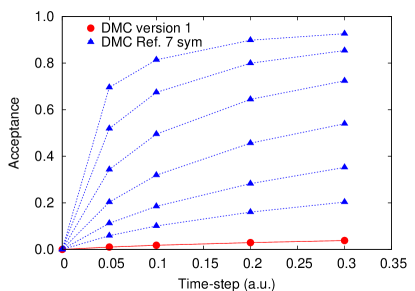
Figure 1: Acceptance of the $T_{\rm FN}^{\rm NL}$ move as a function of time-step. The increasing dotted curves correspond to systems with 1, 2, 4, 8, 16 and 32 oxygen atoms aligned at a distance of 30 $\AA$ from each other. The dotted curves are obtained with the algorithm of Ref. C06, while the lowest continuum curve is obtained with the size-consistent DMC algorithm (version 1) we propose. We only show the size-consistent curve with 1 atom as it is indistinguishable from the ones obtained for the larger systems.

To better understand the overall behavior of the algorithm with increasing system size, we also analyze the FN energy as a function of time-step. We are interested in comparing the results obtained with the conventional LA approach and with the algorithm of Ref. C06 described in the previous section. For a more meaningful and clear comparison with conventional DMC with the LA which employs a symmetrized branching factor, we modify the original algorithm as described in the previous section to also use a symmetrized branching factor:

$$\exp\left[-\tau\left(E_{\rm L}({\bf R})+E_{\rm L}({\bf R}^{\prime})\right)/2\right]$$ (16)

where ${\bf R}$ and ${\bf R}^{\prime}$ are the coordinates before the drift-diffusion move of the first electron and after the drift-diffusion move of the last electron, respectively, if the electrons are displaced subsequently. Such a simple modification is allowed as it only entails a different time-step error, which we actually find to be significantly smaller than the one obtained with the algorithm of Ref. C06 as we detail in the Section V.

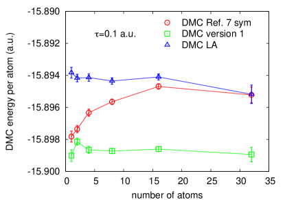
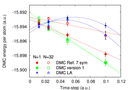
Figure 2: Upper panel: DMC FN energy per atom for systems of $M$ isolated oxygen atoms for $\tau=0.1$. For given time-step, the results of the algorithm of Ref. C06 (red circles) approach those of the LA (blue triangles) upon increasing the system size, whereas the present algorithm (DMC version 1, green squares) gives values independent of $M$. In the three algorithms, the branching factor is updated after having moved all the electrons (AE branching). Lower panel: time-step dependence of the DMC FN energy for the same three algorithms for $M=1$ (filled symbols) and $M=32$ (open symbols). The algorithm of Ref. C06 has a problematic extrapolation to zero time-step for large enough system size. For $M=32$, the linear extrapolation (red curve with open symbols) is consistent, as expected, with the corresponding result for $M=1$ (red curve with filled circles). However a better $\chi^{2}$ would be obtained with a quadratic extrapolation, which in turn would require a sudden upturn at very small $\tau$ to recover the correct zero time-step limit.

From the results reported in Fig. 2, we observe that the FN energies obtained with the algorithm of Ref. C06 significantly increase with $M$ and approach the energies obtained with the LA algorithm. Already with a system with 32 oxygen atoms, the FN energies at $\tau=0.1$ obtained with these two approaches become equivalent within the error bars. The energies given by the two algorithms must however extrapolate to different values as the time-step goes to zeroC06 . The lower panel of Fig. 2 shows that for $M=32$, in particular, they have to depart from each other within a tiny time-step interval near the origin. Because of this behavior, the algorithm of Ref. C06 is bound to have a problematic extrapolation to the zero time-step limit for large enough systems.

III.1 Size-consistent formulations: version 1

To address this problem, the original algorithm of Ref. C06 can be easily reformulated in a size-consistent manner by observing that the transition $T^{\rm NL}$ (Eq. 10) can be factorized as

$$T^{\rm NL}({\bf R}^{\prime},{\bf R},\tau) = \frac{\Psi_{\rm T}({\bf R}^{\prime})}{\Psi_{\rm T}({\bf R})}\prod_{i=1}^{N}\langle{\bf r}_{i}^{\prime}|e^{-\tau{\nu}^{\rm NL}}|{\bf r}_{i}\rangle$$ (17)

$$= \prod_{i=1}^{N}\frac{\Psi_{\rm T}({\bf r}^{\prime}_{1}\ldots{\bf r}^{\prime}_{i},{\bf r}_{i+1}\ldots)}{\Psi_{\rm T}({\bf r}^{\prime}_{1}\ldots{\bf r}^{\prime}_{i-1},{\bf r}_{i}\ldots)}\langle{\bf r}_{i}^{\prime}|e^{-\tau{\nu}^{\rm NL}}|{\bf r}_{i}\rangle$$

$$= \prod_{i=1}^{N}\left(\delta_{{\bf r}^{\prime}_{i}{\bf r}_{i}}-\tau v_{{\bf r}^{\prime}_{i}{\bf r}_{i}}\right)$$

$$= \prod_{i=1}^{N}t^{\rm NL}({\bf r}^{\prime}_{i},{\bf r}_{i},\tau)\,,$$

where $\nu^{\rm NL}$ is the non-local potential acting only on one electron due to all the atomic centers so that the total non-local potential is given by the sum over the electrons, $\langle{\bf R}^{\prime}|{\cal V}^{\rm NL}|{\bf R}\rangle=\sum_{i}\langle{\bf r}_{i}^{\prime}|{\nu}^{\rm NL}|{\bf r}_{i}\rangle$. We defined the matrix element $v_{{\bf r}^{\prime}_{i}{\bf r}_{i}}$ as

$$v_{{\bf r}^{\prime}_{i}{\bf r}_{i}}=\frac{\Psi_{\rm T}({\bf r}^{\prime}_{1}\ldots{\bf r}^{\prime}_{i},{\bf r}_{i+1}\ldots)}{\Psi_{\rm T}({\bf r}^{\prime}_{1}\ldots{\bf r}^{\prime}_{i-1},{\bf r}_{i}\ldots)}\langle{\bf r}_{i}^{\prime}|{\nu}^{\rm NL}|{\bf r}_{i}\rangle\,.$$ (18)

The transition $t^{\rm NL}({\bf r}^{\prime}_{i},{\bf r}_{i},\tau)$ displaces the $i$-th electron over the grid of quadrature points generated by considering only the $i$-th electron and all pseudoatoms which host the $i$-th electron in their core region.

The FN approximation is applied separately to each single-electron transition as

$$t_{\rm FN}^{\rm NL}({\bf r}^{\prime},{\bf r},\tau)=\delta_{{\bf r}^{\prime}{\bf r}}-\tau v^{-}_{{\bf r}^{\prime}{\bf r}}\,,$$ (19)

where $v^{\pm}_{{\bf r}^{\prime}{\bf r}}$ is defined in analogy to the case of the total non-local potential so that only the positive transition elements are kept in the transition matrix. In this formulation, the third step of the DMC algorithm detailed above consists of a loop over the electrons where each electron is subsequently moved according to the single-electron transition, $t_{\rm FN}^{\rm NL}$. Therefore, while in the original algorithm of Ref. C06 the configuration generated in the $T_{\rm FN}^{\rm NL}$ step differs from the starting configuration only in the coordinate of one electron, the configuration resulting from this size-consistent move will generally change in more than one electronic coordinate and the number of electrons being moved will increase with the size of the system.

To understand that the drift-diffusion-branching steps in the original algorithm do not need to be modified, we observe that the expression of the effective Hamiltonian ${\cal H}_{\rm eff}$ we are working with is the same as in Eq. 13 in the limit of $\tau$ going to zero. In particular, the sign-flip term obtained by summing all discarded terms $v^{+}_{{\bf r}^{\prime}{\bf r}}$ over all the electrons is equal to the sign-flip term in ${\cal V}_{\rm eff}^{\rm loc}$ (Eq. 12) to zero-order in $\tau$. Similarly, we have that, to order $\tau$,

$$\prod_{i=1}^{N}\sum_{{\bf r}^{\prime}_{i}}t_{\rm FN}^{\rm NL}({\bf r}^{\prime}_{i},{\bf r}_{i},\tau)\approx\sum_{{\bf R}^{\prime}}T_{\rm FN}^{\rm NL}({\bf R}^{\prime},{\bf R},\tau)\,,$$ (20)

and we recover the same branching factor as in the original algorithm. Therefore, both algorithms extrapolate to the same limit at zero time-steps. We will refer to this improved algorithm as “DMC version 1”, to distinguish it from another size-consistent version we will define later in this section. We stress here that by “version 1” we do not only mean the use of the product of single-particle $t_{\rm FN}^{\rm NL}$ in step 3, but also the symmetrization of the weights in step 2, as described in Eq. 16, where the initial configuration is taken before the diffusion process (step 1), and the final is the one after step 1.

The acceptance as a function of time-step using the size-consistent DMC algorithm (version 1) is shown in Fig. 1. We only report the result obtained with $M=1$ as the curves for the other system sizes are exactly equivalent within statistical error. This finding can be easily understood since the probability of moving a given electron on the grid generated by considering all centers will be practically the same as the probability computed using only the atom close to the electron as all other centers are at least 30 $\AA$ far apart. Therefore, in the new size-consistent algorithm, when more atoms are added to increase the size of the system, the loop over the electrons will ensure that each electron attempts a move around its closest center. The acceptance remains therefore constant as more oxygen atoms are added. In a more realistic systems (e.g. with closer oxygen atoms), there will be a weak dependence on the size of the system but, after enough atoms have been added for most electrons to experience an equivalent environment, the acceptance will become independent on the system size given the short-range nature of the non-local components of the pseudopotentials.

The FN energies obtained for the oxygen systems with this size-consistent algorithm are compared in Fig. 2 with the results of the LA and of the original algorithm. We observe that, as expected, the FN energies of the size-consistent algorithm extrapolate to the same value as the original algorithm as $\tau$ goes to zero. On the other hand, while the size-consistent FN energies are close to the values obtained with the original method for the smallest, one-atom system, the FN results obtained by the two methods depart from each other as the system size increases. Importantly, the FN energies of the size-consistent scheme do not approach the LA results for large systems at finite $\tau$ and their extrapolation to zero time-step is therefore as smooth for large as for small systems.

III.2 Size-consistent formulations: version 2

An alternative scheme to address the size-consistent problem of the original algorithm of Ref. C06 can be obtained through a different route by starting from Eq. 10, and breaking it up in $N$ terms with time-step of $\tau/N$, such that:

$$\sum_{{\bf R}^{\prime}}T_{\rm FN}^{\rm NL}({\bf R}^{\prime},{\bf R},\tau)=\sum_{{\bf R}_{1}\cdots{\bf R}_{N}}\prod_{i=1}^{N}T_{\rm FN}^{\rm NL}({\bf R}_{i},{\bf R}_{i-1},\tau/N)\,,$$ (21)

with ${\bf R}_{N}={\bf R}^{\prime}$, ${\bf R}_{0}={\bf R}$, and the sum over the quadrature points sampled by the chain $\{{\bf R}_{0},\ldots,{\bf R}_{i},\ldots,{\bf R}_{N}\}$ generated during the random walk. This is another way to evaluate the quantity in Eq. 20. The difference is that Eq. 21 involves a product of $N$ all-electron factors, while Eq. 20 is a factorization of $N$ single-electron terms. Both will avoid the saturation of the acceptance probability of the non-local Green’s function $T_{\rm FN}^{\rm NL}$, and therefore they will ensure a size-consistent time-step error. Since Eq. 21 requires the calculation of all matrix elements $V_{{\bf R}^{\prime},{\bf R}}$ each time, it is more convenient to split the $N$ factors in such a way that the diffusion move involving the $i$-th electron could be placed between the $i-1$-th and $i$-th factor, and the corresponding branching weight updated as a product of subsequent single-electron components:

$$\prod_{i=1}^{N}\,\exp\left[-\frac{\tau}{N}E_{\rm L}({\bf r}^{\prime}_{1}\ldots{\bf r}^{\prime}_{i},{\bf r}_{i+1}\ldots,{\bf r}_{N})\right]\,,$$ (22)

where we can exploit the knowledge of $V_{{\bf R}^{\prime},{\bf R}}$ to compute also $E_{\rm L}$ for every single-electron move. We will call this algorithm “DMC version 2” rqmc . It consists of the following steps:

• Diffusion move of the $i-$th electron.

• The weight of the walker is multiplied by the branching factor $\exp\left[-\frac{\tau}{N}E_{\rm L}({\bf r}^{\prime}_{1}\ldots{\bf r}^{\prime}_{i},{\bf r}_{i+1}\ldots,{\bf r}_{N})\right]$.

• The walker moves to ${\bf R}^{\prime\prime}$ according to the transition probability $T^{\rm NL}_{\rm FN}({\bf R}^{\prime\prime},{\bf R}^{\prime},\tau/N)/\sum_{{\bf R}^{\prime\prime\prime}}T_{\rm FN}^{\rm NL}({\bf R}^{\prime\prime\prime},{\bf R}^{\prime},\tau/N)$ which involves all the electrons.

In contrast to the original algorithm, and the “DMC version 1”, these three steps need to be performed inside a loop over the electrons. In the “version 2” formulation of the DMC size-consistent algorithm, each electron drifts and diffuses in a time $\tau$ and the branching factor is updated at each SE move with the total local energy $E_{\rm L}$ and time $\tau/N$ in the exponent. After each SE branching update, a non-local transition is performed with $T^{\rm NL}_{\rm FN}({\bf R}^{\prime},{\bf R},\tau/N)$, where one electron among all electrons is displaced over the grid of quadrature points obtained by considering all electrons and all pseudoatoms. Therefore, the electron displaced in the non-local move may differ from the electron which is currently being moved in the drift-diffusion step.

IV LRDMC and non-local pseudopotentials

The main difference between the effective DMC Hamiltonian reported in Eq. 13 and the LRDMC one is the kinetic operator ${\cal K}$. In the LRDMC approach, ${\cal K}$ is replaced by a discretized Laplacian and treated on the same footing as ${\cal V}^{\rm NL}$. In the original formulation, the discretized Laplacian is a linear combination of two discrete operators with incommensurate lattice spaces $a$ and $a^{\prime}$, introduced to sample densely the continuous space by performing discrete moves whose length is either $a$ or $a^{\prime}$. This method can be simplified by noticing that all the continuous space can be visited using only a single displacement length $a$, provided we randomize the direction of the Cartesian coordinates each time the electron positions are updated. The randomization of the lattice mesh is similar to the well established approach used to perform the angular integration in the non-local part of the pseudopotential fahy . Therefore, in the LRDMC approach, we can extend the definition of the kinetic part by including both the discretized Laplacian and the non-local part of the pseudopotentials. The total non-local operator reads:

$${\cal K}^{a}=-\sum\limits_{i=1}^{N}\Delta^{a}_{i}(\theta_{i},\phi_{i})/2+{\cal V}^{NL}\,,$$ (23)

where $\Delta^{a}_{i}(\theta_{i},\phi_{i})$ is the Laplacian acting on the $i$-th electron and discretized to second order so that $\Delta^{a}_{i}(\theta_{i},\phi_{i})=\Delta_{i}+O(a^{2})$. The discretized Laplacian is computed in a frame rotated by the angles $\theta_{i}$ and $\phi_{i}$, which are chosen randomly and independently of the ones used to compute ${\cal V}^{NL}$. In this formulation, we need to evaluate only 6 off-diagonal elements of the Green’s function instead of 12 as in the original algorithm, gaining a speed-up of a factor of 2 in full-core calculations and of ${(12+\mathrm{n_{\mathrm{quad}}})}/{(6+\mathrm{n_{\mathrm{quad}}})}$ with pseudopotentials, where $\mathrm{n_{\mathrm{quad}}}$ is the number of quadrature points per electron heavy . We notice that, with this simplification, the LRDMC error in the extrapolation to the continuous limit depends on a single parameter $a$, and the method can therefore be compared fairly with the DMC approach where the discretization of the diffusion process also depends on a single scale, i.e. the time-step $\tau$.

In the LRDMC choice of the Hamiltonian, we further regularize the single-particle operator ${\nu}$, defined as the electron-ion Coulomb interaction in full-core atoms or the local part ${\nu}^{\rm loc}$ of the pseudopotential, so that ${\nu}({\bf r}_{i})\to{\cal V}_{i}^{a}({\bf R})$ as

$${\cal V}_{i}^{a}({\bf R})={\nu}({\bf r}_{i})-{\frac{(\Delta_{i}-\Delta_{i}^{a})\Psi_{T}({\bf R})}{2\Psi_{T}({\bf R})}}\,,$$ (24)

when acting on the $i$-th electron. The single-particle operator ${\nu}$ acquires therefore a many-body term and ${\cal V}_{i}^{a}({\bf R})$ depends on the all-electron configuration ${\bf R}$. The total potential term is then given by

$${\cal V}^{a}=\sum\limits_{i=1}^{N}{\cal V}_{i}^{a}+{\cal V}_{ee}+{\cal V}_{nn}\,,$$ (25)

where no regularization is employed in the electron-electron ${\cal V}_{ee}$ and ion-ion ${\cal V}_{nn}$ Coulomb terms. This lattice regularization leads to an approximate Hamiltonian ${\cal H}^{a}={\cal K}^{a}+{\cal V}^{a}$ which converges to the exact Hamiltonian as ${\cal H}^{a}={\cal H}+a^{2}\Delta{\cal H}$ for $a\to 0$, where we denote with $a^{2}\Delta{\cal H}$ the $O(a^{2})$ LRDMC error on ${\cal H}$.

The lattice Green’s function Monte Carlo algorithm can then be employed to sample exactly the lattice regularized Green’s function, $\Lambda-{\cal H}^{a}$, and project the trial wave function $\Psi_{T}$ to the approximate ground state $\Psi_{a}^{\mathrm{LRDMC}}$ which fulfills the fixed-node constraint based on $\Psi_{T}$, in complete analogy to the DMC framework CFS05 . Note that, since the spectrum of ${\cal H}^{a}$ is not bounded from above, we need to take the limit $\Lambda\rightarrow\infty$, which can be handled with no loss of efficiency as described in Ref. lambda, . The usual DMC Trotter breakup results in a time-step error, while the LRDMC formulation yields a lattice-space error, but both approaches share the same upper bound property and converge to the same projected FN energy in the limit of zero time-step and lattice-space, respectively.

Since the discretized Laplacian and the non-local potential are treated on the same footing, and the sampling of the Green’s function is based on a sequence of single-particle moves generated both from the Laplacian and the non-local part, the LRDMC is intrinsically size-consistent (in the sense previously discussed for the DMC algorithm), and no modification is necessary to make the lattice-space bias independent of the system size. It will depend however on the quality of the trial wave function in the way detailed below.

IV.1 Small $a^{2}$ correction for good trial function

The regularization of the potential (Eq. 24) in the definition of the lattice Hamiltonian ${\cal H}^{a}$ implies that the correction $\Delta{\cal H}$ satisfies:

$$\Delta{\cal H}|\Psi_{T}\rangle=0.$$ (26)

Using this property, we can estimate the leading-order error of the lattice regularization by simple perturbation theory as

$$E^{a} = E^{0}+a^{2}\langle\Psi_{0}^{\mathrm{LRDMC}}|\Delta{\cal H}|\Psi_{0}^{\mathrm{LRDMC}}\rangle$$ (27)

$$= E^{0}+a^{2}\langle\Psi_{0}^{\mathrm{LRDMC}}-\Psi_{T}|\Delta{\cal H}|\Psi_{0}^{\mathrm{LRDMC}}-\Psi_{T}\rangle$$

$$= E^{0}+O(a^{2}|\Psi_{0}^{\mathrm{LRDMC}}-\Psi_{T}|^{2})\,,$$

where $E^{a}$ is the expectation value of the Hamiltonian ${\cal H}^{a}$ on the approximate FN ground state $\Psi_{a}^{\mathrm{LRDMC}}$ and $E^{0}$ the estrapolated value as $a\rightarrow 0$. Thus, the approach to the continuous limit is particularly fast for good trial functions, namely for $\Psi_{T}$ close to the ground state solution, since $\Psi_{0}^{\mathrm{LRDMC}}$ is a state with lower energy than $\Psi_{T}$ and has to approach the ground state at least as $\Psi_{T}$ does. The leading corrections to the continuous limit are quadratic in the wave function error. This property is not easily generalized to the usual DMC method and, to our knowledge, has not been established so far.

IV.2 Well defined lattice regularization

As in any lattice model, the Hamiltonian ${\cal H}^{a}$ has a finite ground state energy only if the potential ${\cal V}^{a}$ is always limited from below. If ${\cal V}^{a}({\bf R}_{0})=-\infty$ for some configuration ${\bf R}_{0}$, the variational state $\Psi({\bf R})=\delta_{{\bf R},{\bf R}_{0}}$ will have unbounded negative energy expectation value and the ground state energy of ${\cal H}^{a}$ is not defined. Unfortunately, the regularized potential ${\cal V}^{a}({\bf R})$ in Eq. (24) is not bounded from below when ${\bf R}$ belongs to the $(3N-1)$-dimensional nodal surface ${\cal N}$ defined by the equation $\Psi_{T}({\bf R})=0$. To cure these divergences, we need to be able to establish when a configuration is close to the nodal surface. In the lattice regularized formulation, we can assign an electron position ${\bf r}_{i}$ to the nodal surface, i.e. ${\bf r}_{i}\in{\cal N}_{a}$, if $\Psi_{T}({\bf r}_{i}+a\vec{\mu})$ has the opposite sign of $\Psi_{T}({\bf r}_{i})$ for at least one of the six points used to evaluate the finite difference Laplacian (i.e. $\vec{\mu}$ is one of the six unit vectors $\pm\hat{x},\pm\hat{y}$ or $\pm\hat{z}$ of the reference frame randomly oriented according to the angles $\theta_{i}$ and $\phi_{i}$). ${\cal N}_{a}$ correctly defines the nodal surface ${\cal N}$ in the limit $a\to 0$.

With this definition of nodal surface, we can modify ${\cal V}_{i}^{a}$ so that it remains finite when ${\bf r}_{i}\in{\cal N}_{a}$:

$$\tilde{\cal V}_{i}^{a}({\bf R})=\left\{\begin{array}[]{cc}\mathrm{Max}\left[{\nu}({\bf r}_{i}),{\cal V}_{i}^{a}({\bf R})\right]&{\rm if}~{}{\bf r}_{i}\in{\cal N}_{a}\\ {\cal V}_{i}^{a}({\bf R})&{\rm otherwise}\end{array}\,.\right.$$ (28)

If ${\bf r}_{i}\notin{\cal N}_{a}$, we use the original LRDMC definition of ${\cal V}_{i}^{a}$ since ${\cal V}_{i}^{a}$ remains finite even when an electron approaches a nucleus for trial functions which satisfy the electron-ion cusp conditions. If ${\bf r}_{i}\in{\cal N}_{a}$, we need to distinguish two cases. If the electron is not close to a nucleus, the regularized ${\cal V}_{i}^{a}$ can diverge negatively while ${\nu}({\bf r}_{i})$ remains finite and, according to Eq. 28, the potential $\tilde{\cal V}_{i}^{a}$ coincides with $\nu$. If the electron is close to a nucleus in a full-core calculation, both ${\cal V}_{i}^{a}$ and ${\nu}({\bf r}_{i})$ diverge, so we need to further regularize ${\nu}({\bf r}_{i})$ in the right hand side of Eq. (28) and use an expression bounded from below. In this particular case, we choose to replace the divergent electron-ion contribution $-Z/|{\bf r}_{in}|$ in ${\nu}({\bf r}_{i})$ with $-Z/a$ whenever the electron-ion distance $|{\bf r}_{in}|<a$.

If we employ the regularized potential $\tilde{\cal V}^{a}$ in the Hamiltonian ${\cal H}^{a}$, we no longer satisfy Eq. (26) and, in principle, it is not possible to compute $E^{a}$ by averaging the local energy ${\cal H}\Psi_{\rm T}/\Psi_{\rm T}$. However, the use of $\tilde{\cal V}^{a}$ introduces only negligible errors in the computation of $E^{a}$ because the regularization is adopted only in a region of volume $S\times a$, where $S$ is the area of the nodal surface ${\cal N}$. Since both the trial and the LRDMC wave function vanish $\simeq a$ close to the nodal surface, the finite lattice error corresponds to averaging $({\cal H}^{a}-{\cal H})\Psi_{T}/\Psi_{T}(\propto a$) over $\Psi_{T}\Psi_{FN}(\propto a^{2}$) in a nodal region of extension $\propto a$. If we collect these contributions, we find that the present regularization introduces a bias in the nodal region which vanishes as $a^{4}$ for $a\to 0$ and is always negligible compared to the dominant contribution $O(a^{2}|\Psi_{0}-\Psi_{T}|^{2})$. Moreover, since the regularization in Eq. (28) acts independently on each electron, it does not affect the size-consistent character of the algorithm, and the energy of $N$ independent atoms at large distances is equal to $N$ times the energy of a single atom. Therefore, we did not perform any LRDMC calculations for the oxygen systems since the energy per atom as a function of $a$ is exactly independent of $N$.

V Performance of the proposed methods

An important point to address is the efficiency of our revised techniques. This involves not only the computational cost per Monte Carlo step, but also the elimination of the discretization error (in time or space, as appropriate) by extrapolation to the continuum limit. Indeed, a smaller and smoother bias enhances the overall efficiency, as does the knowledge of the leading term in the discretization parameter.

V.1 Time-step error

We study the time-step error on the FN energy computed with the various algorithms discussed above, using the Oxirane molecule (C₂H₄O) as a test case. Our aim here is in particular to assess the reduction of the time-step error with respect to the original algorithm C06 . In the DMC “version 1” this reduction is due to the symmetrization of the weights, while in the DMC “version 2” it is due to the update of the branching factor after single-electron moves. We employ non-local energy-consistent Hartree-Fock pseudopotentials BFD07 for the oxygen and the carbon atoms in combination with the corresponding cc-pVDZ basis sets, and construct two single-determinant Jastrow-Slater wave functions of different quality. The first wave function is built from B3LYP orbitals and a very simple electron-electron Jastrow factor of the form $b[1-\exp(-\kappa r_{ij})]/\kappa$, where $b=1/2$ or $1/4$ for antiparallel- and parallel-spin electrons, respectively. The parameter $\kappa$ is optimized in energy minimization and is equal to 1.91. The second wave function is characterized by a more sophisticated Jastrow factor comprising of electron-electron, and electron-nucleus terms, and all orbital and Jastrow parameters in the wave function are optimized in energy minimization.

The top panel of Fig. 3 shows results obtained with the simple wave function. Consistently with previous studies on the water molecule needs-water , the LA energies extrapolate to a lower value (not necessarily variational) than the original algorithm of Ref. C06 , with a smaller time-step error; symmetrization of the branching factor in the original algorithm is already sufficient to reduce the time-step error down to a value similar to that found in the LA. As expected, given the small size of the system considered, the original and the size-consistent algorithm give nearly identical results, as shown here for its version 1 with AE branching.

The main result shown in the top panel of Fig. 3 is the remarkable reduction of the time-step error obtained with a SE branching factor. The data shown in the Figure refer to version 2 of the size-consistent algorithm. We also mention, without reporting the data, that when the branching factor is updated after SE moves, the symmetrization of the local energy in the exponent does not improve the time-step error significantly.

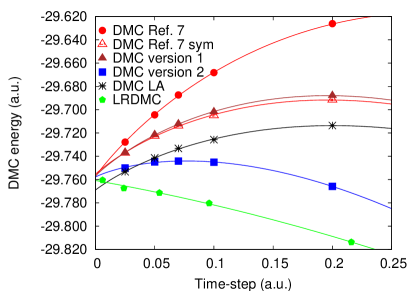
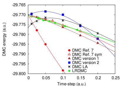
Figure 3: FN energies as a function of time-step for the Oxirane (C₂H₄O) molecule, obtained using a simple (top) and a more sophisticated (bottom) trial wave function. We employ different schemes, i.e. the original algorithm as in Ref. C06 and with an improved symmetrized branching factor (“sym”), the two size-consistent approaches we proposed (“DMC version 1”, and “DMC version 2”), the LA approach, and the LRDMC method. The lattice-space has been mapped into the time-step via the relation $\tau=0.6~{}a^{2}$, which guarantees the same autocorrelation time between the “DMC version 1” and the “LRDMC” method in this particular case.

The improvement obtained with a SE branching factor, however, is strongly dependent on the quality of the trial function. The lower panel of Fig. 3 shows results obtained with the more sophisticated wave function. We still find a lower energy with the LA (with its possibly problematic behavior at very small time-step), and a large time-step error with the original algorithm of Ref. C06 . All the other cases, however, display similar behavior, or at least comparable quality, in terms of the time-step error.

Also the LRDMC energy values are reported in Fig. 3, where the lattice-space has been converted into time-step based on the equal auto-correlation time between Monte Carlo generations in the DMC and LRDMC algorithms. This is the fairest mapping since it keeps the final statistical error equivalent for the same sample length. In this case, it gives $\tau\sim 0.6~{}a^{2}$. One can see that the LRDMC energies are always converging from below in a monotonic way, usually easier to extrapolate than the corresponding DMC energies.

In order to make a more quantitative analysis of the predictions reported in Section IV for the lattice-space error, we studied the lattice-space extrapolation of the Oxirane molecule with the DFT-B3LYP Slater determinant, and Jastrow factors going from the simple 2-body one, to the most complicated comprising of one-, two-, and three-body terms. The results are reported in Fig. 4. For good trial wave functions, a reliable extrapolation can be obtained even by using very large values of $a$, where small statistical errors can be obtained with much less computational effort. Also, the FN energies are basically independent of the shape of the trial wave function already for a rather simple Jastrow with 1-body and 2-body terms, implying that the “locality error” becomes negligible in the variational formulation even for not-so-accurate trial wave functions. This consideration applies also to the DMC variational energies, since the zero-lattice-space zero-time-step limits are equivalent.

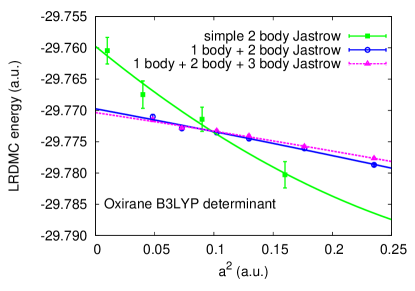
Figure 4: FN LRDMC energies as a function of lattice-space $a$ for the Oxirane (C₂H₄O) molecule, obtained using three types of Jastrow factors. The fitting curves include a quadratic and quartic term, namely $f(a)=E_{0}+ba^{2}+ca^{4}$. The finite lattice space error improves dramatically with a better wavefunction. For the simple 2-body Jastrow, $b\approx-0.15$, while for the most accurate Jastrow factor $b^{\prime}\approx-0.03$. The ratio of the variances of the two trial wave functions is roughly equal to $b/b^{\prime}$, in agreement with Eq. (27).

V.2 Relative efficiency

In all the methods presented here, there is an extra computational cost per Monte Carlo step with respect to the standard DMC with LA since an extra step is needed in order to sample correctly the Green’s function related to the non-local pseudopotentials. However, we have seen that, in all the variational methods, the non-local pseudopotential operator will displace only one electron a time since the non-local pseudopotential gives a one-body contribution to the Hamiltonian. This means that, in order to update all the quantities needed by the simulation as the wave function ratios, $V_{{\bf R}^{\prime},{\bf R}}$, the gradients and Laplacian terms, one can exploit the Sherman-Morrison algebra, which scales as $N^{2}$. For instance, to update the non-local term $V_{{\bf R}^{\prime},{\bf R}}$, as well as the ${\cal K}^{a}$ in the LRDMC, one employs the same algebra as the one used to update the gradient (i.e. the drift term) in the standard DMC with importance sampling. After a single particle move, the cost to fully update $V_{{\bf R}^{\prime},{\bf R}}$ scales as $\mathrm{n_{\mathrm{off}}}~{}N^{2}$ where $\mathrm{n_{\mathrm{off}}}$ is the number of non-local mesh points per electron ($\mathrm{n_{\mathrm{off}}}=\mathrm{n_{\mathrm{quad}}}$ in DMC with non-local pseudopotentials and $\mathrm{n_{\mathrm{off}}}=\mathrm{n_{\mathrm{quad}}}+6$ in LRDMC with non-local pseudopotentials and a single lattice-space in the Laplacian). In the size-consistent DMC (both “version 1” and “version 2”), the pseudopotential move has to be performed $N$ times in a single time-step $\tau$, so the overall cost per time-step coming from the pseudopotential operator is $\eta~{}\mathrm{n_{\mathrm{off}}}~{}N^{3}$, where $\eta$ is the acceptance ratio of the non-local part. Since $\mathrm{n_{\mathrm{off}}}\approx 20$, and $\eta\approx 0.1$ at convergence (see Fig. 1), it is clear that the DMC “version 1” will be only a prefactor $\approx 2$ slower than the standard DMC with LA. The “version 2” might be slightly slower than the “version 1” since it requires the calculation of the local energy after each single-particle move, but again the difference will be just a prefactor. The LRDMC approach is the slowest because the total number of operations in a cycle with $N$ single-electron updates of the local energy takes $(10+\mathrm{n_{\mathrm{quad}}})/(4+\mathrm{n_{\mathrm{quad}}})\leq 2.5$ more operations (the worst case is for full-core calculations when $\mathrm{n_{\mathrm{quad}}}=0$). Moreover, there is also an additional slowing down compared to the DMC “version 1” approach because, in the latter case, all operations involving the local energy can be done at the end of a cycle and cast in a very efficient form using matrix-matrix multiplications of size $\sim N$. These operations, for large $N>\simeq 1000$, can be much more efficient than single-electron matrix updates (by a factor ranging from 2 to 20, depending on the computer hardware and software). At present, it is difficult to estimate how much slower LRDMC will be on a particular machine efficiency_LRDMC , also considering that further algorithmic and software developments are expected in the near future, which should allow faster updates. However, even though LRDMC is certainly slower, it has the advantage of a much smoother lattice-space extrapolation as discussed above.

VI Conclusions

In conclusion, we have introduced important developments in the DMC and LRDMC methods in the context of electronic structure simulations with non-local pseudopotentials.

We have explained how to modify the DMC variational formulation for non-local potentials of Ref. C06 in order to make it size-consistent. We have shown that, for large systems, the original algorithm C06 will depart from the usual localization approximation only for small time-steps, making the zero time-step extrapolation possibly problematic. Instead, the two DMC algorithms presented here, based on a more accurate Trotter break-up for the non-local operator and a better branching factor, have a smaller and size-consistent time-step error. The DMC version 1, which features a single-particle representation of the non-local operator and a branching factor symmetric with respect to the application of the diffusion operator, is straightforward to implement in the existing codes. The DMC version 2 is closer to the LRDMC spirit, since the non-local part is further split in $\tau/N$ factor always acting on the all-electron configuration, and the branching factor is accumulated after every single-particle move. The latter version can give an even better time-step error (order $O(\tau/N)$ in the non-local part), particularly for relatively poor wave functions. In general, it is slightly more time consuming than the version 1, since it requires the evaluation of the full non local matrix after every single-particle move.

We have made significant progress also in the LRDMC approach. In the present formulation, it is no longer necessary to use two lattice meshes to randomize the electron position, but a single lattice space $a$ is sufficient, provided the orientation of the Cartesian coordinates of the discretized Laplacian is changed randomly during the diffusion process. We have defined a better lattice regularization of the Hamiltonian in order to have always a potential bounded from below, with a cutoff depending on $a$. This leads to a well defined and size-consistent lattice-space extrapolation since, in the $a\rightarrow 0$ limit, we recover the variational expectation value of the continuous Hamiltonian with a lattice space error whose leading term is quadratic in $a$. Moreover, we showed that the prefactor of the $a^{2}$ term vanishes quadratically in $|\Psi_{0}-\Psi_{T}|$. Therefore, for good wave functions, the extrapolation to the $a\to 0$ limit is particularly rapid and smooth with a computational effort $\propto 1/a^{2}$. The DMC error appears instead to be less correlated to the quality of the guiding function and may display a turn-down behavior for small time-steps (observed here and elsewhere needs-water ), which makes the time-step extrapolation much harder than in the LRDMC lattice-space approach. Regarding the computational cost, the LRDMC approach is slower but the overall efficiency is comparable to the two variational and size-consistent DMC formulations presented here since LRDMC allows one to work with large values of $a$ due to the robust extrapolation to the zero lattice-space limit.

- (1) W. M. C. Foulkes, L. Mitas, R. J. Needs, and G. Rajagopal, Rev. Mod. Phys. 73, 33 (2001).
- (2) D. M. Ceperley, J. Stat. Phys. 43, 815 (1986).
- (3) B. L. Hammond, P. J. Reynolds, W. A. Lester, Jr., J. Chem. Phys. 87, 1130 (1987).
- (4) S. Fahy, X. W. Wang and Steven G. Louie, Phys. Rev. B 42, 3503 (1990).
- (5) L. Mitáš, E. L. Shirley and D. M. Ceperley, J. Chem. Phys. 95, 3467 (1991).
- (6) M. Casula, C. Filippi, and S. Sorella, Phys. Rev. Lett. 95, 100201 (2005).
- (7) M. Casula, Phys. Rev. B 74, 161102(R) (2006).
- (8) S. Sorella and L. Capriotti, Phys. Rev. B 61, 2599 (2000).
- (9) D. F. B. ten Haaf, H. J. M. van Bemmel, J. M. J. van Leeuwen, W. van Saarloos, and D. M. Ceperley, Phys. Rev. B51, 13039 (1995).
- (10) M. Burkatzki, C. Filippi, and M. Dolg, J. Chem. Phys. 126, 234105 (2007).
- (11) C. Filippi and C. J. Umrigar, J. Chem. Phys. 105, 213 (1996). As Jastrow correlation factor, we use the exponential of the sum of two fifth-order polynomials of the electron-nuclear (e-n) and the electron-electron (e-e) distances, respectively. The Jastrow factor is adapted to deal with pseudo-atoms, and the scaling factor is set to 0.8 a.u. for the oxygen systems and 0.5 a.u. for oxirane.
- (12) C. J. Umrigar, J. Toulouse, C. Filippi, S. Sorella, and R. G. Henning, Phys. Rev. Lett. 98, 110201 (2007).
- (13) The short-time propagator of DMC version 2 lends itself to an implementation of the Reptation quantum Monte Carlo method [S. Baroni and S. Moroni, Phys. Rev. Lett. 82, 4745 (1999)] with single-particle moves.
- (14) For heavy elements treated either as full-core atoms or with small-core pseudopotentails, the two-mesh discretization might remain a better choice since it allows a more efficient sampling of the different length scales in the core and valence regions.
- (15) I.G. Gurtubay and R.J. Needs, J. Chem. Phys. 127, 124306 (2007).
- (16) M. W. Schmidt, K. K. Baldridge, J. A. Boatz, S. T. Elbert, M. S. Gordon, J. H. Jensen, S. Koseki, N. Matsunaga, K. A. Nguyen, S. Su, T. L. Windus, M. Dupuis, J. A. Montgomery, J. Comput. Chem. 14, 1347 (1993).
- (17) The relative efficiency between LRDMC and “DMC version 1” within the same machine (Intel quad-core) and the same code turbo is less than a factor for the cases shown in this work.
- (18) S. Sorella, https://qe-forge.org/projects/turborvb/.