Statistics of subgap states in $s_{\pm}$ superconductors

Abstract

There is strong support in favor of an unusual $s_{\pm}$ superconducting state in the new iron-based superconductors, in which the gap parameter has opposite signs in different bands. In this case scattering between different bands by impurities has a pair-breaking effect and introduces states inside the gap. We studied the statistics of disorder-induced subgap states in $s_{\pm}$ superconductors due to collective effects of impurities. Numerically solving the two-band Bogolyubov equations, we explored the behavior of the density of states and localization length. We located the mobility edge separating the localized and delocalized states for the 3D case and the crossover between the weak and strong localization regimes for the 2D case. We found that the widely used self-consistent T-matrix approximation is not very accurate in describing subgap states.

The recent discovery of high-temperature superconductivity in the iron arsenide LaFeAsO_1-xF_x Kamihara followed by the discovery of several new classes of superconducting materials IronPnictides led to a major breakthrough in the field of superconductivity. The Fermi surface of these materials is composed of several electron and hole sheets located near different points of the Brillouin zone BandStruct , see Fig. 1a. There is theoretical reasoning in favor of an electronic origin of superconductivity and a unusual superconducting state in which the order parameter has opposite signs in different bands (s_± state).spm-state This scenario is supported by the observation of a resonant magnetic mode in the superconducting state by inelastic neutron scattering.ChristiansonNat08

In the s_±-state interband scattering due to potential impurities (see Fig. 1a) has a pair-breaking effect similar to magnetic impurities in conventional superconductors.AGZhETF60 ; ShibaPTP68 ; RusinovPZheTF68 Such impurities introduce states inside the gap known as Shiba-Rusinov states for the magnetic-impurities problem.ShibaPTP68 ; RusinovPZheTF68 ; BalatskyRMP06 This leads to a finite density of states (DoS) at zero energy and strongly influences the superconducting properties at low temperatures. Most iron pnictides are doped superconductors and disorder due to dopant atoms is unavoidable. Experimental properties of iron pnictides which may be explained by a finite DoS at the Fermi level due to pair-breaking disorder include the “residual” linear temperature dependence of the specific heat in the superconducting state SpecHeat and a quadratic temperature dependence of the London penetration depth at low temperatures. LonPenT2

Transport properties at low temperatures, such as thermal conductivity ThermCond and microwave surface resistance, are sensitive to localization state of the low-energy quasiparticles. A random impurity potential may localize quasiparticles within some energy range. For 3D superconductors we typically expect two regimes: (i) At small concentrations of impurities states at the Fermi level are localized and a mobility edge at a finite energy exists, similar to impurity bands in semiconductors; (ii) At sufficiently high impurity concentrations all states are delocalized. The critical impurity concentration depends on the scattering properties of the impurities. In the first regime, the localized states near zero energy contribute to the low-temperature behavior of the thermodynamic but not transport properties.

A standard analytical approach to describe collective effects of impurities in superconductors is the self-consistent T-matrix approximation (SCTM). For the Born limit, it was elaborated in the famous paper by Abrikosov and Gor’kovAGZhETF60 and was later generalized for strong scattering ShibaPTP68 . Most theoretical works on collective effects of impurities in superconductors are based on this approximation, see, e.g., the review [BalatskyRMP06, ]. While giving a qualitative description of the impurity band, the SCTM approximation has serious deficiencies. For small impurity concentrations it predicts a hard gap in the spectrum. In reality, the DoS is finite at all energies, it has an exponential tailLifshitzTail due to rare fluctuation configurations of impurities, similar to the Lifshitz tail in the impurity band of semiconductors. Another deficiency of the SCTM description is that it ignores localization properties of the states. Localization of quasiparticles in superconductors was studied for dirty d-wave superconductors LocQPdwave and for the mixed state of disordered s-wave superconductors LocQPvortex . To our knowledge, localization in the impurity band of superconductors with pair-breaking impurities was never studied.

Several recent papers address different aspects of the impurity-induced subgap states PreostiMuzPRB96 ; SengaJPSJ08 ; Matsumoto09 and their possible influence on properties of iron pnictides VorontsovPRB09 . Studies of collective impurity effects, however, do not go beyond the SCTM approach. Motivated by the importance of disorder-induced subgap states for the properties of iron pnictides and the absence of an accurate theoretical description of these states, we performed a detailed study of their statistical properties based on numerical calculations. We explore the behavior of the density of states for s_± superconductors as function of scattering parameters and impurity concentration and compare the results with the SCTM approach. We also explore localization properties of states in order to locate the mobility edge in the parameter space.

Our study is based on the two-band Bogolyubov equations for the two-component wave functions, $\hat{\Psi}_{\alpha}=\binom{u_{\alpha}}{v_{\alpha}}$,

$$\left(E\!-\!\hat{\varepsilon}_{\alpha}\hat{\tau}_{z}\!+\!\Delta_{\alpha}\hat{\tau}_{x}\right)\hat{\Psi}_{\alpha}(\mathbf{r})-\hat{\tau}_{z}\sum_{l,\beta}\delta(\mathbf{r}-\mathbf{R}_{l})U_{\alpha\beta}^{l}\hat{\Psi}_{\beta}(\mathbf{r})\!=\!0.$$

Here $\alpha$ is the band index, $\hat{\tau}_{i}$ are Pauli matrices in Nambu space, $\hat{\varepsilon}_{\alpha}=\xi_{\alpha}(\hat{\mathbf{k}})-\varepsilon_{F}\approx\mathbf{v}_{F,\alpha}(\hat{\mathbf{k}}-\mathbf{k}_{F,\alpha})$, $\Delta_{\alpha}$ are the gap parameters. We assume that $\Delta_{2}=-\Delta_{1}$. The last term in the equation describes the interaction with impurities. The interband scattering is described by the off-diagonal terms in the matrix $U_{\alpha\beta}^{l}$. For scattering between bands $1$ and $2$, separated by wave vector $\mathbf{Q}$ equal to half of the reciprocal-lattice vector, $U_{12}^{l}$ contains the factor $\exp(i\mathbf{QR}_{l})$ which only takes values $\pm 1$ depending on $\mathbf{R}_{l}$. This means that even for identical impurities $U_{12}^{l}$ has random signs and its average is zero. We neglect inhomogeneities of the gap parameters due to impurities. It is known that these inhomogeneities are small and do not influence the quasiparticle states much. The key parameter of an isolated pair-breaking impurity is the energy of a localized stateMatsumoto09 , $E_{0}/\Delta\equiv\varepsilon_{0}=\sqrt{1-4\Gamma_{\mathrm{eff}}}$, where we introduced the effective interband scattering parameter,

$$\Gamma_{\mathrm{eff}}\!=\!\frac{\gamma_{12}\gamma_{21}}{1\!+\!\gamma_{22}^{2}\!+\!\gamma_{11}^{2}\!+\!2\gamma_{12}\gamma_{21}\!+\!\left(\gamma_{22}\gamma_{11}\!-\!\gamma_{12}\gamma_{21}\right)^{2}},$$ (1)

with $\gamma_{\alpha\beta}=\pi\nu_{\alpha}U_{\alpha\beta}$ being the reduced scattering amplitudes and $\nu_{\alpha}\!=\!\int\!\frac{d^{d}\mathbf{k}}{(2\pi)^{d}}\delta(\xi_{\alpha}(\mathbf{k})\!-\!\varepsilon_{F})$ being the normal DoS (per spin) for band $\alpha$.

We explore the properties of the subgap states for the two- and three-dimensional cases. For the numerical analysis, we rewrite the equations in a form containing only wave functions at the impurity sites,

$$\hat{\Psi}_{\alpha}(\mathbf{R}_{l})=\sum_{\beta,l^{\prime}}\hat{g}_{\alpha}(\mathbf{R}_{l}-\mathbf{R}_{l^{\prime}})\hat{\tau}_{z}\gamma_{\alpha\beta}^{l^{\prime}}\hat{\Psi}_{\beta}(\mathbf{R}_{l^{\prime}}),$$ (2)

where the reduced Green’s function is defined as

$$\hat{g}_{\alpha}(\mathbf{R})=\frac{1}{\pi\nu_{\alpha}}\int\frac{d^{d}\mathbf{k}}{(2\pi)^{d}}\exp(i\mathbf{kR})\frac{E+\varepsilon_{\alpha}(\mathbf{k})\hat{\tau}_{z}-\Delta_{\alpha}\hat{\tau}_{x}}{E^{2}-\varepsilon_{\alpha}^{2}(\mathbf{k})-\Delta_{\alpha}^{2}}$$

and $d$ is the spacial dimensionality.

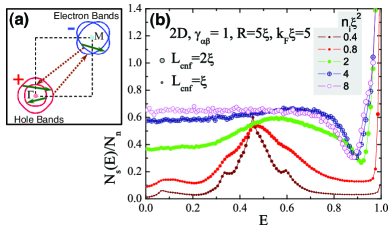
Figure 1: (color online)(a)The schematic band structure of iron pnictides. Solid and dotted arrows illustrate intraband and interband scattering events. (b)Evolution of the 2D subgap DoS with increasing concentration of impurities $n_{i}$ for isotropic scattering. Symbol sizes are proportional to $L_{\mathrm{cnf}}$ (3).

For each impurity realization inside a box of size $R^{d}$ we find the set of eigenenergies $E_{\lambda}$ and the corresponding four-component wave functions $\hat{\Psi}_{l}^{\lambda}\!=\![\hat{\Psi}_{1}^{\lambda}(\mathbf{R}_{l}),\hat{\Psi}_{2}^{\lambda}(\mathbf{R}_{l})]$, see appendix B. From the set of eigenenergies, we compute the average DoS, $N_{s}(E)=\left\langle\sum_{\lambda}\delta(E-E_{\lambda})\right\rangle$, where the average is taken over many impurity realizations. We normalize $N_{s}(E)$ to the total normal DoS for excitations, $N_{n}=4\nu$. To characterize localization properties, we compute the average confinement length for given energy,

$$L_{\mathrm{cnf}}(E,R)=\left\langle\sqrt{\sum_{a=x,y[,z]}\left(\left\langle r_{a}^{2}\right\rangle_{\lambda}-\left\langle r_{a}\right\rangle_{\lambda}^{2}\right)}\right\rangle_{E_{\lambda}=E},$$ (3)

where $\left\langle r_{a}^{m}\right\rangle_{\lambda}\!=\!\sum_{l}R_{l,a}^{m}|\Psi_{l}^{\lambda}|^{2}$ ($m\!=\!1,2$), and $|\Psi_{l}^{\lambda}|^{2}\!=\!\sum_{\alpha}\left[|u_{\alpha}^{\lambda}(\mathbf{R}_{l})|^{2}\!+\!|v_{\alpha}^{\lambda}(\mathbf{R}_{l})|^{2}\right]$. The behavior of $L_{\mathrm{cnf}}(E,R)$ with increasing system size, $R$, determines the nature of the states. For delocalized states $L_{\mathrm{cnf}}(E,R)$ is limited by the system size and linearly grows with $R$. For localized states $L_{\mathrm{cnf}}(E,R)$ saturates at a finite value, which gives the average localization length of states with energy $E$, $\lim_{R\rightarrow\infty}L_{\mathrm{cnf}}(E,R)=L_{\mathrm{loc}}(E)$.

We study the subgap densities of states at different concentrations of impurities and scattering parameters. We consider first the case of isotropic scattering, when all matrix elements $\gamma_{\alpha\beta}$ are equal. Figure 1b shows the evolution of the subgap DoS with increasing concentration of impurities $n_{i}$ for a moderate scattering rate, $\gamma_{\alpha\beta}=1$ for all $\alpha$ and $\beta$, and the system size $R=5\xi$. The energy is normalized to the gap value $\Delta$ and the coherence length is defined as $\xi=v_{F}/\Delta$. For small concentrations of impurities the DoS has a peak near the energy of the localized state. With increasing impurity concentrations, the peak broadens and becomes completely smeared already at relatively small impurity concentration $n_{i}\xi^{2}=2$. At higher concentrations the DoS becomes almost constant and comparable with the normal DoS.

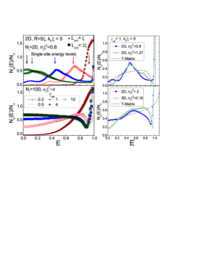
Figure 2: (color online) Left: Evolution of the subgap DoS with changing scattering rate for isotropic scattering for two impurity concentrations. Symbol sizes are proportional to the confinement length. Right: Comparison of the DoS shapes for the 2D and 3D models with identical pair-breaking parameters and SCTM results for two impurity concentrations.

The left part of Fig. 2 shows the subgap DoS for two impurity concentrations for a wide range of isotropic scattering rates. The energy location of the peak for small concentrations goes down with increasing scattering strength, while the maximum DoS is almost independent on $\gamma_{\alpha\beta}$. The peak smears with increasing impurity concentration and the magnitude of the density of states at large concentrations depends only weakly on the scattering strength for $\gamma_{\alpha\beta}>0.5$. Also, for large scattering rates the DoS approaches a limiting shape corresponding to the unitary limit. For small scattering strength, $\gamma_{\alpha\beta}=0.2$, we found the typical “Lifshitz tail” behavior.

Within the SCTM approximation (see appendix A) the DoS does not depend on dimensionality of superconductor, it is determined by the location of the single-site energy level and the pair-breaking parameter proportional to the impurity concentration $\alpha=2n_{i}\Gamma_{\mathrm{eff}}/(\pi\nu\Delta)$. Even though the overall evolution of the DoS shape with variations of the scattering strength and impurity concentration is similar in the 2D and 3D cases, the universality suggested by the SCTM approach does not exist. In the right part of Fig. 2 we compare the computed DoS for two impurity concentrations corresponding to the same pair-breaking strength in the 2D and 3D cases with the SCTM results. One can see that the DoS shapes for the two dimensionalities are similar but not identical. One noticeable difference is that the 3D DoS is typically smaller at low energies. The SCTM approximation does not reproduce the DoS shape at low impurity concentrations, the sharp peak in the center and the small features at the sides are not reproduced. These features appear due to the oscillating dependence of the impurity pair energy on their separation and correspond to the pairs separated by the distance at which the energies have extrema (see appendix C). For large impurity concentration we found a pronounced dip in the DoS for energies slightly smaller than $\Delta$, also not reproduced by the SCTM approximation.

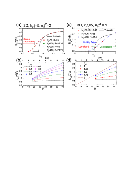
Figure 3: (color online) Plots (a) and (c) show the dependences of the zero-energy DoS on the scattering strength for isotropic scattering for 2D and 3D cases. Solid lines show the SCTM results. Plots (b) and (d) show the size dependences of the confinement length at different scattering strength.

We now focus on the region near zero energy, which determines the low-temperature behavior of the superconducting parameters. Figures 3(a,c) show the dependences of the zero-energy DoS on the isotropic scattering strength for fixed impurity concentration for the 2D and 3D models. We see that the DoS has a negligible size effect even at the smallest studied sizes. The SCTM approximation only roughly reproduces the the shape of the numerical curves and does not describe the tail region. The size dependences of the confinement length are shown in Fig. 3(b,d). We can see that for the 2D case at $\gamma_{\alpha\beta}<0.6$ the confinement length saturates at large $R$ approaching a finite localization length. No clear saturation of $L_{\mathrm{cnf}}$ is observed for $\gamma_{\alpha\beta}>0.6$. This may imply that states are delocalized or the localization length may be much larger than the studied system sizes. The second possibility looks more plausible, because for 2D disordered systems all electronic states are expected to be localized. The region $\gamma_{\alpha\beta}\approx 0.6$ probably marks a sharp crossover between the weak and strong localization regimes. We actually observe a noticeable downward curvature in the dependences of $L_{\mathrm{cnf}}$ vs. $R$ for all $\gamma_{\alpha\beta}$ which may be interpreted as a tendency towards localization at larger length scales. For the 3D case we expect a true mobility edge which we can estimate as the value of $\gamma_{\alpha\beta}$ at which $L_{\mathrm{cnf}}$ has a clear saturation tendency at large $R$. The estimated location of the mobility edge, $\gamma_{\alpha\beta}\approx 1.25$, is marked in Fig. 3c. It is close to the critical value bounding the SCTM gapped regions. We found that the DoS values at the mobility edge are quite small, ($\sim 0.02$ in our example). These values are significantly smaller than the DoS at the localization crossover for the 2D case. This observation implies that for identical bands in the 3D case there is only a very narrow parameter window within which the localized states at zero energy provide a noticeable DoS.

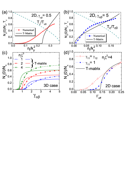
Figure 4: (color online) Plots (a) and (b) show the dependences of the zero-energy 2D DoS and transition temperature on concentration of impurities for two isotropic scattering rates. The clean-limit coherence length is taken as $k_{F}\xi\!=\!2.63$. (c)The dependences of the zero-energy 3D DoS on the scattering strength for three concentrations of impurities. (d)Densities of states as function of the interband scattering parameter $\Gamma_{\mathrm{eff}}$, Eq. (1), for two simulations series, isotropic scattering, $\gamma_{11}=\gamma_{12}$, and fixed intraband scattering amplitude, $\gamma_{11}=1$.

In figure 4(a,b) we compare the numerical and SCTM dependences of the zero-energy 2D DoS on the impurities concentration for weak and strong isotropic scattering. We also show the concentration dependences of the transition temperature evaluated using the Abrikosov-Gor’kov formula (see Ref. [AGZhETF60, ] and appendix A). For small scattering strength a noticeable DoS appears at the Fermi level only when $T_{c}$ is strongly suppressed. In contrast, for large scattering strength the DoS reaches values comparable with the normal DoS already at very minor suppression of $T_{c}$.

In Fig. 4c we present the dependences of the zero-energy DoS on the scattering strength for three concentrations of impurities, $n_{i}\xi^{3}=1$, $2$, and $4$ and compare them with the predictions of the SCTM approximation, which only coarsely reproduces the evolution of the DoS with increasing concentration. It does not describe the tail regions and systematically underestimates the value of the zero-energy DoS in the unitary limit, corresponding to large $\gamma_{\alpha\beta}$.

Up to this point we considered the case of isotropic scattering when all scattering amplitudes are equal. In general, one can expect that the interband scattering is always weaker than the intraband one. Within the SCTM approach the DoS is not sensitive to the individual scattering amplitudes and is completely determined by the parameter $\Gamma_{\mathrm{eff}}$, Eq. (1). To clarify the role of the relative strength of the scattering amplitudes, we study the subgap states for different interband amplitudes $\gamma_{12}=\gamma_{21}$ at fixed intraband amplitudes $\gamma_{11}=\gamma_{22}$. The DoS dependences on $\Gamma_{\mathrm{eff}}$ for the two simulation series are compared in Fig. 4d. We can see that the DoS is not simply determined by $\Gamma_{\mathrm{eff}}$, as suggested by the SCTM approach, but also sensitive to the relative strength of the intraband and interband scattering. For the same $\Gamma_{\mathrm{eff}}$ the DoS decreases with decreasing ratio $\gamma_{12}/\gamma_{11}$.

In conclusion, we explored the subgap DoS and localization properties for disordered s_± superconductors. We found that the widely-used analytical description (SCTM) is incomplete and not very accurate. Disorder makes superconductivity “gapless”, the DoS at $E=0$ is always finite. In the 3D case there is a mobility edge separating localized and delocalized states. It reaches zero energy at a critical impurity concentration above which all states become delocalized. In the 2D case the mobility edge is replaced by a crossover separating strongly and weakly localized states. The development of quantitative theory of the subgap states is crucial for the understanding properties of the iron pnictides and other superconductors with pair-breaking impurities.

We would like to thank I. Vekhter, T. Proslier, K. Matveev, and U. Welp for useful discussions. This work is supported by UChicago Argonne, LLC, under contract No. DE-AC02-06CH11357 and by the Center for Emergent Superconductivity, an Energy Frontier Research Center funded by the U.S. DOE, Office of Science, Office of BES under Award No. DE-AC0298CH1088

Appendix A Self-Consistent T-matrix approximation

The self-consistent T-matrix approximationShibaPTP68 is defined by the coupled equations for the average Green’s function $\hat{G}_{\alpha\beta}(\mathbf{k})\equiv\delta_{\alpha\beta}\hat{G}_{\alpha}(\mathbf{k})$ and the self-energy part $\hat{\Sigma}_{\alpha}\equiv\delta_{\alpha\beta}\hat{\Sigma}_{\alpha\alpha}$,

$$\hat{G}_{\alpha}(\mathbf{k})=\left[E-\hat{\varepsilon}_{\alpha}\hat{\tau}_{z}+\Delta_{\alpha}\hat{\tau}_{x}-\hat{\Sigma}_{\alpha}\right]^{-1},$$ (4a)

$$\hat{\Sigma}_{\alpha}=n_{i}\hat{T}_{\alpha}=n_{i}\left\langle\left(1-\hat{\tau}_{z}U_{\alpha\beta}\hat{G}_{0,\beta}\right)^{-1}\hat{\tau}_{z}U_{\beta\alpha}\right\rangle$$ (4b)

with $$\hat{G}_{0,\alpha}=\int\frac{d^{d}\mathbf{k}}{(2\pi)^{d}}\hat{G}_{\alpha}(\mathbf{k}) \hat{\Sigma}_{\alpha\beta} U_{\alpha\beta} N_{\alpha}(E)=\operatorname{Im}\left\{\mathrm{Tr}\left[\hat{G}_{0,\alpha}(E-i\delta)\right]\right\} \hat{\Sigma}_{\alpha}=\sum_{i}\Sigma_{\alpha,i}\hat{\tau}_{i} i=0,x,y,z N_{\alpha}(E) u_{\alpha}=\left(E-\Sigma_{\alpha,0}\right)/\left(\Delta-\Sigma_{\alpha,x}\right)$$. Note that the off-diagonal components of average to zero due to the random signs of the off-diagonal components of . The partial density of states is related to the Green’s function as . Using the expansion with , we can express via the ratio as

$$N_{\alpha}(E)=2\nu_{\alpha}\operatorname{Im}\frac{u_{\alpha}}{\sqrt{1-u_{\alpha}^{2}}}.$$ (5)

Here the factor $2$ accounts for the electron and hole excitations.

In the case of identical bands, this system reduces to an equation for only one complex parameter $u=\left(E-\Sigma_{0}\right)/\left(\Delta-\Sigma_{x}\right)$, similar to the Shiba equation for magnetic impuritiesShibaPTP68 ,

$$u\left(1-\alpha\frac{\sqrt{1-u^{2}}}{\varepsilon_{0}^{2}-u^{2}}\right)=\frac{E}{\Delta},$$ (6)

$$\alpha=\frac{2n_{i}\Gamma_{\mathrm{eff}}}{\pi\nu\Delta}=\frac{1}{\tau_{12}\Delta}$$ (7)

$$=\frac{2n_{i}}{\pi\nu\Delta}\frac{\gamma_{12}\gamma_{21}}{1+\gamma_{22}^{2}+\gamma_{11}^{2}+2\gamma_{12}\gamma_{21}+\left(\gamma_{22}\gamma_{11}-\gamma_{12}\gamma_{21}\right)^{2}}.$$

We observe that increasing the intraband scattering potential $\gamma_{\alpha\alpha}$ increases the intraband scattering time $\tau_{12}$ and diminishes the pair-breaking parameter $\alpha$.SengaJPSJ08 We also note that the SCTM results do not depend on dimensionality of the superconductor.

We summarize the most important analytical results obtained within this approximation. The SCTM approximation gives a gapped state for $\alpha<\varepsilon_{0}^{2}$ and gapless state for $\alpha>\varepsilon_{0}^{2}$ with finite total density of state at zero energy

$$N_{s}(0)=4\nu\frac{\sqrt{\alpha^{2}-\varepsilon_{0}^{4}}}{\sqrt{\frac{\alpha^{2}}{2}+\varepsilon_{0}^{2}\left(1-\varepsilon_{0}^{2}\right)+\alpha\sqrt{\frac{\alpha^{2}}{4}+1-\varepsilon_{0}^{2}}}}.$$ (8)

We stress again that the existence of a gapped state is unrealistic feature and deficiency of this approximation.

The suppression of $T_{c}$ is determined by the Abrikosov-Gor’kov formula AGZhETF60 ,

$$\ln\frac{T_{c0}}{T_{c}}=\psi(1/2+1/2\pi\tau_{12}T_{c})-\psi(1/2),$$ (9)

where $\psi(x)$ is the digamma function. This famous result is almost always understood too literally. In fact, it just gives an approximate typical value of the critical temperature. In real systems, due to the random arrangement of impurities, the transition temperature is inhomogeneous and the transition has percolative nature.

The average zero-temperature gap parameter is determined by the equations RusinovPZheTF68

$$\ln\frac{\Delta_{0}}{\Delta}=\frac{\pi}{2}\frac{\alpha}{1+\varepsilon_{0}}\text{ for }\alpha<\varepsilon_{0}^{2}$$ (10a)

with $$\alpha=\alpha_{0}\Delta_{0}/\Delta$$ and

$$\ln\frac{\Delta_{0}}{\Delta} =\frac{\pi}{2}\frac{\alpha}{\varepsilon_{0}+1}+\ln\left(u_{0}+\sqrt{1+u_{0}^{2}}\right)-\frac{\alpha u_{0}}{u_{0}^{2}\!+\!\varepsilon_{0}^{2}}$$

$$\!+\!\frac{\alpha}{\varepsilon_{0}^{2}\!-\!1}\left[\arctan u_{0}\!-\!\varepsilon_{0}\arctan\left(\frac{u_{0}}{\varepsilon_{0}}\right)\right],$$ (10b)

$$\text{with }u_{0}^{2}= \frac{\alpha^{2}}{2}-\varepsilon_{0}^{2}+\alpha\sqrt{\frac{\alpha^{2}}{4}+1-\varepsilon_{0}^{2}},\text{ for }\alpha>\varepsilon_{0}^{2}$$

Here $\Delta_{0}$ is the gap parameter for the clean case.

Appendix B Numerical simulations

To develop a precise theoretical description of the subgap region, we solve Eqs. (2) of the main paper numerically for the two-dimensional and three-dimensional cases. The main element of these equations is the Green’s function in real space, $\hat{g}_{\alpha}(r)$. At $r=0$ the Green’s function does not depend on dimensionality,

$$\hat{g}_{\alpha}(0)=\frac{-E+\Delta_{\alpha}\hat{\tau}_{x}}{\sqrt{\Delta_{\alpha}^{2}-E^{2}}}.$$

Large-$r$ asymptotics of $\hat{g}_{\alpha}(r)$ for $k_{F,\alpha}r\gg 1$ are given by

$$\hat{g}_{\alpha}(r) =\left[\frac{-E+\Delta_{\alpha}\hat{\tau}_{x}}{\sqrt{\Delta_{\alpha}^{2}-E^{2}}}\cos\left(k_{F,\alpha}r-\frac{\pi}{4}\right)-\hat{\tau}_{z}\sin\left(k_{F},_{\alpha}r-\frac{\pi}{4}\right)\right]\frac{\exp\left(-\sqrt{\Delta_{\alpha}^{2}-E^{2}}r/v_{F,\alpha}\right)}{\sqrt{\pi k_{F,\alpha}r/2}}\text{, for 2D case}$$

$$\hat{g}_{\alpha}(r) =\left[\frac{-E+\Delta_{\alpha}\hat{\tau}_{x}}{\sqrt{\Delta_{\alpha}^{2}-E^{2}}}\sin(k_{F,\alpha}r)-\hat{\tau}_{z}\cos(k_{F,\alpha}r)\right]\frac{\exp(-\sqrt{\Delta_{\alpha}^{2}-E^{2}}r/v_{F,\alpha})}{k_{F,\alpha}r}\text{, for 3D case}$$

As the probability to find two impurities at distance $\sim 1/k_{F}$ is very small, the structure of states is mostly determined by these asymptotics and the value at $r=0$. To match the large-$r$ asymptotics with the $r=0$ value, we use an approximate forms of the Green’s functions. For the 2D case we use

$$\hat{g}_{\alpha}(r) =\left[\frac{-E+\Delta_{\alpha}\hat{\tau}_{x}}{\sqrt{\Delta_{\alpha}^{2}-E^{2}}}J_{0}\left(k_{F,\alpha}r\right)+\hat{\tau}_{z}J_{1}\left(k_{F,\alpha}r\right)\right]$$

$$\times\exp\left(-\sqrt{\Delta_{\alpha}^{2}-E^{2}}r/v_{F,\alpha}\right),$$ (11)

where $J_{0}\left(x\right)$ and $J_{1}\left(x\right)$ are Bessel functions and for the 3D case we use

$$\hat{g}_{\alpha}(r) \!=\!\left[\frac{-E\!+\!\Delta_{\alpha}\hat{\tau}_{x}}{\sqrt{\Delta_{\alpha}^{2}\!-\!E^{2}}}\frac{\sin(k_{F,\alpha}r)}{k_{F,\alpha}r}-\hat{\tau}_{z}\mathcal{U}(k_{F,\alpha}r)\frac{\cos(k_{F,\alpha}r)}{k_{F,\alpha}r}\right]$$

$$\times\exp(-\sqrt{\Delta_{\alpha}^{2}-E^{2}}r/v_{F,\alpha})$$ (12)

with the interpolation function $\mathcal{U}(z)=z^{2}/(z^{2}+1)$. We expect that the exact behavior of the Green’s functions at $k_{F,\alpha}r\!\sim\!1$ not reproduced by these interpolations have little influence on the properties of the subgap states. In this paper we limit ourselves with the simplest case of two equivalent bands, meaning that $k_{F,1}=k_{F,2}\equiv k_{F}$, $v_{F,1}=v_{F,2}\equiv v_{F}$, and $\Delta_{1}=-\Delta_{2}\equiv\Delta$. The gap $\Delta$ is used as a unit of energy and $k_{F}^{-1}$ is used as a unit of length.

We employ the following numerical procedure. First, we define an impurity realization by $N_{i}$ random coordinates [$\mathbf{R}_{l}$] in a box, $0<R_{l,a}<R$, and random impurity signs $\delta_{l}=\pm 1$ for the off-diagonal scattering amplitudes, $U_{12}^{l}=\delta_{l}U_{12}$. From the linear $4N_{i}\times 4N_{i}$ system defined by Eq. (2) of the main paper, we find the eigenenergies, $E_{\lambda}$, and corresponding eigenstates $\Psi^{\lambda}(\mathbf{R}_{l})$. From the set of eigenenergies, $E_{\lambda}$, we compute the average density of state

$$N_{s}(E)=\left\langle\sum_{\lambda}\delta(E-E_{\lambda})\right\rangle,$$ (13)

where average is taken over many impurity realizations. Practically, this implies that for every realization we find the number of states $\Delta N(E)$ falling within the energy interval $[E-\Delta E/2,E+\Delta E/2]$ and then compute the average $N_{s}(E)=\langle\Delta N(E)/(\Delta ER^{2})\rangle$. As an isolated impurity generates one localized state, for small concentration of impurities the normalization condition $\int_{0}^{\Delta}N_{s}(E)dE=N_{i}/R^{2}$ is satisfied. We normalize $N_{s}(E)$ to the total normal density of states for excitations, $N_{n}=4\nu$, where for the 2D case the single-band DoS per electron is given by $\nu=k_{F}/(2\pi v_{F})$ and for the 3D case, $\nu=k_{F}^{2}/(2\pi^{2}v_{F})$.

To characterize localization properties, we also compute the average confinement length for states at given energy,

$$L_{\mathrm{cnf}}(E,R)=\left\langle\sqrt{\sum_{a}\left\langle\delta r_{a}^{2}\right\rangle_{\lambda}}\right\rangle_{E_{\lambda}=E},$$ (14)

where $a=x,y[,z]$ and the confinement length of state $\lambda$, $\left\langle\delta r_{a}^{2}\right\rangle_{\lambda}$, is determined by its wave function $\Psi_{l}^{\lambda}$ as

$$\left\langle\delta r_{a}^{2}\right\rangle_{\lambda} =\left\langle r_{a}^{2}\right\rangle_{\lambda}-\left\langle r_{a}\right\rangle_{\lambda}^{2},$$

$$\left\langle r_{a}\right\rangle_{\lambda} =\sum_{l}R_{l,a}|\Psi_{l}^{\lambda}|^{2},\ \ \left\langle r_{a}^{2}\right\rangle_{\lambda}=\sum_{l}R_{l,a}^{2}|\Psi_{l}^{\lambda}|^{2}$$

with $|\Psi_{l}^{\lambda}|^{2}\!=\!\sum_{\alpha}\left[|u_{\alpha}^{\lambda}(\mathbf{R}_{l})|^{2}\!+\!|v_{\alpha}^{\lambda}(\mathbf{R}_{l})|^{2}\right]$ and $\sum_{l}|\Psi_{l}^{\lambda}|^{2}\!=\!1$. The behavior of the confinement length with increasing system size, $R$, determines wether states at given energy are localized or not. For delocalized states, $L_{\mathrm{cnf}}(E,R)$ is limited by the system size and grows proportionally to $R$. For localized states, $L_{\mathrm{cnf}}(E,R)$ saturates at a finite value, which gives the average localization length of states with energy $E$, $\lim_{R\rightarrow\infty}L_{\mathrm{cnf}}(E,R)=L_{\mathrm{loc}}(E).$ In three dimensions for relatively small concentration of impurities one can expect the existence of a mobility edge in the subgap region separating localized and delocalized states. It is defined as the energy $E_{\mathrm{ME}}(n_{i},\gamma_{\alpha\beta})$ at which the localization length diverges, $L_{\mathrm{loc}}(E\!\rightarrow\!E_{\mathrm{ME}})\rightarrow\infty$. At a critical concentration of impurities depending on the scattering parameters, $n_{cr}(\gamma_{\alpha\beta})$, the mobility edge reaches zero energy, $E_{\mathrm{ME}}[n_{cr}(\gamma_{\alpha\beta}),\gamma_{\alpha\beta}]=0$, and all states become delocalized.

In the calculations of the concentration dependences presented in the Figs. 4a,b we took into account suppression of the average gap parameter described by Eqs. (10a) and (10b) and corresponding increase of the coherence length $\xi=v_{F}/\Delta$.

Appendix C Density of states at small concentration of impurities: pairs-dominated regime

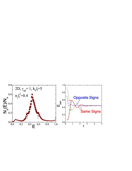
Figure 5: (color online) Left: The 2D DoS for small concentration of impurities, same as in Fig.1 of the main paper. Right: The energy of impurity pair as a function of the distance between impurities for same-sign and opposite-sign impurities. The arrows mark the extremum points which account for the small peaks in the DoS.

At small concentrations of impurities, $n_{i}\xi^{d}\ll 1$, the density of state is determined by impurity pairs.LifshitzPGBook The interaction between two close impurities gives the correction to the energyRusinovPZheTF68 , $E_{\mathrm{pair}}(r)=\varepsilon_{0}+\delta\varepsilon(r)$ and the behavior of the correction $\delta\varepsilon(r)$ depends on the relative sign of the off-diagonal scattering potential $U_{12}$ for two impurities. For same-sign impurities the single-site energy level splits into two levels corresponding to symmetric and antisymmetric combinations of the wave functions at the impurity sites. The separation-dependent energy corrections, $\delta\varepsilon_{\pm}$, rapidly oscillate with distance between the impurities $r$ as

$$\delta\varepsilon_{\pm}(r)\propto\pm\frac{\sin(k_{F}r+\alpha_{d})}{(k_{F}r)^{(d-1)/2}}\exp\left(-\sqrt{1-\varepsilon_{0}^{2}}r/\xi\right),$$

where $\xi=v_{F}/\Delta$ is the coherence length and $d$ is space dimensionality, see Fig. 5. For opposite-sign impurities the energy level remains double-degenerate with two states corresponding to localization near two impurity sites. The separation-dependent energy shift in this case is always positive and much smaller than for the same-sign impurities,

$$\delta\varepsilon(r)\propto\frac{\sin^{2}(k_{F}r+\alpha_{d})}{(k_{F}R)^{d-1}}\exp\left(-2\sqrt{1-\varepsilon_{0}^{2}}r/\xi\right).$$

The coefficients in the energy corrections depend on the scattering parameters of impurities.

The contribution to the DoS coming from impurity pairs with separation $r_{p}$ less than the typical distance, $r_{p}\ll n_{i}^{-d}$, can be evaluated in a simple way.LifshitzPGBook The concentration of the impurity pairs with separations between $r_{p}$ and $r_{p}+dr_{p}$ is given by $\frac{A_{d}}{2}n_{i}^{2}r_{p}^{d-1}dr_{p}$ with $A_{2}=2\pi$ and $A_{3}=4\pi$. The contribution to the DoS at the energy $E$ is given by the pairs satisfying the equation $E=E_{\mathrm{pair}}(r_{p})$ and for a nonmonotonic dependence $E_{\mathrm{pair}}(r)$, this equation may have several solutions. The pair contribution to the DoS can be evaluated as

$$N_{s}(E)=\frac{A_{d}}{2}n_{i}^{2}\sum_{r_{p}}\left[r_{p}(E)\right]^{d-1}\left|\frac{dr_{p}}{dE}\right|,$$

where the sum is taken over all values of $r_{p}$ corresponding to the same energy.

For pair separations corresponding to the energy extrema, $E_{\mathrm{pait}}(r)\approx E_{e}+\frac{a}{2}(r-r_{e})^{2}$, the isolated-pairs approximation gives a divergency at $E\rightarrow E_{e}$,

$$N_{s}(E)\approx\frac{A_{d}n_{i}^{2}\left[r_{e}\right]^{d-1}}{\sqrt{2a\left(E-E_{e}\right)}}.$$

These singularities, smeared by interactions with more remote impurities, account for the small peaks found in the DoS at small concentrations, see Fig. 5. The energy for opposite-sign impurities has a series of minima at exactly $E=\varepsilon_{0}$ meaning that there is also such a pair singularity at the peak center. This explains the sharpness of the peak at small concentrations of impurities.

References

- (1) Y. Kamihara, et al., J. Am. Chem. Soc. 130, 3296 (2008).
- (2) C.W. Chu, et al., Physica C 469, 326 (2009); D. Johrendt and R. Pöttgen, ibid, p. 332; M.K. Wu, et al., ibid, p. 340; A. S. Sefat, et al., ibid, p. 350; P.M. Shirage, et al., ibid, p. 355; J. Karpinski, et al., ibid, p. 370; X. Zhu, et al., ibid, p. 381.
- (3) D.J. Singh, Physica C, 469, 418 (2009); I.I. Mazin and J. Schmalian, ibid, p. 614.
- (4) I. I. Mazin, et al., Phys. Rev. Lett. 101, 057003 (2008); K. Kuroki, et al., Phys. Rev. Lett. 101, 087004 (2008).
- (5) A. D. Christianson, et al., Nature, 456, 930 (2008).
- (6) A. A. Abrikosov and L. P. Gor’kov, Zh. Eksp. Teor. Fiz., 39, 1781 (1960) [Sov. Phys. JETP 12, 1243 (1961)].
- (7) H. Shiba, Prog. Theor. Phys., 40, 435 (1968).
- (8) A. I. Rusinov, Pis’ma Zh. Eksp. Teor. Fiz. 9, 146 1968 [JETP Lett. 9, 85 (1969)]; Zh. Eksp. Teor. Fiz. 56, 2047 (1969) [Sov. Phys. JETP 29, 1101 (1969)].
- (9) A. V. Balatsky, I. Vekhter, and Jian-Xin Zhu, Rev. Mod. Phys. 78, 373 (2006).
- (10) J. K. Dong, et al., New Journal of Physics, 10, 123031 (2008); G. Mu, et al., arXiv:0906.4513.
- (11) C. Martin, et al., Phys. Rev. B 80, 020501 (2009); R. T. Gordon, et al., ibid, 79, 100506 (2009); K. Hashimoto, et al., Phys. Rev. Lett. 102, 207001 (2009).
- (12) Y. Machida, et al., arXiv:0906.0508; M. A. Tanatar, et al., arXiv:0907.1276.
- (13) A. Lamacraft and B. D. Simons, Phys. Rev. Lett. 85, 4783 (2000); Phys. Rev. B 64, 014514 (2001); A. V. Shytov, et al., Phys. Rev. Lett., 90, 147002 (2003).
- (14) T. Senthil, et al., Phys. Rev. Lett. 81, 4704 (1998); A. G. Yashenkin, et al., Phys. Rev. Lett., 86, 5982 (2001).
- (15) R. Bundschuh, et al., Phys. Rev. B, 59, 4382 (1999); S. Vishveshwara, et al., Phys. Rev. B, 61, 6966 (2000).
- (16) G. Preosti and P. Muzikar, Phys. Rev. B 54, 3489 (1996).
- (17) Y. Senga and H. Kontani, Journ. Phys. Soc. Jap. 77, 113710 (2008); arXiv:0812.2100.
- (18) M. Matsumoto, M. Koga, and H. Kusunose, J. Phys. Soc. Jpn., 78, 084718 (2009).
- (19) A. B. Vorontsov, et al., Phys. Rev. B 79, 140507(R) (2009); Y. Bang, EPL, 86, 47001 (2009).
- (20) I. M. Lifshits, S. A. Gredeskul, L. A. Pastur, Introduction to the theory of disordered systems, New York: Wiley, 1988.