A Study of the Effect of
Molecular and Aerosol Conditions in the Atmosphere
on Air Fluorescence Measurements at the
Pierre Auger Observatory

Abstract

The air fluorescence detector of the Pierre Auger Observatory is designed to perform calorimetric measurements of extensive air showers created by cosmic rays of above $10^{18}$ eV. To correct these measurements for the effects introduced by atmospheric fluctuations, the Observatory contains a group of monitoring instruments to record atmospheric conditions across the detector site, an area exceeding 3,000 km². The atmospheric data are used extensively in the reconstruction of air showers, and are particularly important for the correct determination of shower energies and the depths of shower maxima. This paper contains a summary of the molecular and aerosol conditions measured at the Pierre Auger Observatory since the start of regular operations in 2004, and includes a discussion of the impact of these measurements on air shower reconstructions. Between $10^{18}$ and $10^{20}$ eV, the systematic uncertainties due to all atmospheric effects increase from $4\%$ to $8\%$ in measurements of shower energy, and $4$ $\text{g~{}cm}^{-2}$ to $8$ $\text{g~{}cm}^{-2}$ in measurements of the shower maximum.

1 Introduction

The Pierre Auger Observatory in Malargüe, Argentina (69^∘ W, 35^∘ S, 1400 m a.s.l.) is a facility for the study of ultra-high energy cosmic rays. These are primarily protons and nuclei with energies above $10^{18}$ eV. Due to the extremely low flux of high-energy cosmic rays at Earth, the direct detection of such particles is impractical; but when cosmic rays enter the atmosphere, they produce extensive air showers of secondary particles. Using the atmosphere as the detector volume, the air showers can be recorded and used to reconstruct the energies, arrival directions, and nuclear mass composition of primary cosmic ray particles. However, the constantly changing properties of the atmosphere pose unique challenges for cosmic ray measurements.

In this paper, we describe the atmospheric monitoring data recorded at the Pierre Auger Observatory and their effect on the reconstruction of air showers. The paper is organized as follows: Section 2 contains a review of the observation of air showers by their ultraviolet light emission, and includes a description of the Pierre Auger Observatory and the issues of light production and transmission that arise when using the atmosphere to make cosmic ray measurements. The specifics of light attenuation by aerosols and molecules are described in Section 3. An overview of local molecular measurements is given in Section 4, and in Section 5 we discuss cloud-free aerosol measurements performed at the Observatory. The impact of these atmospheric measurements on the reconstruction of air showers is explored in Section 6. Cloud measurements with infrared cameras and backscatter lidars are briefly described in Section 7. Conclusions are given in Section 8.

2 Cosmic Ray Observations using Atmospheric Calorimetry

2.1 The Air Fluorescence Technique

The charged secondary particles in extensive air showers produce copious amounts of ultraviolet light – of order $10^{10}$ photons per meter near the peak of a $10^{19}$ eV shower. Some of this light is due to nitrogen fluorescence, in which molecular nitrogen excited by a passing shower emits photons isotropically into several dozen spectral bands between $300$ and $420$ nm. A much larger fraction of the shower light is emitted as Cherenkov photons, which are strongly beamed along the shower axis. With square-meter scale telescopes and sensitive photodetectors, the UV emission from the highest energy air showers can be observed at distances in excess of $30$ km from the shower axis.

The flux of fluorescence photons from a given point on an air shower track is proportional to $dE/dX$, the energy loss of the shower per unit slant depth $X$ of traversed atmosphere [1, 2]. The emitted light can be used to make a calorimetric estimate of the energy of the primary cosmic ray [3, 4], after a small correction for the “missing energy” not contained in the electromagnetic component of the shower. Note that a large fraction of the light received from a shower may be contaminated by Cherenkov photons. However, if the Cherenkov fraction is carefully estimated, it can also be used to measure the longitudinal development of a shower [4].

The fluorescence technique can also be used to determine cosmic ray composition. The slant depth at which the energy deposition rate, $dE/dX$, reaches its maximum value, denoted $X_{\text{max}}$, is correlated with the mass of the primary particle [5, 6]. Showers generated by light nuclei will, on average, penetrate more deeply into the atmosphere than showers initiated by heavy particles of the same energy, although the exact behavior is dependent on details of hadronic interactions and must be inferred from Monte Carlo simulations. By observing the UV light from air showers, it is possible to estimate the energies of individual cosmic rays, as well as the average mass of a cosmic ray data set.

2.2 Challenges of Atmospheric Calorimetry

The atmosphere is responsible for producing light from air showers. Its properties are also important for the transmission efficiency of light from the shower to the air fluorescence detector. The atmosphere is variable, and so measurements performed with the air fluorescence technique must be corrected for changing conditions, which affect both light production and transmission.

For example, extensive balloon measurements conducted at the Pierre Auger Observatory [7] and a study using radiosonde data from various geographic locations [8] have shown that the altitude profile of the atmospheric depth, $X(h)$, typically varies by $\sim 5$ $\text{g~{}cm}^{-2}$ from one night to the next. In extreme cases, the depth can change by $20$ $\text{g~{}cm}^{-2}$ on successive nights, which is similar to the differences in depth between the seasons [9]. The largest variations are comparable to the $X_{\text{max}}$ resolution of the Auger air fluorescence detector, and could introduce significant biases into the determination of $X_{\text{max}}$ if not properly measured. Moreover, changes in the bulk properties of the atmosphere such as air pressure $p$, temperature $T$, and humidity $u$ can have a significant effect on the rate of nitrogen fluorescence emission [10], as well as light transmission.

In the lowest $15$ km of the atmosphere where air shower measurements occur, sub-$\mu$m to mm-sized aerosols also play an important role in modifying the light transmission. Most aerosols are concentrated in a boundary layer that extends about $1$ km above the ground, and throughout most of the troposphere, the ultraviolet extinction due to aerosols is typically several times smaller than the extinction due to molecules [11, 12, 13]. However, the variations in aerosol conditions have a greater effect on air shower measurements than variations in $p$, $T$, and $u$, and during nights with significant haze, the light flux from distant showers can be reduced by factors of $3$ or more due to aerosol attenuation. The vertical density profile of aerosols, as well as their size, shape, and composition, vary quite strongly with location and in time, and depending on local particle sources (dust, smoke, etc.) and sinks (wind and rain), the density of aerosols can change substantially from hour to hour. If not properly measured, such dynamic conditions can bias shower reconstructions.

2.3 The Pierre Auger Observatory

The Pierre Auger Observatory contains two cosmic ray detectors. The first is a Surface Detector (SD) comprising 1600 water Cherenkov stations to observe air shower particles that reach the ground [14]. The stations are arranged on a triangular grid of $1.5$ km spacing, and the full SD covers an area of 3,000 km². The SD has a duty cycle of nearly 100%, allowing it to accumulate high-energy statistics at a much higher rate than was possible at previous observatories.

Operating in concert with the SD is a Fluorescence Detector (FD) of 24 UV telescopes [15]. The telescopes are arranged to overlook the SD from four buildings around the edge of the ground array. Each of the four FD buildings contains six telescopes, and the total field of view at each site is $180^{\circ}$ in azimuth and $1.8^{\circ}-29.4^{\circ}$ in elevation. The main component of a telescope is a spherical mirror of area $11$ m² that directs collected light onto a camera of 440 hexagonal photomultipliers (PMTs). One photomultiplier “pixel” views approximately $1.5^{\circ}\times 1.5^{\circ}$ of the sky, and its output is digitized at $10$ MHz. Hence, every PMT camera can record the development of air showers with $100$ ns time resolution.

The FD is only operated during dark and clear conditions, when the shower UV signal is not overwhelmed by moonlight or blocked by low clouds or rain. These limitations restrict the FD duty cycle to $\sim 10\%-15$%, but unlike the SD, the FD data provide calorimetric estimates of shower energies. Simultaneous SD and FD measurements of air showers, known as hybrid observations, are used to calibrate the absolute energy scale of the SD, reducing the need to calibrate the SD with shower simulations. The hybrid operation also dramatically improves the geometrical and longitudinal profile reconstruction of showers measured by the FD, compared to showers observed by the FD alone [16, 17, 18, 19]. This high-quality hybrid data set is used for all physics analyses based on the FD.

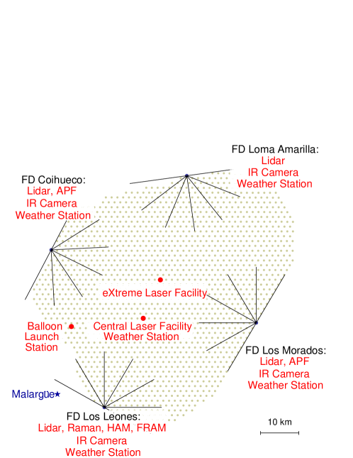
Figure 1: The Surface Detector stations and Fluorescence Detector sites of the Pierre Auger Observatory. Also shown are the locations of Malargüe and the atmospheric monitoring instruments operating at the Observatory (see text for details).

To remove the effect of atmospheric fluctuations that would otherwise impact FD measurements, an extensive atmospheric monitoring program is carried out at the Pierre Auger Observatory. A list of monitors and their locations relative to the FD buildings and SD array are shown in fig. 1. Atmospheric conditions at ground level are measured by a network of weather stations at each FD site and in the center of the SD; these provide updates on ground-level conditions every five minutes. In addition, regular meteorological radiosonde flights (one or two per week) are used to measure the altitude profiles of atmospheric pressure, temperature, and other bulk properties of the air. The weather station monitoring and radiosonde flights are performed day or night, independent of the FD data acquisition.

During the dark periods suitable for FD data-taking, hourly measurements of aerosols are made using the FD telescopes, which record vertical UV laser tracks produced by a Central Laser Facility (CLF) deployed on site since 2003 [20]. These measurements are augmented by data from lidar stations located near each FD building [21], a Raman lidar at one FD site, and the eXtreme Laser Facility (or XLF, named for its remote location) deployed in November 2008. Two Aerosol Phase Function Monitors (APFs) are used to determine the aerosol scattering properties of the atmosphere using collimated horizontal light beams produced by Xenon flashers [22]. Two optical telescopes — the Horizontal Attenuation Monitor (HAM) and the (F/ph)otometric Robotic Telescope for Atmospheric Monitoring (FRAM) — record data used to determine the wavelength dependence of the aerosol attenuation [23, 24]. Finally, clouds are measured hourly by the lidar stations, and infrared cameras on the roof of each FD building are used to record the cloud coverage in the FD field of view every five minutes [25].

3 The Production of Light by the Shower and its Transmission through the Atmosphere

Atmospheric conditions impact on both the production and transmission of UV shower light recorded by the FD. The physical conditions of the molecular atmosphere have several effects on fluorescence light production, which we summarize in Section 3.1. We treat light transmission, outlined in Section 3.2, primarily as a single-scattering process characterized by the atmospheric optical depth (Sections 3.2.1 and 3.2.2) and scattering angular dependence (Section 3.2.3). Multiple scattering corrections to atmospheric transmission are discussed in Section 3.2.4.

3.1 The Effect of Weather on Light Production

The yields of light from the Cherenkov and fluorescence emission processes depend on the physical conditions of the gaseous mixture of molecules in the atmosphere. The production of Cherenkov light is the simpler of the two cases, since the number of photons emitted per charged particle per meter per wavelength interval depends only on the refractive index of the atmosphere $n(\lambda,p,T)$. The dependence of this quantity on pressure, temperature, and wavelength $\lambda$ can be estimated analytically, and so the effect of weather on the light yield from the Cherenkov process are relatively simple to incorporate into air shower reconstructions.

The case of fluorescence light is more complex, not only because it is necessary to consider additional weather effects on the light yield, but also due to the fact that several of these effects can be determined only by difficult experimental measurements (see [26, 27, 28, 29] and references in [30]).

One well-known effect of the weather on light production is the collisional quenching of fluorescence emission, in which the radiative transitions of excited nitrogen molecules are suppressed by molecular collisions. The rate of collisions depends on pressure and temperature, and the form of this dependence can be predicted by kinetic gas theory [1, 27]. However, the cross section for collisions is itself a function of temperature, which introduces an additional term into the $p$ and $T$ dependence of the yield. The temperature dependence of the cross section cannot be predicted a priori, and must be determined with laboratory measurements [31].

Water vapor in the atmosphere also contributes to collisional quenching, and so the fluorescence yield has an additional dependence on the absolute humidity of the atmosphere. This dependence must also be determined experimentally, and its use as a correction in shower reconstructions using the fluorescence technique requires regular measurements of the altitude profile of humidity. A full discussion of these effects is beyond the scope of this paper, but detailed descriptions are available in [2, 10, 32]. We will summarize the estimates of their effect on shower energy and $X_{\text{max}}$ in Section 6.1.

3.2 The Effect of Weather on Light Transmission

The attenuation of light along a path through the atmosphere between a light source and an observer can be expressed as a transmission coefficient $\mathcal{T}$, which gives the fraction of light not absorbed or scattered along the path. If the optical thickness (or optical depth) of the path is $\tau$, then $\mathcal{T}$ is estimated using the Beer-Lambert-Bouguer law:

$$\mathcal{T}=e^{-\tau}.$$ (1)

The optical depth of the air is affected by the density and composition of molecules and aerosols, and can be treated as the sum of molecular and aerosol components: $\tau=\tau_{m}+\tau_{a}$. The optical depth is a function of wavelength and the orientation of a path within the atmosphere. However, if the atmospheric region of interest is composed of horizontally uniform layers, then the full spatial dependence of $\tau$ reduces to an altitude dependence, such that $\tau\equiv\tau(h,\lambda)$. For a slant path elevated at an angle $\varphi$ above the horizon, the light transmission along the path between the ground and height $h$ is

$$\mathcal{T}(h,\lambda,\varphi)=e^{-\tau(h,\lambda)/\sin{\varphi}}.$$ (2)

In an air fluorescence detector, a telescope recording isotropic fluorescence emission of intensity $I_{0}$ from a source of light along a shower track will observe an intensity

$$I=I_{0}\cdot\mathcal{T}_{m}\cdot\mathcal{T}_{a}\cdot(1+H.O.)\cdot\frac{\Delta\Omega}{4\pi}\text{,}$$ (3)

where $\Delta\Omega$ is the solid angle subtended by the telescope diaphragm as seen from the light source. The molecular and aerosol transmission factor $\mathcal{T}_{m}$ $\cdot$$\mathcal{T}_{a}$ primarily represents single-scattering of photons out of the field of view of the telescope. In the ultraviolet range used for air fluorescence measurements, the absorption of light is much less important than scattering [11, 33], although there are some exceptions discussed in Section 3.2.1. The term $H.O.$ is a higher-order correction to the Beer-Lambert-Bouguer law that accounts for the single and multiple scattering of Cherenkov and fluorescence photons into the field of view.

To estimate the transmission factors and scattering corrections needed in eq. (3), it is necessary to measure the vertical height profile and wavelength dependence of the optical depth $\tau(h,\lambda)$, as well as the angular distribution of light scattered from atmospheric particles, also known as the phase function $P(\theta)$. For these quantities, the contributions due to molecules and aerosols are considered separately.

3.2.1 The Optical Depth of Molecules

The probability per unit length that a photon will be scattered or absorbed as it moves through the atmosphere is given by the total volume extinction coefficient

$$\alpha_{\text{ext}}(h,\lambda)=\alpha_{\text{abs}}(h,\lambda)+\beta(h,\lambda)\text{,}$$ (4)

where $\alpha_{\text{abs}}$ and $\beta$ are the coefficients of absorption and scattering, respectively. The vertical optical depth between a telescope at ground level and altitude $h$ is the integral of the atmospheric extinction along the path:

$$\tau(h,\lambda)=\int_{h_{\text{gnd}}}^{h}\alpha_{\text{ext}}(h^{\prime},\lambda)dh^{\prime}.$$ (5)

Molecular extinction in the near UV is primarily an elastic scattering process, since the Rayleigh scattering of light by molecular nitrogen (N₂) and oxygen (O₂) dominates inelastic scattering and absorption [34]. For example, the Raman scattering cross sections of N₂ and O₂ are approximately $10^{-30}$ cm^-2 between $300-420$ nm [35], much smaller than the Rayleigh scattering cross section of air ($\sim 10^{-27}$ cm^-2) at these wavelengths [36]. Moreover, while O₂ is an important absorber in the deep UV, its absorption cross section is effectively zero for wavelengths above $240$ nm [33]. Ozone (O₃) molecules absorb light in the UV and visible bands, but O₃ is mainly concentrated in a high-altitude layer above the atmospheric volume used for air fluorescence measurements [33].

Therefore, for the purpose of air fluorescence detection, the total molecular extinction $\alpha_{\text{ext}}^{m}(h,\lambda)$ simply reduces to the scattering coefficient $\beta_{m}(h,\lambda)$. At standard temperature and pressure, molecular scattering can be defined analytically in terms of the Rayleigh scattering cross section [36, 37]:

$$\beta^{\text{STP}}_{m}(h,\lambda)\equiv\beta_{s}(\lambda)=N_{s}\sigma_{\text{R}}(\lambda)=\frac{24\pi^{3}}{N_{s}\lambda^{4}}\left(\frac{n_{s}^{2}(\lambda)-1}{n_{s}^{2}(\lambda)+2}\right)^{2}\frac{6+3\rho(\lambda)}{6-7\rho(\lambda)}.$$ (6)

In this expression, $N_{s}$ is the molecular number density under standard conditions and $n_{s}(\lambda)$ is the index of refraction of air. The depolarization ratio of air, $\rho(\lambda)$, is determined by the asymmetry of N₂ and O₂ molecules, and its value is approximately $0.03$ in the near UV [36]. The wavelength dependence of these quantities means that between $300$ nm and $420$ nm, the wavelength dependence of molecular scattering shifts from the classical $\lambda^{-4}$ behavior to an effective value of $\lambda^{-4.2}$.

Since the atmosphere is an ideal gas, the altitude dependence of the scattering coefficient can be expressed in terms of the vertical temperature and pressure profiles $T(h)$ and $p(h)$,

$$\alpha_{\text{ext}}^{m}(h,\lambda)\equiv\beta_{m}(h,\lambda)=\beta_{s}(\lambda)\frac{p(h)}{p_{s}}\frac{T_{s}}{T(h)}\text{,}$$ (7)

where $T_{s}$ and $p_{s}$ are standard temperature and pressure [36]. Given the profiles $T(h)$ and $p(h)$ obtained from balloon measurements or local climate models, the vertical molecular optical depth is estimated via numerical integration of equations (5) and (7).

3.2.2 The Optical Depth of Aerosols

The picture is more complex for aerosols than for molecules because in general it is not possible to calculate the total aerosol extinction coefficient analytically. The particulate scattering theory of Mie, for example, depends on the simplifying assumption of spherical scatterers [38], a condition which often does not hold in the field. Moreover, aerosol scattering depends on particle composition, which can change quite rapidly depending on the wind and weather conditions.

Therefore, knowledge of the aerosol transmission factor $\mathcal{T}_{a}$ depends on frequent field measurements of the vertical aerosol optical depth $\tau_{a}(h,\lambda)$. Like other aerosol properties, the altitude profile of $\tau_{a}(h,\lambda)$ can change dramatically during the course of a night. However, in general $\tau_{a}(h,\lambda)$ increases rapidly with $h$ only in the first few kilometers above ground level, due to the presence of mixed aerosols in the planetary boundary layer.

In the lower atmosphere, the majority of aerosols are concentrated in the mixing layer. The thickness of the mixing layer is measured from the prevailing ground level in the region, and its height roughly follows the local terrain (excluding small hills and escarpments). This gives the altitude profile of $\tau_{a}(h,\lambda)$ a characteristic shape: a nearly linear increase at the lowest heights, followed by a flattening as the aerosol density rapidly decreases with altitude. Figure 2 depicts an optical depth profile inferred using vertical laser shots from the CLF at $355$ nm viewed from the FD site at Los Leones. The profile, corresponding to a moderately clear atmosphere, can be considered typical of this location. Also shown is the aerosol transmission coefficient between points along the vertical laser beam and the viewing FD, corresponding to a ground distance of $26$ km.

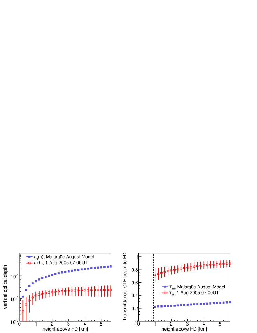
Figure 2: Left: a vertical aerosol optical depth profile $\tau_{a}(h,355~{}\text{nm})$ measured using the FD at Los Leones with vertical laser shots from the CLF ($26$ km distance). The uncertainties are dominated by systematic effects and are highly correlated. Also shown is the monthly average molecular optical depth $\tau_{m}(h,355~{}\text{nm})$. Right: molecular and aerosol light transmission factors for the atmosphere between the vertical CLF laser beam and the Los Leones FD. The dashed line at $1$ km indicates the lower edge of the FD field of view at this distance (see Section 5.1.1 for details).

The wavelength dependence of $\tau_{a}(h,\lambda)$ depends on the wavelength of the incident light and the size of the scattering aerosols. A conventional parameterization for the dependence is a power law due to Ångstrøm [39],

$$\tau_{a}(h,\lambda)=\tau(h,\lambda_{0})\cdot\left(\frac{\lambda_{0}}{\lambda}\right)^{\gamma},$$ (8)

where $\gamma$ is known as the Ångstrøm exponent. The exponent is also measured in the field, and the measurements are normalized to the value of the optical depth at a reference wavelength $\lambda_{0}$. The normalization point used at the Auger Observatory is the wavelength of the Central Laser Facility, $\lambda_{0}=355$ nm, approximately in the center of the nitrogen fluorescence spectrum.

The Ångstrøm exponent is determined by the size distribution of scattering aerosols, such that smaller particles have a larger exponent — eventually reaching the molecular limit of $\gamma\approx 4$ — while larger particles give rise to a smaller $\gamma$ and thus a more “wavelength-neutral” attenuation [40, 41]. For example, in a review of the literature by Eck et al. [42], aerosols emitted from burning vegetation and urban and industrial areas are observed to have a relatively large Ångstrøm coefficient ($\gamma=1.41\pm 0.35$). These environments are dominated by fine ($<1~{}\mu$m) “accumulation mode” particles, or aerodynamically stable aerosols that do not coalesce or settle out of the atmosphere. In desert environments, where coarse ($>1~{}\mu$m) particles dominate, the wavelength dependence is almost negligible [42, 43].

3.2.3 Angular Dependence of Molecular and Aerosol Scattering

Only a small fraction of the photons emitted from an air shower arrive at a fluorescence detector without scattering. The amount of scattering must be estimated during the reconstruction of the shower, and so the scattering properties of the atmosphere need to be well understood.

For both molecules and aerosols, the angular dependence of scattering is described by normalized angular scattering cross sections, which give the probability per unit solid angle $P(\theta)=\sigma^{-1}d\sigma/d\Omega$ that light will scatter out of the beam path through an angle $\theta$. Following the convention of the atmospheric literature, this work will refer to the normalized cross sections as the molecular and aerosol phase functions.

The molecular phase function $P_{m}(\theta)$ can be estimated analytically, with its key feature being the symmetry in the forward and backward directions. It is proportional to the $(1+\cos^{2}{\theta})$ factor of the Rayleigh scattering theory, but in air there is a small correction factor $\delta\approx 1\%$ due to the anisotropy of the N₂ and O₂ molecules [36]:

$$P_{m}(\theta)=\frac{3}{16\pi(1+2\delta)}\left(1+3\delta+(1-\delta)\cos^{2}{\theta}\right).$$ (9)

The aerosol phase function $P_{a}(\theta)$, much like the aerosol optical depth, does not have a general analytical solution, and in fact its behavior as a function of $\theta$ is quite complex. Therefore, one is often limited to characterizing the gross features of the light scattering probability distribution, which is sufficient for the purposes of air fluorescence detection. In general, the angular distribution of light scattered by aerosols is very strongly peaked in the forward direction, reaches a minimum near $90^{\circ}$, and has a small backscattering component. It is reasonably approximated by the parameterization [22, 44, 45]

$$P_{a}(\theta)=\frac{1-g^{2}}{4\pi}\cdot\left(\frac{1}{(1+g^{2}-2g\cos{\theta})^{3/2}}+f\frac{3\cos^{2}{\theta}-1}{2(1+g^{2})^{3/2}}\right).$$ (10)

The first term, a Henyey-Greenstein scattering function [46], corresponds to forward scattering; and the second term — a second-order Legendre polynomial, chosen so that it does not affect the normalization of $P_{a}(\theta)$ — accounts for the peak at large $\theta$ typically found in the angular distribution of aerosol-scattered light. The quantity $g=\langle\cos{\theta}\rangle$ measures the asymmetry of scattering, and $f$ determines the relative strength of the forward and backward scattering peaks. The parameters $f$ and $g$ are observable quantities which depend on local aerosol characteristics.

3.2.4 Corrections for Multiple Scattering

As light propagates from a shower to the FD, molecular and aerosol scattering can remove photons that would otherwise travel along a direct path toward an FD telescope. Likewise, some photons with initial paths outside the detector field of view can be scattered back into the telescope, increasing the apparent intensity and angular width of the shower track.

During the reconstruction of air showers, it is convenient to consider the addition and subtraction of scattered photons to the total light flux in separate stages. The subtraction of light is accounted for in the transmission coefficients $\mathcal{T}_{m}$ and $\mathcal{T}_{a}$ of eq. (3). Given the shower geometry and measurements of atmospheric scattering conditions, the estimation of $\mathcal{T}_{m}$ and $\mathcal{T}_{a}$ is relatively straightforward. However, the addition of light due to atmospheric scattering is less simple to calculate, due to the contributions of multiple scattering. Multiple scattering has no universal analytical description, and those analytical solutions which do exist are only valid under restrictive assumptions that do not apply to typical FD viewing conditions [47].

A large fraction of the flux of photons from air showers recorded by an FD telescope can come from multiply-scattered light, particularly within the first few kilometers above ground level, where the density of scatterers is highest. In poor viewing conditions, $10\%-15\%$ of the photons arriving from the lower portion of a shower track may be due to multiple scattering. Since these contributions cannot be neglected, a number of Monte Carlo studies have been carried out to quantify the multiply-scattered component of recorded shower signals under realistic atmospheric conditions [47, 48, 49, 50]. The various simulations indicate that multiple scattering grows with optical depth and distance from the shower. Based on these results, Roberts [47] and Pekala et al. [50] have developed parameterizations of the fraction of multiply-scattered photons in the shower image. Both parameterizations are implemented in the FD event reconstruction, and their effect on estimates of the shower energy and shower maximum are described in section 6.3.

4 Molecular Measurements at the Pierre Auger Observatory

4.1 Profile Measurements with Weather Stations and Radiosondes

The vertical profiles of atmospheric parameters (pressure, temperature, etc.) vary with geographic location and with time so that a global static model of the atmosphere is not appropriate for precise shower studies. At a given location, the daily variation of the atmospheric profiles can be as large as the variation in the seasonal average conditions. Therefore, daily measurements of atmospheric profiles are desirable.

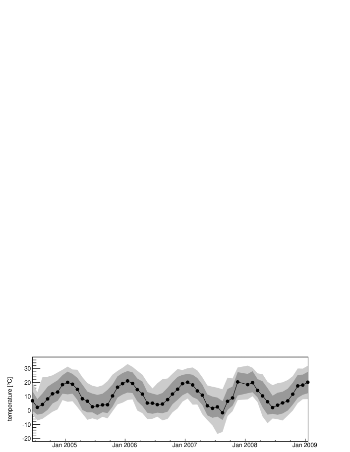
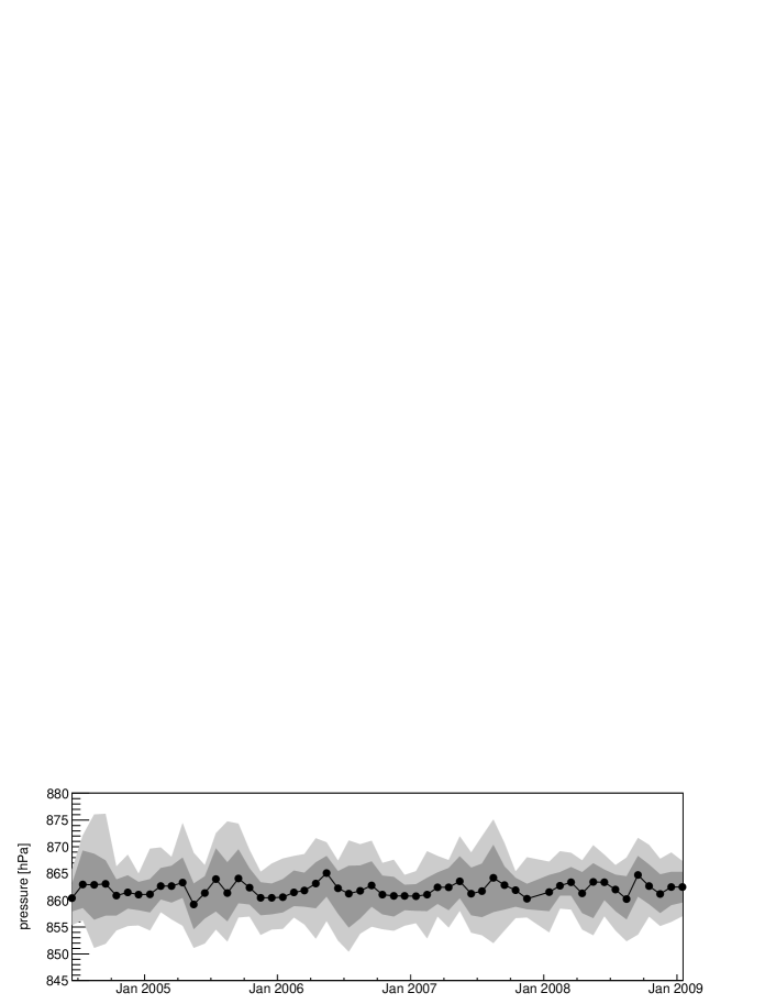
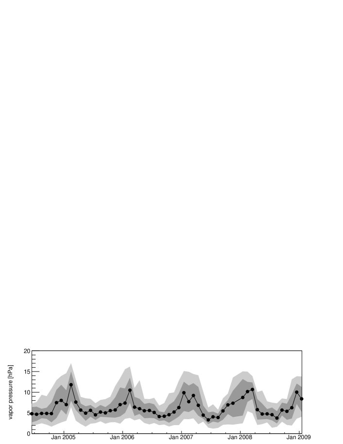
Figure 3: Monthly median ground temperature, pressure, and water vapor pressure observed at the CLF weather station ($1.4$ km above sea level), showing the distributions of 68% and 95% of the measurements as dark and light gray contours, respectively. The vapor pressure has been calculated using measurements of the temperature and relative humidity.

Several measurements of the molecular component of the atmosphere are performed at the Pierre Auger Observatory. Near each FD site and the CLF, ground-based weather stations are used to record the temperature, pressure, relative humidity, and wind speed every five minutes. The first weather station was commissioned at Los Leones in January 2002, followed by stations at the CLF (June 2004), Los Morados (May 2007), and Loma Amarilla (November 2007). The station at Coihueco is installed but not currently operational. Data from the CLF station are shown in fig. 3; the measurements are accurate to $0.2-0.5^{\circ}$C in temperature, $0.2-0.5$ hPa in pressure, and $2\%$ in relative humidity [51]. The pressure and temperature data from the weather stations are used to monitor the weather dependence of the shower signal observed by the SD [52, 53]. They can also be used to characterize the horizontal uniformity of the molecular atmosphere, which is assumed in eq. (2).

Of more direct interest to the FD reconstruction are measurements of the altitude dependence of the pressure and temperature, which can be used in eq. (7) to estimate the vertical molecular optical depth. These measurements are performed with balloon-borne radiosonde flights, which began in mid-2002 and are currently launched one or two times per week. The radiosonde measurements include relative humidity and wind data recorded about every $20$ m up to an average altitude of $25$ km, well above the fiducial volume of the fluorescence detectors. The accuracy of the measurements are approximately $0.2^{\circ}\text{C}$ for temperature, $0.5-1.0$ hPa for pressure, and $5\%$ for relative humidity [54].

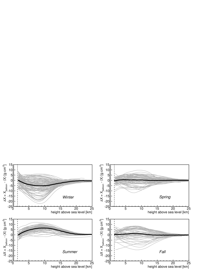
Figure 4: Radiosonde measurements of the depth profile above Malargüe recorded during 261 balloon flights between 2002 and 2009. The data are plotted as deviations from the average profile of all 261 flights, and are grouped by season. The dark lines indicate the seasonal averages, and the vertical dashed lines correspond to the height of Malargüe above sea level.

The balloon observations demonstrate that daily variations in the temperature and pressure profiles depend strongly on the season, with more stable conditions during the austral summer than in winter [7]. The atmospheric depth profile $X(h)$ exhibits significant altitude-dependent fluctuations. The largest daily fluctuations are typically $5$ $\text{g~{}cm}^{-2}$ observed at ground level, increasing to $10-15$ $\text{g~{}cm}^{-2}$ between $6$ and $12$ km altitude. The seasonal differences between summer and winter can be as large as $20$ $\text{g~{}cm}^{-2}$ on the ground, increasing to $30$ $\text{g~{}cm}^{-2}$ at higher altitudes (fig. 4).

4.2 Monthly Average Models

Balloon-borne radiosondes have proven to be a reliable means of measuring the state variables of the atmosphere, but nightly balloon launches are too difficult and expensive to carry out with regularity in Malargüe. Therefore, it is necessary to sacrifice some time resolution in the vertical profile measurements and use models which quantify the average molecular profile over limited time intervals.

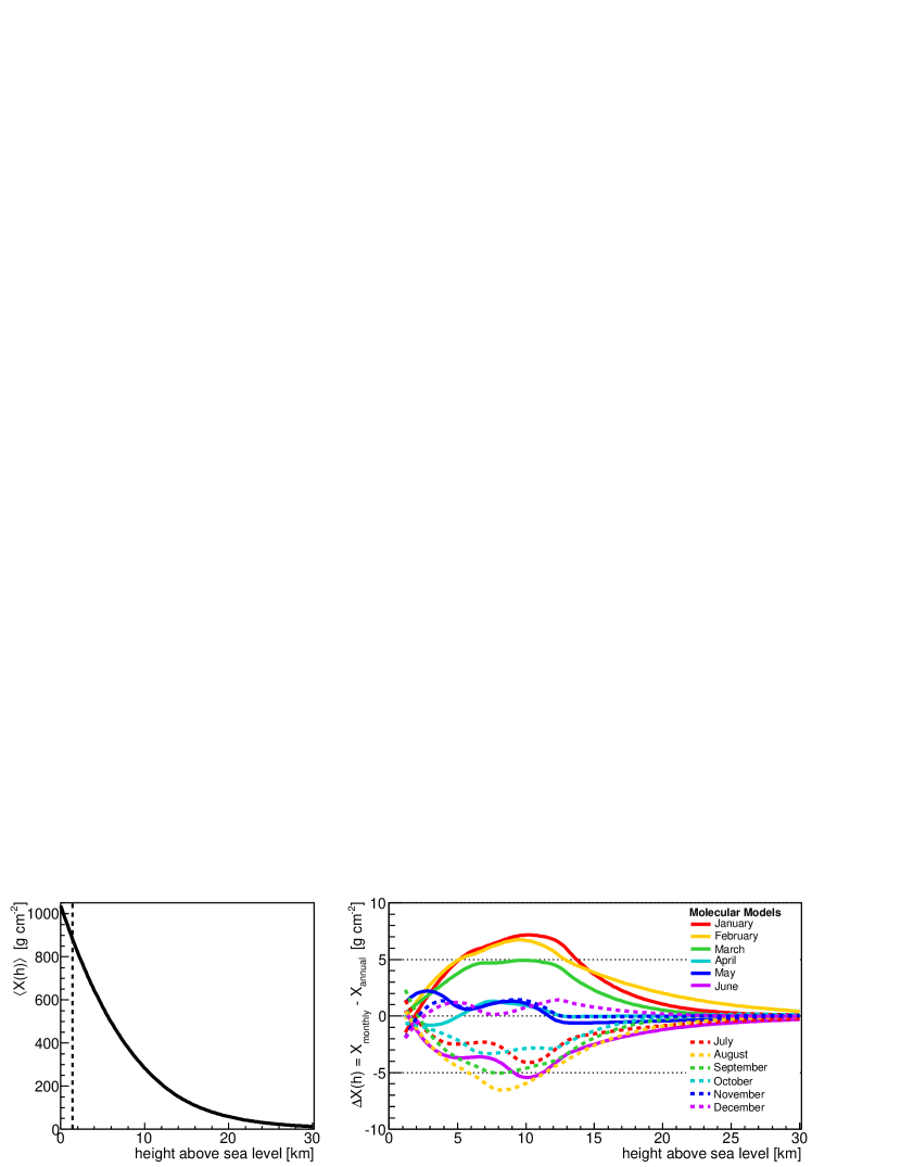
Figure 5: Left: average profile $X(h)$ above Malargüe, with the altitude of the site indicated by the vertical dotted line. Right: deviation of the monthly mean values of $X(h)$ from the yearly average as a function of month. Data are from the mean monthly weather models (updated through 2009).

Such time-averaged models have been generated for the FD reconstruction using $261$ local radiosonde measurements conducted between August 2002 and December 2008. The monthly profiles include average values for the atmospheric depth, density, pressure, temperature, and humidity as a function of altitude. Figure 5 depicts a plot of the annual mean depth profile $X(h)$ in Malargüe, as well as the deviation of the monthly model profiles from the annual average. The uncertainties in the monthly models, not shown in the figure, represent the typical range of conditions observed during the course of each month. At ground level, the RMS uncertainties are approximately $3$ $\text{g~{}cm}^{-2}$ in austral summer and $6$ $\text{g~{}cm}^{-2}$ during austral winter; near $10$ km altitude, the uncertainties are $4$ $\text{g~{}cm}^{-2}$ in austral summer and $8$ $\text{g~{}cm}^{-2}$ in austral winter.

The use of monthly averages rather than daily measurements introduces uncertainties into measurements of shower energies $E$ and shower maxima $X_{\text{max}}$; the magnitudes of the effects are estimated in Section 6.1.

4.3 Horizontal Uniformity of the Molecular Atmosphere

The assumption of horizontally uniform atmospheric layers implied by equation (2) reduces the estimate of atmospheric transmission to a simple geometrical calculation, but the deviation of the atmosphere from true horizontal uniformity introduces some systematic error into the transmission. An estimate of this deviation is required to calculate its impact on air shower reconstruction.

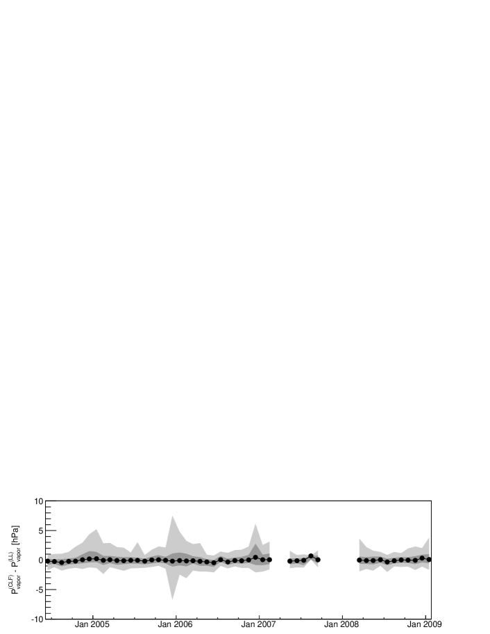
Figure 6: Monthly differences in the ground temperature, pressure, and vapor pressure observed with the weather stations at Los Leones (LL) and the CLF. The dark and light gray contours contain 68% and 95% of the measurement differences. Gaps in the comparison during 2007 were caused by equipment failures in the station at Los Leones.

For the molecular component of the atmosphere, the data from different ground-based weather stations provide a convenient, though limited, check of weather differences across the Observatory. For example, the differences between the temperature, pressure, and vapor pressure measured using the weather stations at Los Leones and the CLF are plotted in fig. 6. The altitude difference between the stations is approximately $10$ m, and they are separated by $26$ km, or roughly half the diameter of the SD. Despite the large horizontal separation of the sites, the measurements are in close agreement. Note that the differences in the vapor pressure are larger than the differences in total pressure, due to the lower accuracy of the relative humidity measurements.

It is quite difficult to check the molecular uniformity at higher altitudes, with, for example, multiple simultaneous balloon launches. The measurements from the network of weather stations at the Observatory are currently the only indications of the long-term uniformity of molecular conditions across the site. Based on these observations, the molecular atmosphere is treated as uniform.

5 Aerosol Measurements at the Pierre Auger Observatory

Several instruments are deployed at the Pierre Auger Observatory to observe aerosol scattering properties. The aerosol optical depth is estimated using UV laser measurements from the CLF, XLF, and scanning lidars (Section 5.1); the aerosol phase function is determined with APF monitors (Section 5.2); and the wavelength dependence of the aerosol optical depth is measured with data recorded by the HAM and FRAM telescopes (Section 5.3).

5.1 Optical Depth Measurements

5.1.1 The Central Laser Facility

The CLF produces calibrated laser “test beams” from its location in the center of the Auger surface detector [20, 55]. Located between $26$ and $39$ km from the FD telescopes, the CLF contains a pulsed $355$ nm laser that fires a depolarized beam in an quarter-hourly sequence of vertical and inclined shots. Light is scattered out of the laser beam, and a small fraction of the scattered light is collected by the FD telescopes. With a nominal energy of $7$ mJ per pulse, the light produced is roughly equal to the amount of fluorescence light generated by a $10^{20}$ eV shower. The CLF-FD geometry is shown in fig. 7.

Figure 7: CLF laser and FD geometry. Vertical shots ($\varphi_{1}=90^{\circ}$) are used for the measurement of $\tau_{a}(h,\lambda_{0})$, with $\lambda_{0}=355$ nm.

The CLF has been in operation since late 2003. Every quarter-hour during FD data acquisition, the laser fires a set of 50 vertical shots. The relative energy of each vertical shot is measured by two “pick-off” energy probes, and the light profiles recorded by the FD telescopes are normalized by the probe measurements to account for shot-by-shot changes in the laser energy. The normalized profiles are then averaged to obtain hourly light flux profiles, in units of photons m^-2 mJ^-1 per 100 ns at the FD entrance aperture [20]. The hourly profiles are determined for each FD site, reflecting the fact that aerosol conditions may not be horizontally uniform across the Observatory during each measurement period.

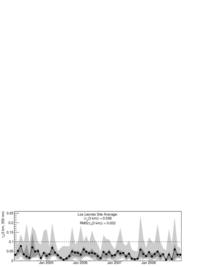
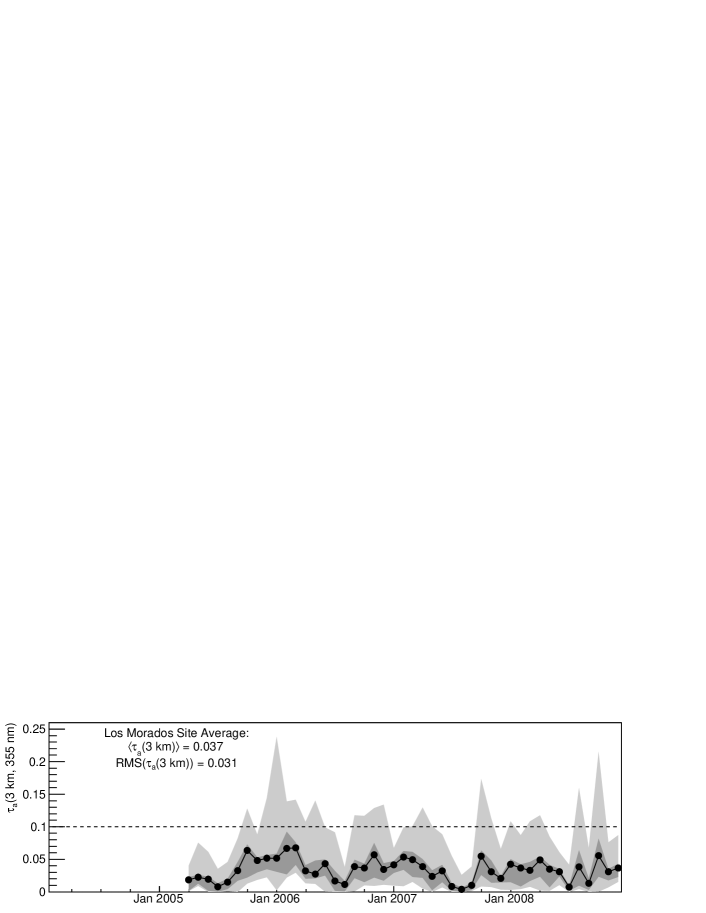
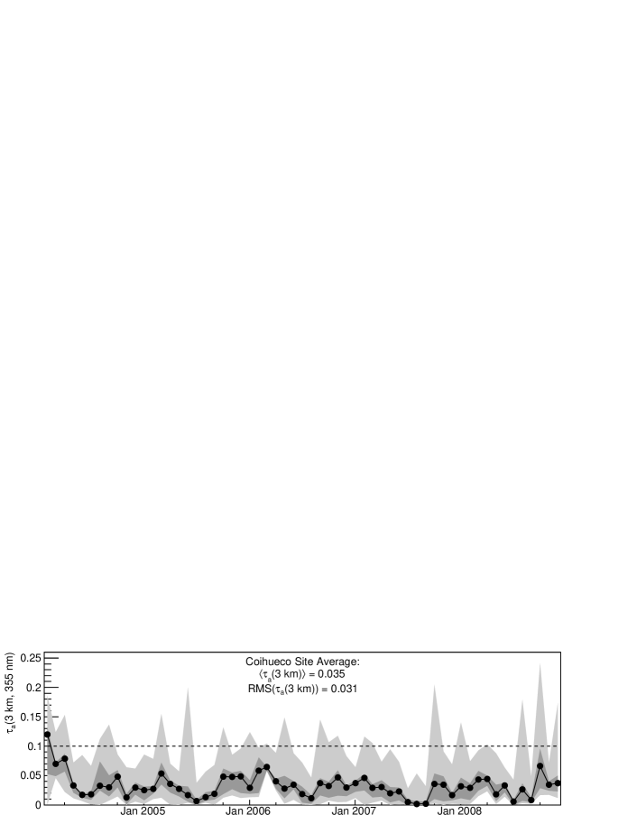
Figure 8: Monthly median CLF measurements of the aerosol optical depth 3 km above the fluorescence telescopes at Los Leones, Los Morados, and Coihueco (January 2004 – December 2008). Measurements from Loma Amarilla are not currently available. The dark and light contours contain 68% and 95% of the measurements, respectively. Hours with optical depths above 0.1 (dashed lines) are characterized by strong haze, and are cut from the FD analysis.

It is possible to determine the vertical aerosol optical depth $\tau_{a}(h,\lambda_{0})$ between the CLF and an FD site by normalizing the observed light flux with a “molecular reference” light profile. The molecular references are simply averaged CLF laser profiles that are observed by the FD telescopes during extremely clear viewing conditions with negligible aerosol attenuation. The references can be identified by the fact that the laser light flux measured by the telescopes during clear nights is larger than the flux on nights with aerosol attenuation (after correction for the relative calibration of the telescopes). Clear-night candidates can also be identified by comparing the shape of the recorded light profile against a laser simulation using only Rayleigh scattering [25]. The candidate nights are then validated by measurements from the APF monitors and lidar stations.

A minimum of three consecutive clear hours are used to construct each reference profile. Once an hourly profile is normalized by a clear-condition reference, the attenuation of the remaining light is due primarily to aerosol scattering along the path from the CLF beam to the telescopes. The optical depth $\tau_{a}(h,\lambda_{0})$ can be extracted from the normalized hourly profiles using the methods described in [56].

Note that the lower elevation limit of the FD telescopes ($1.8^{\circ}$) means that the lowest $1$ km of the vertical laser beam is not within the telescope field of view (see fig. 2). While the CLF can be used to determine the total optical depth between the ground and $1$ km, the vertical distribution of aerosols in the lowest part of the atmosphere cannot be observed. Therefore, the optical depth in this region is constructed using a linear interpolation between ground level, where $\tau_{a}$ is zero, and $\tau_{a}(1~{}\text{km},\lambda_{0})$.

The normalizations used in the determination of $\tau_{a}(h,\lambda_{0})$ mean that the analysis does not depend on the absolute photometric calibration of either the CLF or the FD, but instead on the accuracy of relative calibrations of the laser and the FD telescopes.

The sources of uncertainty that contribute to the normalized hourly profiles include the clear night references ($3\%$), uncertainties in the FD relative calibration ($3\%$), and the accuracy of the laser energy measurement ($3\%$). Statistical fluctuations in the hourly average light profiles contribute additional relative uncertainties of $1\%-3\%$ to the normalized hourly light flux. The uncertainties in $\tau_{a}(h,\lambda_{0})$ plotted in fig. 2 derive from these sources, and are highly correlated due to the systematic uncertainties.

Between January 2004 and December 2008, over 6,000 site-hours of optical depth profiles have been analyzed using measurements of more than one million CLF shots. Figure 8 depicts the distribution of $\tau_{a}(h)$ recorded using the FD telescopes at Los Leones, Los Morados, and Coihueco. The data $3$ km above ground level are shown, since this altitude is typically above the aerosol mixing layer. A moderate seasonal dependence is apparent in the aerosol distributions, with austral summer marked by more haze than winter. The distributions are asymmetric, with long tails extending from the relatively clear conditions ($\tau_{a}(3~{}\text{km})<0.04$) characteristic of most hours to periods of significant haze ($\tau_{a}(3~{}\text{km})>0.1$).

Approximately $5\%$ of CLF measurements have optical depths greater than 0.1. To avoid making very large corrections to the expected light flux from distant showers, these hours are typically not used in the FD analysis.

5.1.2 Lidar Observations

In addition to the CLF, four scanning lidar stations are operated at the Pierre Auger Observatory to record $\tau_{a}(h,\lambda_{0})$ from every FD site [21]. Each station has a steerable frame that holds a pulsed $351$ nm laser, three parabolic mirrors, and three PMTs. The frame is mounted atop a shipping container which contains data acquisition electronics. The station at Los Leones includes a separate, vertically-pointing Raman lidar test system, which can be used to detect aerosols and the relative concentration of N₂ and O₂ in the atmosphere.

During FD data acquisition, the lidar telescopes sweep the sky in a set hourly pattern, pulsing the laser at 333 Hz and observing the backscattered light with the optical receivers. By treating the altitude distribution of aerosols near each lidar station as horizontally uniform, $\tau_{a}(h,\lambda_{0})$ can be estimated from the differences in the backscattered laser signal recorded at different zenith angles [57]. When non-uniformities such as clouds enter the lidar sweep region, the optical depth can still be determined up to the altitude of the non-uniformity.

Since the lidar hardware and measurement techniques are independent of the CLF, the two systems have essentially uncorrelated systematic uncertainties. With the exception of a short hourly burst of horizontal shots toward the CLF and a shoot-the-shower mode (Section 7.2)  [21], the lidar sweeps occur outside the FD field of view to avoid triggering the detector with backscattered laser light. Thus, for many lidar sweeps, the extent to which the lidars and CLF measure similar aerosol profiles depends on the true horizontal uniformity of aerosol conditions at the Observatory.

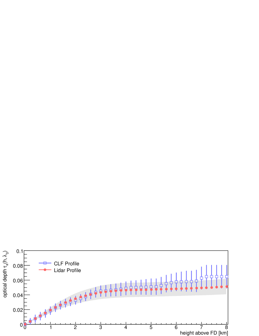
Figure 9: An hourly aerosol optical depth profile observed by the CLF and the Coihueco lidar station for relatively dirty conditions in December 2006. The gray band depicts the systematic uncertainty in the lidar aerosol profile.

Figure 9 shows a lidar measurement of $\tau_{a}(h,\lambda_{0})$ with vertical shots and the corresponding CLF aerosol profile during a period of relatively high uniformity and low atmospheric clarity. The two measurements are in good agreement up to $5$ km, in the region where aerosol attenuation has the greatest impact on FD observations. Despite the large differences in the operation, analysis, and viewing regions of the lidar and CLF, the optical measurements from the two instruments typically agree within their respective uncertainties [23].

5.1.3 Aerosol Optical Depth Uniformity

The FD building at Los Leones is located at an altitude of $1420$ m, on a hill about $15$ m above the surrounding plain, while the Coihueco site is on a ridge at altitude $1690$ m, a few hundred meters above the valley floor. Since the distribution of aerosols follows the prevailing ground level rather than local irregularities, it is reasonable to expect that the aerosol optical depth between Coihueco and a fixed altitude will be systematically lower than the aerosol optical depth between Los Leones and the same altitude. The data in fig. 10 (left panel) support this expectation, and show that aerosol conditions differ significantly and systematically between these FD sites. In contrast, optical depths measured at nearly equal altitudes, such as Los Leones and Los Morados (1420 m), are quite similar.

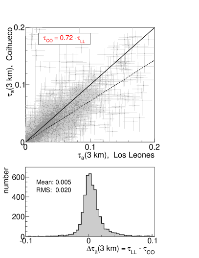
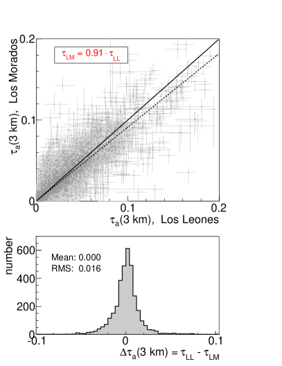
Figure 10: Comparison of the aerosol optical depths measured with CLF shots at Los Leones, Los Morados, and Coihueco. The buildings at Los Leones and Los Morados are located on low hills at similar altitudes, while the Coihueco FD building is on a large hill $200$ m above the other sites. The solid lines indicate equal optical depths at two sites, while the dotted lines show the best linear fits to the optical depths. The bottom panels show histograms of the differences between the optical depths.

Unlike for the molecular atmosphere, it is not possible to assume a horizontally uniform distribution of aerosols across the Observatory. To handle the non-uniformity of aerosols between sites, the FD reconstruction divides the array into aerosol “zones” centered on the midpoints between the FD buildings and the CLF. Within each zone, the vertical distribution of aerosols is treated as horizontally uniform by the reconstruction (i.e., eq. (2) is applied).

5.2 Scattering Measurements

Aerosol scattering is described by the phase function $P_{a}(\theta)$, and the hybrid reconstruction uses the functional form given in equation (10). As explained in Section 3.2.3, the aerosol phase function for each hour must be determined with direct measurements of scattering in the atmosphere, which can be used to infer the backscattering and asymmetry parameters $f$ and $g$ of $P_{a}(\theta)$.

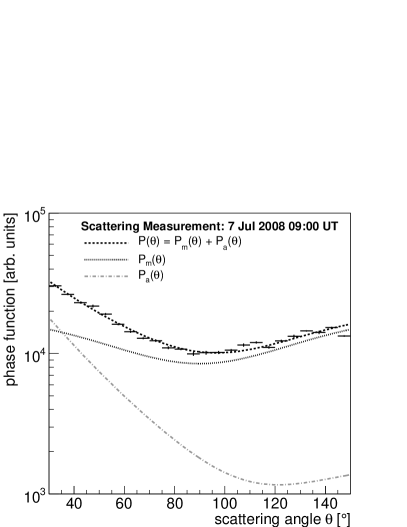
Figure 11: Light scattering measurements with the APF Xenon flasher at Coihueco. During a clear night (left), the observed phase function is symmetric due to the predominance of molecular scattering. An asymmetric phase function on a different night (right) indicates the presence of aerosols.

At the Auger Observatory, these quantities are measured by two Aerosol Phase Function monitors, or APFs, located about $1$ km from the FD buildings at Coihueco and Los Morados [22]. Each APF uses a collimated Xenon flash lamp to fire an hourly sequence of $350$ nm and $390$ nm shots horizontally across the FD field of view. The shots are recorded during FD data acquisition, and provide a measurement of scattering at angles between $30^{\circ}$ and $150^{\circ}$. A fit to the horizontal track seen by the FD is sufficient to determine $f$ and $g$. The APF light signal from two different nights is depicted in fig. 11, showing the total phase function fit and $P_{a}(\theta)$ after the molecular component has been subtracted.

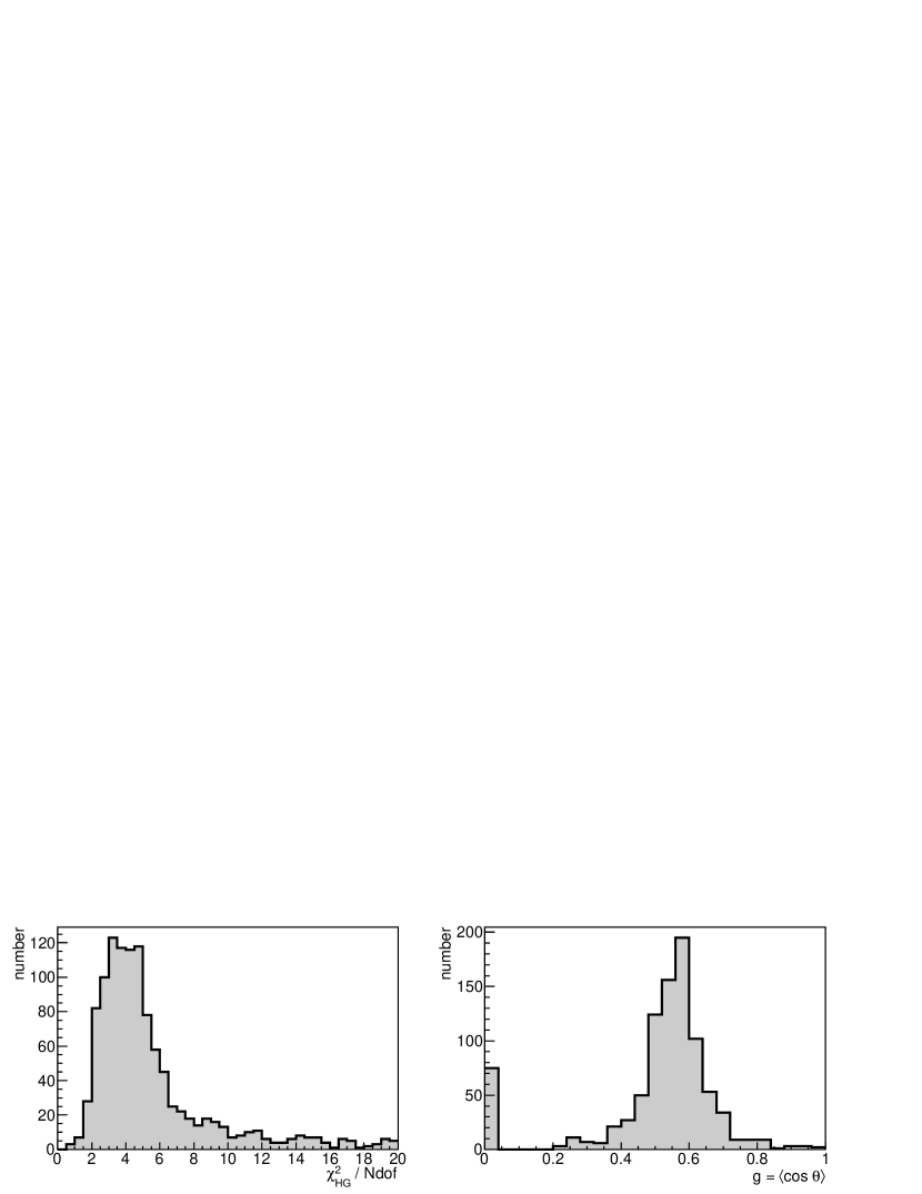
Figure 12: Left: distribution of the figure of merit for fits of equation (10) to APF measurements at Coihueco, June 2006 – July 2008. Right: distribution of the asymmetry parameter $g$ measured at $350$ nm and $390$ nm at Coihueco.

The phase function asymmetry parameter $g$ measured at Coihueco between June 2006 and July 2008 is shown in fig. 12. The value of $g$ was determined by fitting the modified Henyey-Greenstein function of eq. (10) to the APF data. The reduced-$\chi^{2}$ distribution for this fit, also shown in the figure, indicates that the Henyey-Greenstein function describes aerosol scattering in the FD reasonably well. The measurements at Coihueco yield a site average $\langle g\rangle=0.56\pm 0.10$ for the local asymmetry parameter, excluding clear nights without aerosol attenuation. On clear (or nearly clear) nights, we estimate $g=0$ with an uncertainty of $0.2$. The distribution of $g$ in Malargüe, a desert location with significant levels of sand and volcanic dust, is comparable to measurements reported in the literature for similar climates [58].

Approximately 900 hours of phase function data have been recorded with both APF monitors since June 2006. The sparse data mean that it is not possible to use a true measurement of $P_{a}(\theta)$ for most FD events. Therefore, the Coihueco site average is currently used as the estimate of the phase function for all aerosol zones, for all cosmic ray events. The systematic uncertainty introduced by this assumption will be explored in Section 6.2.3.

5.3 Wavelength Dependence

Measurements of the wavelength dependence of aerosol transmission are used to determine the Ångstrøm exponent $\gamma$ defined in equation (8). At the Pierre Auger Observatory, observations of $\gamma$ are performed by two instruments: the Horizontal Attenuation Monitor, or HAM; and the (F/ph)otometric Robotic Telescope for Astronomical Monitoring, also known as FRAM [23, 24].

The HAM uses a high intensity discharge lamp located at Coihueco to provide an intense broad band light source for a CCD camera placed at Los Leones, about $45$ km distant. This configuration allows the HAM to measure the total horizontal atmospheric attenuation across the Observatory. To determine the wavelength dependence of the attenuation, the camera uses a filter wheel to record the source image at five wavelengths between $350$ and $550$ nm. By fitting the observed intensity as a function of wavelength, subtracting the estimated molecular attenuation, and assuming an aerosol dependence of the form of equation (8), it is possible to determine the Ångstrøm exponent $\gamma$ of aerosol attenuation. During 2006 and 2007, the average exponent observed by the HAM was $\gamma=0.7$ with an RMS of $0.5$ due to the non-Gaussian distribution of measurements [23]. The relatively small value of $\gamma$ suggests that Malargüe has a large component of coarse-mode aerosols. This is consistent with physical expectations and other measurements in desert-like environments [42, 59].

Like the APF monitor data, the HAM and FRAM results are too sparse to use in the full reconstruction; therefore, during the FD reconstruction, the HAM site average for $\gamma$ is applied to all FD events in every aerosol zone. The result of this approximation is described in the next section.

6 Impact of the Atmosphere on Accuracy of Reconstruction of Air Shower Parameters

The atmospheric measurements described in Sections 4 and 5 are fully integrated into the software used to reconstruct hybrid events [60]. The data are stored in multi-gigabyte MySQL databases and indexed by observation time, so that the atmospheric conditions corresponding to a given event are automatically retrieved during off-line reconstruction. The software is driven by XML datacards that provide “switches” to study different effects on the reconstruction [60]: for example, aerosol attenuation, multiple scattering, water vapor quenching, and other effects can be switched on or off while reconstructing shower profiles. Propagation of atmospheric uncertainties is also available.

In this section, we estimate the influence of atmospheric effects and the uncertainties in our knowledge of these effects on the reconstruction of hybrid events recorded between December 2004 and December 2008. The data have been subjected to strong quality cuts to remove events contaminated with clouds, as well as geometry cuts to eliminate events poorly viewed by the FD telescopes. These cuts include:

• Gaisser-Hillas fit of the shower profile with $\chi^{2}/\text{NDF}<2.5$

• Gaps in the recorded light profile $<20\%$ of the length of the profile

• Shower maximum $X_{\text{max}}$ observed within the field of view of the FD telescopes

• Uncertainty in $X_{\text{max}}$ (before atmospheric corrections) $<40$ $\text{g~{}cm}^{-2}$

• Relative uncertainty in energy (before atmospheric corrections) $<20\%$

The cuts are the same as those used in studies of the energy spectrum [61, 62] and $X_{\text{max}}$ distribution [63]. We first describe the effects of the molecular information on the determinations of energy and $X_{\text{max}}$. This is followed by a discussion of the impact of aerosol information on the measurement of these quantities.

6.1 Systematic Uncertainties due to the Molecular Atmosphere

6.1.1 Monthly Models

The molecular transmission is determined largely by atmospheric pressure and temperature, as described in eq. (7). For the purpose of reconstruction, these quantities are described by monthly molecular models generated using local radiosonde data. Pressure and temperature also affect the fluorescence yield via collisional quenching, and this effect is included in the hybrid reconstruction.

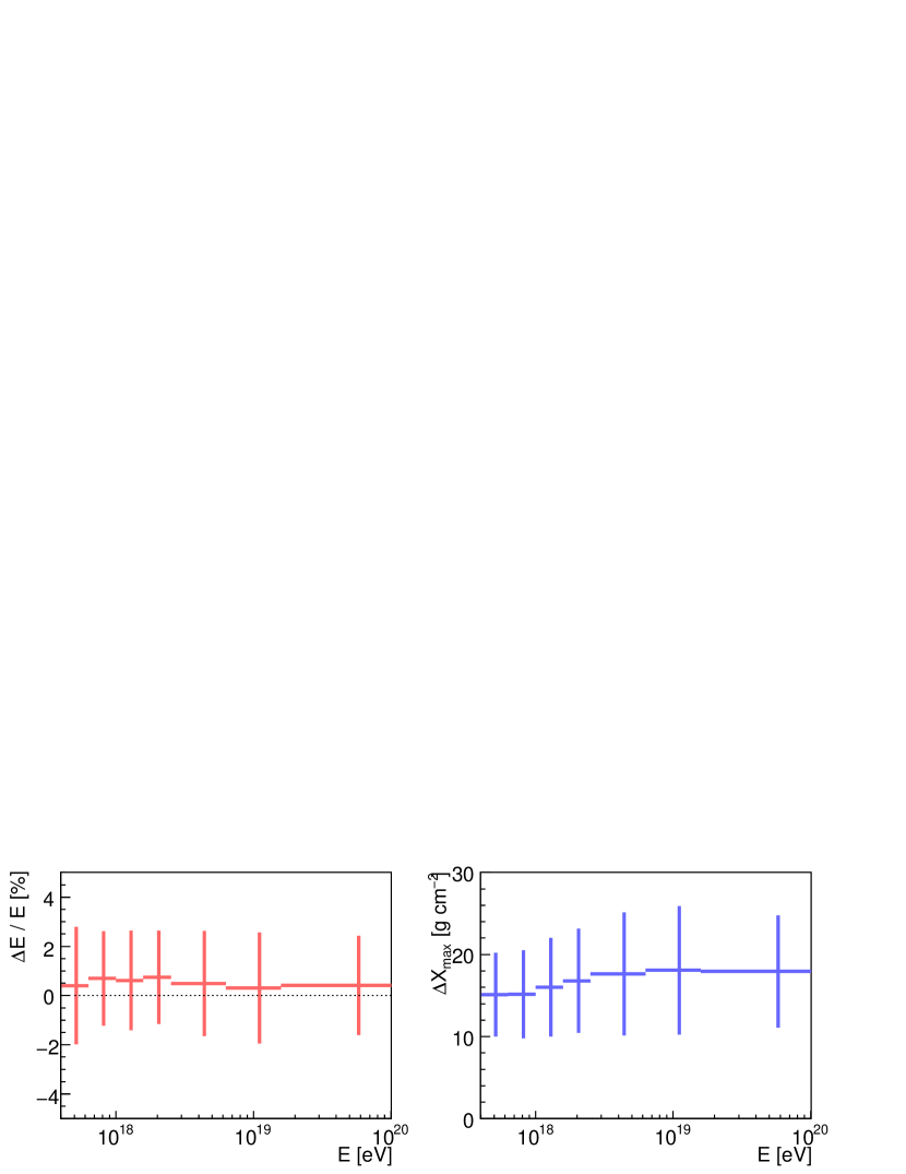
Figure 13: Comparison of hybrid events reconstructed using monthly balloon flights vs. the U.S. Standard Atmosphere (1976) profile model [64]. Uncertainties denote the RMS spread.

The importance of local atmospheric profile measurements is illustrated in fig. 13. The hybrid data have been reconstructed using the monthly profile models described in Section 4.2 and compared to events reconstructed with the U.S. Standard Atmosphere [64]. The values of $X_{\text{max}}$ determined using the molecular atmosphere described by the local monthly models are, on average, $15$ $\text{g~{}cm}^{-2}$ larger than the values obtained if the U.S. Standard Atmosphere is used. This shift is energy-dependent because the average distance between shower tracks and the FD telescopes increases with energy. It is clear that the U.S. Standard Atmosphere is not an appropriate climate model for Malargüe; but even a local annual model would introduce seasonal shifts into the measurement of $X_{\text{max}}$ given the monthly variations observed in the local vertical depth profile (fig. 5).

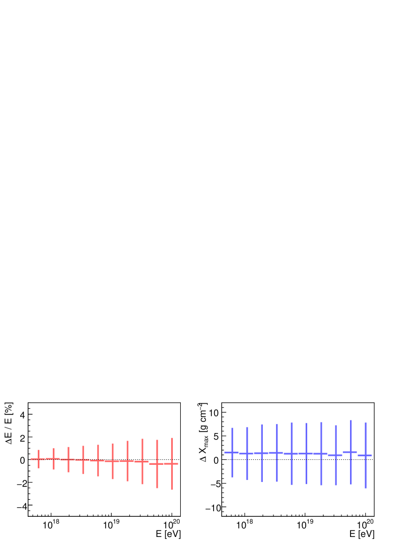
Figure 14: Comparison of simulated events reconstructed with monthly average atmospheric profiles vs. profile measurements from 109 cloud-free balloon flights. The dotted lines indicate the reference for the 109 balloon flights; the uncertainties indicate the RMS spread.

When the monthly models are used, some systematic uncertainties are introduced into the reconstruction due to atmospheric variations that occur on timescales shorter than one month. To investigate this effect, we compare events reconstructed with monthly models vs. local radio soundings. A set of 109 cloud-free, night-time balloon profiles was identified using the cloud camera database. The small number of soundings requires the use of simulated events, so we simulated an equal number of proton and iron showers between $10^{17.5}$ eV and $10^{20}$ eV, reconstructed them with monthly and radiosonde profiles, and applied standard cuts to the simulated dataset. The radiosonde profiles were weighted in the simulation to account for seasonal biases in the balloon launch rate.

The difference between monthly models and balloon measurements is indicated in fig. 14. The use of the models introduces rather small shifts into the reconstructed energy and $X_{\text{max}}$, though there is an energy-dependent increase in the RMS of the measured energies from $0.8\%$ to $2.0\%$ over the simulated energy range. The systematic shift in $X_{\text{max}}$ is about $2$ $\text{g~{}cm}^{-2}$ over the full energy scale, with an RMS of about $8$ $\text{g~{}cm}^{-2}$. We interpret the RMS spread as the decrease in the resolution of the hybrid detector due to variations in the atmospheric conditions within each month.

6.1.2 Combined Effects of Quenching and Atmospheric Variability

The simulations described in Section 6.1.1 used an air fluorescence model that does not correct the fluorescence emission for weather-dependent quenching. Recent estimates of quenching due to water vapor [65, 66] and the $T$-dependence of the N₂-N₂ and N₂-O₂ collisional cross sections [32] allow for detailed studies of their effect on the production of fluorescence light.

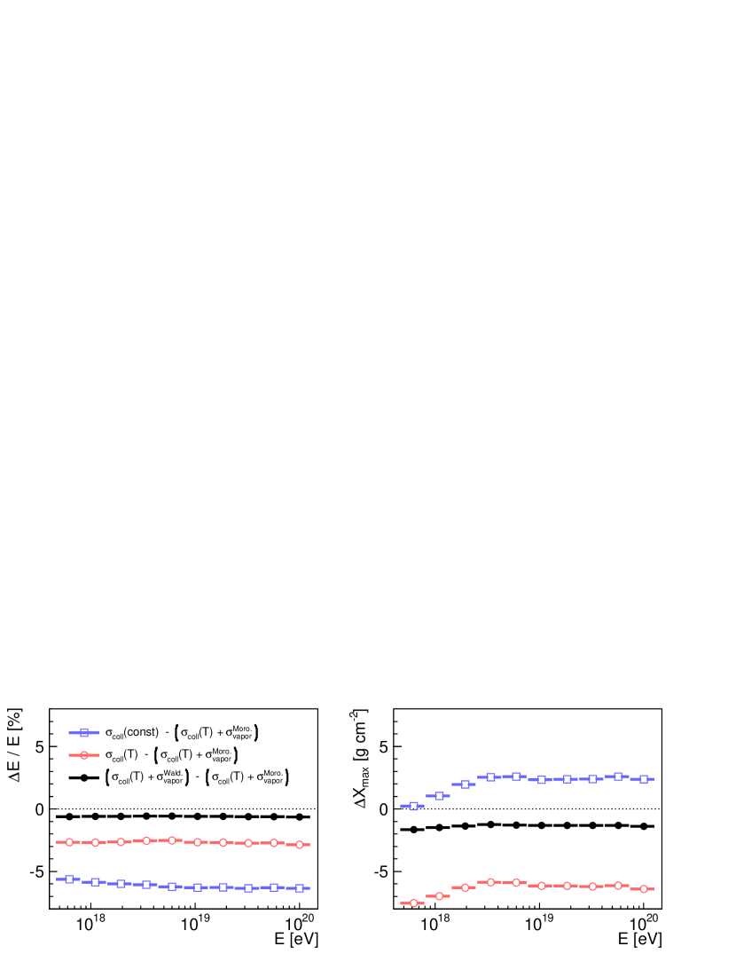
Figure 15: The effect of water vapor quenching and the $T$-dependent N₂-N₂ and N₂-O₂ collisional cross sections $\sigma_{\text{coll}}(T)$ on the reconstructed energy and $X_{\text{max}}$ of simulated showers. The reference (dotted line) corresponds to showers reconstructed with the fluorescence model of Keilhauer et al. [32], which includes $T$-dependent cross sections, and the vapor quenching model of Morozov et al. $(\sigma^{\text{Moro.}}_{\text{vapor}})$ [65]. The markers correspond to different combinations of quenching effects and vapor quenching models. See the text for a detailed explanation.

We have applied the two quenching effects to simulated showers in various combinations using $p$, $T$, and $u$ from the monthly model profiles (see fig. 15). As different quenching effects and models were “switched on” in the reconstruction, the showers were compared to a reference reconstruction that used $T$-dependent collisional cross sections and the vapor quenching model of Morozov et al. [65]. We have considered the following three cases:

1. In the first case, all quenching corrections were omitted (open blue squares in fig. 15). The result is a $5.5\%$ underestimate in shower energy and a $2$ $\text{g~{}cm}^{-2}$ overestimate in $X_{\text{max}}$ with respect to the reference model.

2. In the second case, temperature corrections to the collisional cross section were included, but water vapor quenching was not (open red circles in the figure). Without vapor quenching, the energy is systematically underestimated by $3\%$, and $X_{\text{max}}$ is underestimated by $6-7$ $\text{g~{}cm}^{-2}$ with respect to the reference model.

3. In the third case, all corrections were included, but the vapor quenching model of Waldenmaier et al. [66] was used (closed black circles). The resulting systematic differences are $\Delta E/E$ $=0.5\%$ and $\Delta X_{\text{max}}$ =$2$ $\text{g~{}cm}^{-2}$.

We observe that once water vapor quenching is applied, the particular choice of quenching model has a minor influence. In addition, there is a small total shift in $X_{\text{max}}$ due to the offsetting effects of the $T$-dependent cross sections, which are important at high altitudes, and the effect of water vapor, which is important at low altitudes. The compensation of these two effects leaves the longitudinal profiles of showers relatively undistorted.

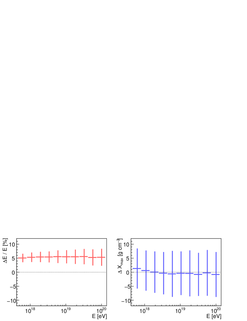
Figure 16: Comparison of simulated events to determine the combined effects of atmospheric variability and quenching corrections. The data were reconstructed in two sets: using monthly profiles plus a fluorescence model without quenching corrections [31]; and using local radiosonde profiles plus a fluorescence model with water vapor quenching and $T$-dependent collisional cross sections [32].

In fig. 16, we plot the combined effects of atmospheric variability around the monthly averages and the quenching corrections. Simulated showers were reconstructed with two settings: monthly average profile models and no quenching corrections; and cloud-free radiosonde profiles with water vapor quenching and $T$-dependent collisional cross sections. The reconstructed energy is increased by $5\%$, on average, and, comparing figs. 14 and 16, we see that the quenching corrections are dominating systematic uncertainties due to the use of monthly models. For $X_{\text{max}}$, the systematic effects of the monthly models offset the quenching corrections. The spread of the combined measurements increases with energy, such that the RMS in energy increases from $1.5\%-3.0\%$, and the RMS in $X_{\text{max}}$ increases from $7.2-8.4$ $\text{g~{}cm}^{-2}$.

6.2 Uncertainties due to Aerosols

For a complete understanding of the effects of aerosols on the reconstruction, several investigations are of interest:

1. A test of the effect of aerosols on the reconstruction, compared to the use of a pure molecular atmosphere.

2. A test of the use of aerosol measurements, compared to a simple parameterization of average aerosol conditions.

3. The propagation of measurement uncertainties in $\tau_{a}(h)$, $\gamma$, $f$, and $g$ in the FD reconstruction, and in particular their effect on uncertainties in energy and $X_{\text{max}}$.

4. A test of the horizontal uniformity of aerosol layers within a zone.

6.2.1 The Comparison of Aerosol Measurements with a Pure Molecular Atmosphere

We have compared the reconstruction of hybrid showers using hourly on-site aerosol measurements with the same showers reconstructed using a purely molecular atmosphere (fig. 17). Neglecting the presence of aerosols causes an $8\%$ underestimate in energy at the lower energies. This underestimate increases to $25\%$ at the higher energies. Moreover, the distribution of shifted energies contains a long tail: $20\%$ of all showers have an energy correction $>20\%$; $7\%$ of showers are corrected by $>30\%$; and $3\%$ of showers are corrected by $>40\%$. The systematic shift in $X_{\text{max}}$ ranges from $-1$ $\text{g~{}cm}^{-2}$ at low energies to almost $10$ $\text{g~{}cm}^{-2}$ at high energies, with an RMS of $10-15$ $\text{g~{}cm}^{-2}$.

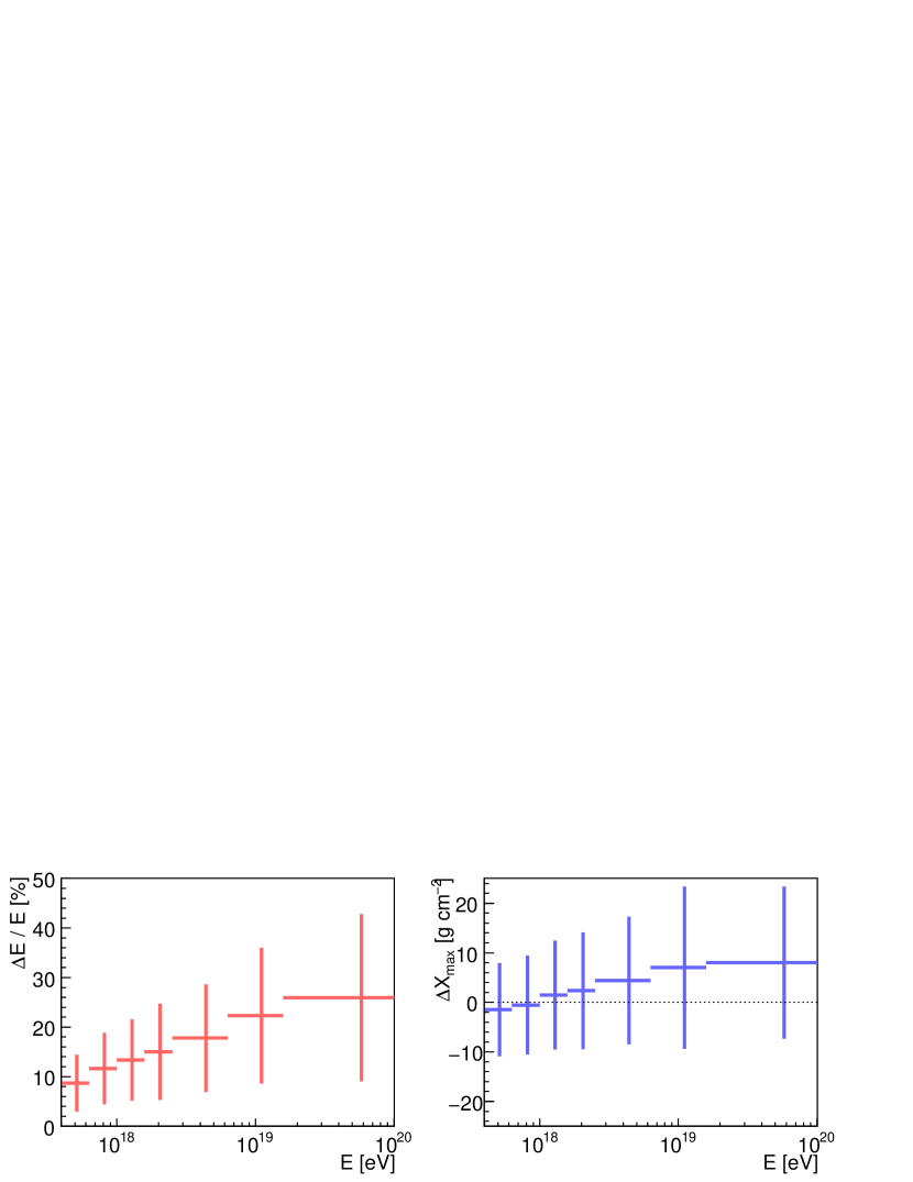
Figure 17: Comparison of hybrid events reconstructed with hourly CLF aerosol measurements vs. no aerosol correction (i.e., purely molecular transmission). Uncertainties indicate the RMS spread for each energy.

6.2.2 The Comparison of Aerosol Measurements with an Average Parameterization

Aerosols clearly play an important role in the transmission and scattering of fluorescence light, but it is natural to ask if hourly measurements of aerosol conditions are necessary, or if a fixed average aerosol parameterization is sufficient for air shower reconstruction.

We can test the sufficiency of average aerosol models by comparing the reconstruction of hybrid events using hourly weather data against the reconstruction using an average profile of the aerosol optical depth in Malargüe. The average profile was constructed using CLF data, and the differences in the reconstruction between this average model and the hourly data are shown in fig. 18, where $\Delta E/E$ and $\Delta X_{\text{max}}$ are grouped by season.

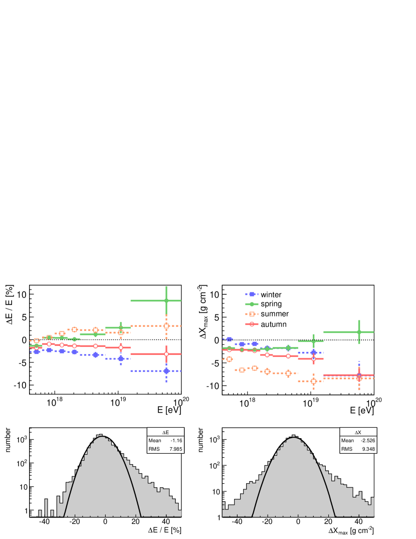
Figure 18: Top: systematic shifts in the hybrid reconstruction of shower energy and $X_{\text{max}}$ caused by the use of average aerosol conditions rather than hourly measurements (indicated by dotted lines). The mean $\Delta E/E$ and $\Delta X_{\text{max}}$ per energy bin, plotted with uncertainties on the means, are arranged by their occurrence in austral winter, spring, summer, and autumn. Bottom: distributions of the differences in energy and $X_{\text{max}}$, shown with Gaussian fits.

Due to the relatively good viewing conditions in Malargüe during austral winter and fall, and poorer atmospheric clarity during the spring and summer, the shifts caused by the use of an average aerosol profile exhibit a strong seasonal dependence. The shifts also exhibit large tails and are energy-dependent. For example, $\Delta E/E$ nearly doubles during the fall, winter, and spring, reaching $-7\%$ (with an RMS of $15\%$) during the winter. The range of seasonal mean offsets in $X_{\text{max}}$ is $+2$ $\text{g~{}cm}^{-2}$ to $-8$ $\text{g~{}cm}^{-2}$ (with an RMS of $15$ $\text{g~{}cm}^{-2}$), and the offsets depend strongly on the shower energy.

6.2.3 Propagation of Uncertainties in Aerosol Measurements

Uncertainties in aerosol properties will cause over- or under-corrections of recorded shower light profiles, particularly at low altitudes and low elevation angles. On average, systematic overestimates of the aerosol optical depth will lead to an over-correction of scattering losses and an overestimate of the shower light flux from low altitudes; this will increase the shower energy estimate and push the reconstructed $X_{\text{max}}$ deeper into the atmosphere. Systematic underestimates of the aerosol optical depth should have the opposite effect.

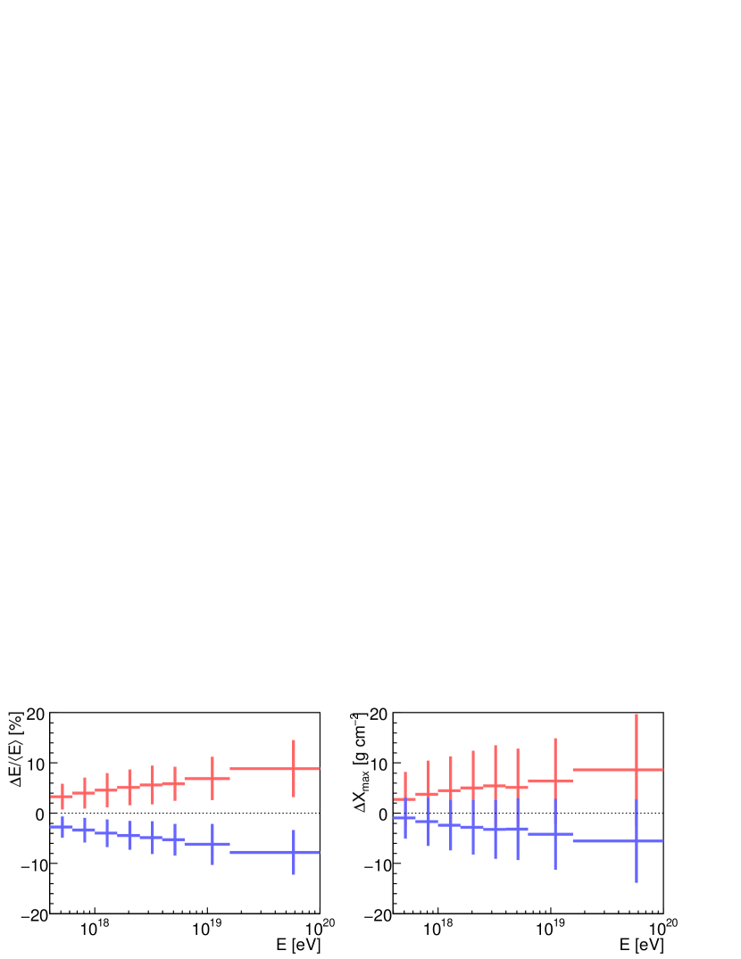
Figure 19: Shifts in the reconstruction of energy and $X_{\text{max}}$ when the aerosol optical depth is varied by its $+1\sigma$ systematic uncertainty (red points) and $-1\sigma$ systematic uncertainty (blue points). The dotted line corresponds to the central aerosol optical depth measurement. The uncertainty bars correspond to the sample RMS in each energy bin.

The primary source of uncertainty in aerosol transmission comes from the aerosol optical depth [67] estimated using vertical CLF laser shots. The uncertainties in the hourly CLF optical depth profiles are dominated by systematic detector and calibration effects, and smoothing of the profiles makes the optical depths at different altitudes highly correlated. Therefore, a reasonable estimate of the systematic uncertainty in energy and $X_{\text{max}}$ can be obtained by shifting the full optical depth profiles by their uncertainties and estimating the mean change in the reconstructed energy and $X_{\text{max}}$.

This procedure was done using hybrid events recorded by telescopes at Los Leones, Los Morados, and Coihueco, and results are shown in fig. 19. The energy dependence of the uncertainties mainly arises from the distribution of showers with distance: low-energy showers tend to be observed during clear viewing conditions and within $10$ km of the FD buildings, reducing the effect of the transmission uncertainties on the reconstruction; and high-energy showers can be observed in most aerosol conditions (up to a reasonable limit) and are observed at larger distances from the FD. The slight asymmetry in the shifts is due to the asymmetric uncertainties of the optical depth profiles.

By contrast to the corrections for the optical depth of the aerosols, the uncertainties that arise from the wavelength dependence of the aerosol scattering and of the phase function are relatively unimportant for the systematic uncertainties in shower energy and $X_{\text{max}}$. By reconstructing showers with average values of the Ångstrøm coefficient and the phase function measured at the Observatory, and comparing the results to showers reconstructed with the $\pm 1~{}\sigma$ uncertainties in these measurements, we find that the wavelength dependence and phase function contribute $0.5\%$ and $1\%$, respectively, to the uncertainty in the energy, and $\sim 2$ $\text{g~{}cm}^{-2}$ to the systematic uncertainty in $X_{\text{max}}$ [67]. Moreover, the uncertainties are largely independent of shower energy and distance.

6.2.4 Evaluation of the Horizontal Uniformity of the Atmosphere

The non-uniformity of the molecular atmosphere, discussed in Section 4.3, is very minor and introduces uncertainties $<1\%$ in shower energies and about $1$ $\text{g~{}cm}^{-2}$ in $X_{\text{max}}$. Non-uniformities in the horizontal distribution of aerosols may also be present, and we expect these to have an effect on the reconstruction. For each FD building, the vertical CLF laser tracks only probe the atmosphere along one light path, but the reconstruction must use this single aerosol profile across the azimuth range observed at each site. In general, the assumption of uniformity within an aerosol zone is reasonable, though the presence of local inhomogeneities such as clouds, fog banks, and sources of dust and smoke may render it invalid.

The assumption of uniformity can be partially tested by comparing data reconstructed with different aerosol zones around each eye: for example, reconstructing showers observed at Los Leones using aerosol data from the Los Leones and Los Morados zones.

Figure 20: Shifts in the estimated shower energy and $X_{\text{max}}$ when data from the FD buildings at Los Morados and Los Leones (dotted line) are reconstructed with swapped aerosol zones. The values give an approximate estimate of the systematic uncertainty due to aerosol non-uniformities across the detector. The uncertainties correspond to the sample RMS in each energy bin.

Data from Los Leones and Los Morados were reconstructed using aerosol profiles from both zones, and the resulting profiles are compared in fig. 20. The mean shifts $\Delta E/E$ and $\Delta X_{\text{max}}$ are relatively constant with energy: $\Delta E/E$ $=0.5\%$, and $\Delta X_{\text{max}}$ is close to zero. The distributions of $\Delta E/E$ and $\Delta X_{\text{max}}$ are affected by long tails, with the RMS in $\Delta E/E$ growing with energy from $3\%$ to $8\%$. For $\Delta X_{\text{max}}$, the RMS for all energies is about 6 $\text{g~{}cm}^{-2}$.

6.3 Corrections for Multiple Scattering

Multiply-scattered light, if not accounted for in the reconstruction, will lead to a systematic overestimate of shower energy and $X_{\text{max}}$. This is because multiple scattering shifts light into the FD field of view that would otherwise remain outside the shower image. A naïve reconstruction will incorrectly identify multiply-scattered photons as components of the direct fluorescence/Cherenkov and singly-scattered Cherenkov signals, leading to an overestimate of the Cherenkov-fluorescence light production used in the calculation of the shower profile. The mis-reconstruction of $X_{\text{max}}$ is similar to what occurs in the case of overestimated optical depths: not enough scattered light is removed from the low-altitude tail of the shower profile, causing an overestimate of $dE/dX$ in the deep part of the profile.

The parameterizations of multiple scattering due to Roberts [47] and Pekala et al. [50] have been implemented in the hybrid event reconstruction. The predictions from both analyses are that the scattered light fraction in the shower image will increase with optical depth, so that distant high-energy showers will be most affected by multiple scattering. A comparison of showers reconstructed with and without multiple scattering (fig. 21) verifies that the shift in the estimated energy doubles from $2\%$ to nearly $5\%$ as the shower energy (and therefore, average shower distance to the FD) increases. The systematic error in the shower maximum is also consistent with the overestimate of the light signal that occurs without multiple scattering corrections.

The multiple scattering corrections due to Roberts and Pekala et al. give rise to small differences in the reconstructed energy and $X_{\text{max}}$. As shown in fig. 22, the two parameterizations differ in the energy correction by $<1\%$, and there is a shift of $1$ $\text{g~{}cm}^{-2}$ in $X_{\text{max}}$ for all energies. These values provide an estimate of the systematic uncertainties due to multiple scattering which remain in the reconstruction.

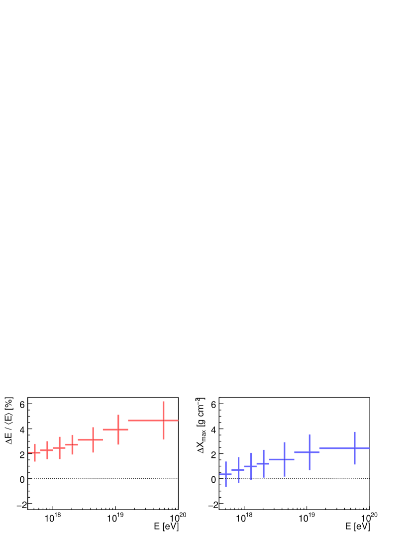
Figure 21: Overestimates of shower energy (left) and $X_{\text{max}}$ (right) due to lack of multiple scattering corrections in the hybrid reconstruction. The dotted lines correspond to a reconstruction with multiple scattering enabled. The uncertainties correspond to the sample RMS in each energy bin.

Figure 22: Systematic differences in shower energy (left) and $X_{\text{max}}$ (right) for events reconstructed using the multiple scattering corrections of Roberts [47] (dotted lines) and Pekala et al. [50].

6.4 Summary

Systematic Uncertainties
Source	$\log{(E/\text{eV})}$	$\Delta E/E$	RMS$(\Delta E/E)$	$\Delta X_{\text{max}}$	RMS$(X_{\text{max}})$
		(%)	(%)	($\text{g~{}cm}^{-2}$)	($\text{g~{}cm}^{-2}$)
Molecular Light Transmission and Production
Horiz. Uniformity	$17.7-20.0$	1	1	1	2
Quenching Effects	$17.7-20.0$	$+5.5$	$1.5-3.0$	$-2.0$	$7.2-8.4$
$p$, $T$, $u$ Variability	$17.7-20.0$	$-0.5$		$+2.0$
Aerosol Light Transmission
Optical Depth	$<18.0$	$+3.6$, $-3.0$	$1.6\pm 1.6$	$+3.3$, $-1.3$	$3.0\pm 3.0$
	$18.0-19.0$	$+5.1$, $-4.4$	$1.8\pm 1.8$	$+4.9$, $-2.8$	$3.7\pm 3.7$
	$19.0-20.0$	$+7.9$, $-7.0$	$2.5\pm 2.5$	$+7.3$, $-4.8$	$4.7\pm 4.7$
$\lambda$-Dependence	$17.7-20.0$	0.5	2.0	0.5	2.0
Phase Function	$17.7-20.0$	1.0	2.0	2.0	2.5
Horiz. Uniformity	$<18.0$	0.3	3.6	0.1	5.7
	$18.0-19.0$	0.4	5.4	0.1	7.0
	$19.0-20.0$	0.2	7.4	0.4	7.6
Scattering Corrections
Mult. Scattering	$<18.0$	0.4	0.6	1.0	0.8
	$18.0-19.0$	0.5	0.7	1.0	0.9
	$19.0-20.0$	1.0	0.8	1.2	1.1

Table 1: Systematic uncertainties in the hybrid reconstruction due to atmospheric influences on light transmission or production.

Table 1 summarizes our estimate of the impact of the atmosphere on the energy and $X_{\text{max}}$ measurements of the hybrid detector of the Pierre Auger Observatory. Aside from large quenching effects due to missing quenching corrections in the reconstruction, the systematic uncertainties are currently dominated by the aerosol optical depth: $4-8\%$ for shower energy, and about $4-8$ $\text{g~{}cm}^{-2}$ for $X_{\text{max}}$. This list of uncertainties is similar to that reported in [67], but now includes an explicit statement of the multiple scattering correction.

The RMS values in the table can be interpreted as the spread in measurements of energy and $X_{\text{max}}$ due to current limitations in the atmospheric monitoring program. For example, the uncertainties due to the variability of $p$, $T$, and $u$ are caused by the use of monthly molecular models in the reconstruction rather than daily measurements, while uncertainties due to the horizontal non-uniformity of aerosols are due to limited spatial sampling of the full atmosphere. Note that the RMS values listed for the aerosol optical depth are due to a mixture of systematic and statistical uncertainties; we have estimated these contributions conservatively by expressing the RMS as a central value with large systematic uncertainties. The combined values from all atmospheric measurements are, approximately, RMS($\Delta E/E$)$\approx 5\pm 1\%$ to $9\pm 1\%$ as a function of energy, and RMS($X_{\text{max}}$)$\approx 11\pm 1$ $\text{g~{}cm}^{-2}$ to $13\pm 1$ $\text{g~{}cm}^{-2}$. In principle, the RMS can be reduced by improving the spatial resolution and timing of the atmospheric monitoring data. Such efforts are underway, and are described in Section 7.

7 Additional Developments

We have estimated the uncertainties in shower energy and $X_{\text{max}}$ due to atmospheric transmission, but we have not discussed the impact of clouds on the hybrid reconstruction, which violate the horizontal uniformity assumption described in section 3.2. A full treatment of this issue will be the subject of future technical publications, but here we summarize current efforts to understand their effect on the hybrid data.

7.1 Cloud Measurements

Cloud coverage has a major influence on the reconstruction of air showers, but this influence can be difficult to quantify. Clouds can block the transmission of light from air showers, as shown in Figure 23, or enhance the observed light flux due to multiple scattering of the intense Cherenkov light beam. They may occur in optically thin layers near the top of the troposphere, or in thick banks which block light from large parts of the FD fiducial volume. The determination of the composition of clouds is nontrivial, making a priori estimates of their scattering properties unreliable.

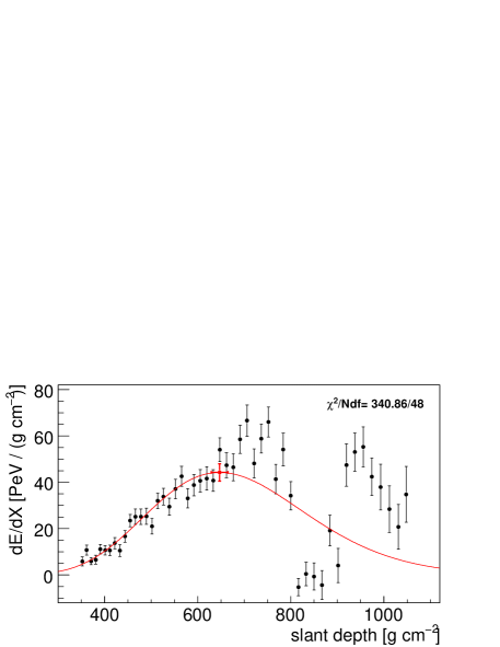
Figure 23: Shower light profile with a large gap due to the presence of an intervening cloud.

Due to the difficulty of correcting for the transmission of light through clouds, it is prudent to remove cloudy data using hard cuts on the shower profiles. But because clouds can reduce the event rate from different parts of a fluorescence detector, they also have an important effect on the aperture of the detector as used in the determination of the spectrum from hybrid data [61]. Therefore, it is necessary to estimate the cloud coverage at each FD site as accurately as possible.

Cloud coverage at the Pierre Auger Observatory is recorded by Raytheon 2000B infrared cloud cameras located on the roof of each FD building. The cameras have a spectral range of $7$ $\mu\text{m}$ to $14$ $\mu\text{m}$, and photograph the field of view of the six FD telescopes every 5 minutes during normal data acquisition. After the image data are processed, a coverage “mask” is created for each FD pixel, which can be used to remove covered pixels from the reconstruction. Such a mask is shown in fig. 24.

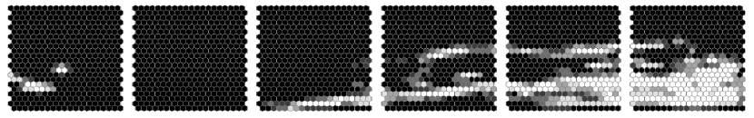
Figure 24: A mask of grayscale values used in the cloud database to indicate the cloud coverage of each pixel in an FD building. Lighter values indicate greater cloud coverage.

While the IR cloud cameras record the coverage in the FD field of view, they cannot determine cloud heights. The heights must be measured using the lidar stations, which observe clouds over each FD site during hourly two-dimensional scans of the atmosphere [21]. The Central Laser Facility can also observe laser echoes from clouds, though the measurements are more limited than the lidar observations. Cloud height data from the lidar stations are combined with pixel coverage measurements to improve the accuracy of cloud studies.

7.2 Shoot-the-Shower

When a distant, high-energy air shower is detected by an FD telescope, the lidars interrupt their hourly sweeps and scan the plane formed by the image of the shower on the FD camera. This is known as the “shoot-the-shower” mode. The shoot-the-shower mode allows the lidar station to probe for local atmospheric non-uniformities, such as clouds, which may affect light transmission between the shower and detector. Figure 25 depicts one of the four shoot-the-shower scans for the cloud-obscured event shown in fig. 23.

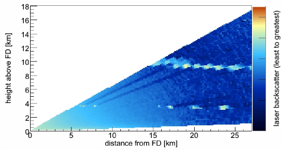
Figure 25: Lidar sweep of the shower-detector plane for the cloud-obscured event shown in fig. 23. The regions of high backscatter are laser echoes due to optically thick clouds.

A preliminary implementation of shoot-the-shower was described in [21]. This scheme has been altered recently to use a fast on-line hybrid reconstruction now operating at the Observatory. The new scheme allows for more accurate selection of showers of interest. In addition, the reconstruction output can be used to trigger other atmospheric monitors and services, such as radiosonde balloon launches, to provide measurements of molecular conditions shortly after very high energy air showers are recorded. “Balloon-the-shower” radiosonde measurements began at the Observatory in early 2009 [69].

8 Conclusions

A large collection of atmospheric monitors is operated at the Pierre Auger Observatory to provide frequent observations of molecular and aerosol conditions across the detector. These data are used to estimate light scattering losses between air showers and the FD telescopes, to correct air shower light production for various weather effects, and to prevent cloud-obscured data from distorting estimates of the shower energies, shower maxima, and the detector aperture.

In this paper, we have described the various light production and transmission effects due to molecules and aerosols. These effects have been converted into uncertainties in the hybrid reconstruction. Most of the reported uncertainties are systematic, not only due to the use of local empirical models to describe the atmosphere — such as the monthly molecular profiles — but also because of the nature of the atmospheric uncertainties — such as the systematics-dominated and highly correlated aerosol optical depth profiles.

Molecular measurements are vital for the proper determination of light production in air showers, and molecular scattering is the dominant term in the description of atmospheric light propagation. However, the time variations in molecular scattering conditions are small relative to variations in the aerosol component. The inherent variability in aerosol conditions can have a significant impact on the data if aerosol measurements are not incorporated into the reconstruction. Because the highest energy air showers are viewed at low elevation angles and through long distances in the aerosol boundary layer, aerosol effects become increasingly important at high energies.

Efforts are currently underway to reduce the systematic uncertainties due to the atmosphere, with particularly close attention paid to the uncertainties in energy and $X_{\text{max}}$. The shoot-the-shower program will improve the time resolution of atmospheric measurements, and increase the identification of atmospheric inhomogeneities that can affect observations of showers with the FD telescopes.

9 Acknowledgments

The successful installation and commissioning of the Pierre Auger Observatory would not have been possible without the strong commitment and effort from the technical and administrative staff in Malargüe.

We are very grateful to the following agencies and organizations for financial support: Comisión Nacional de Energía Atómica, Fundación Antorchas, Gobierno De La Provincia de Mendoza, Municipalidad de Malargüe, NDM Holdings and Valle Las Leñas, in gratitude for their continuing cooperation over land access, Argentina; the Australian Research Council; Conselho Nacional de Desenvolvimento Científico e Tecnológico (CNPq), Financiadora de Estudos e Projetos (FINEP), Fundação de Amparo à Pesquisa do Estado de Rio de Janeiro (FAPERJ), Fundação de Amparo à Pesquisa do Estado de São Paulo (FAPESP), Ministério de Ciência e Tecnologia (MCT), Brazil; AVCR AV0Z10100502 and AV0Z10100522, GAAV KJB300100801 and KJB100100904, MSMT-CR LA08016, LC527, 1M06002, and MSM0021620859, Czech Republic; Centre de Calcul IN2P3/CNRS, Centre National de la Recherche Scientifique (CNRS), Conseil Régional Ile-de-France, Département Physique Nucléaire et Corpusculaire (PNC-IN2P3/CNRS), Département Sciences de l’Univers (SDU-INSU/CNRS), France; Bundesministerium für Bildung und Forschung (BMBF), Deutsche Forschungsgemeinschaft (DFG), Finanzministerium Baden-Württemberg, Helmholtz-Gemeinschaft Deutscher Forschungszentren (HGF), Ministerium für Wissenschaft und Forschung, Nordrhein-Westfalen, Ministerium für Wissenschaft, Forschung und Kunst, Baden-Württemberg, Germany; Istituto Nazionale di Fisica Nucleare (INFN), Ministero dell’Istruzione, dell’Università e della Ricerca (MIUR), Italy; Consejo Nacional de Ciencia y Tecnología (CONACYT), Mexico; Ministerie van Onderwijs, Cultuur en Wetenschap, Nederlandse Organisatie voor Wetenschappelijk Onderzoek (NWO), Stichting voor Fundamenteel Onderzoek der Materie (FOM), Netherlands; Ministry of Science and Higher Education, Grant Nos. 1 P03 D 014 30, N202 090 31/0623, and PAP/218/2006, Poland; Fundação para a Ciência e a Tecnologia, Portugal; Ministry for Higher Education, Science, and Technology, Slovenian Research Agency, Slovenia; Comunidad de Madrid, Consejería de Educación de la Comunidad de Castilla La Mancha, FEDER funds, Ministerio de Ciencia e Innovación, Xunta de Galicia, Spain; Science and Technology Facilities Council, United Kingdom; Department of Energy, Contract No. DE-AC02-07CH11359, National Science Foundation, Grant No. 0450696, The Grainger Foundation USA; ALFA-EC / HELEN, European Union 6th Framework Program, Grant No. MEIF-CT-2005-025057, European Union 7th Framework Program, Grant No. PIEF-GA-2008-220240, and UNESCO.

References

- [1] A. Bunner, Cosmic Ray Detection by Atmospheric Fluorescence, Ph.D. thesis, Cornell University, Ithaca, New York (1967).
- [2] F. Arqueros, J. R. Hörandel, B. Keilhauer, Air Fluorescence Relevant for Cosmic-Ray Detection - Summary of the 5th Fluorescence Workshop, El Escorial 2007, Nucl. Instrum. Meth. A597 (2008) 1–22. arXiv:0807.3760[astro-ph].
- [3] R. M. Baltrusaitis, et al., The Utah Fly’s Eye Detector, Nucl. Instrum. Meth. A240 (1985) 410–428.
- [4] M. Unger, B. R. Dawson, R. Engel, F. Schussler, R. Ulrich, Reconstruction of Longitudinal Profiles of Ultra-High Energy Cosmic Ray Showers from Fluorescence and Cherenkov Light Measurements, Nucl. Instrum. Meth A588 (2008) 433–441. arXiv:0801.4309[astro-ph].
- [5] J. Linsley, in: Proc. 15th ICRC, Vol. 12, Plovdiv, Bulgaria, 1977, p. 89.
- [6] T. J. L. McComb, K. E. Turver, The Average Depth of Cascade Maximum in Large Cosmic Ray Showers from Particle Measurements, J. Phys. G8 (1982) 871–877.
- [7] B. Keilhauer, et al., Atmospheric Profiles at the Southern Pierre Auger Observatory and their Relevance to Air Shower Measurement, in: Proc. 29th ICRC, Vol. 7, Pune, India, 2005, pp. 123–127. arXiv:astro-ph/0507275.
-
[8]
The British Atmospheric Data Centre,
UK Met Office
Radiosonde Data.
URL {http://badc.nerc.ac.uk/data/radiosglobe/radhelp.html} - [9] B. Wilczyńska, et al., Variation of Atmospheric Depth Profile on Different Time Scales, Astropart. Phys. 25 (2006) 106–117. arXiv:astro-ph/0603088.
- [10] B. Keilhauer, et al., Impact of Varying Atmospheric Profiles on Extensive Air Shower Observation: Fluorescence Light Emission and Energy Reconstruction, Astropart. Phys. 25 (2006) 259–268. arXiv:astro-ph/0511153.
- [11] I. Tegen, A. A. Lacis, Modeling of Particle Size Distribution and its Influence on the Radiative Properties of Mineral Dust Aerosol, J. Geophys. Res. 101 (D14) (1996) 19,237–19,244.
- [12] U. Baltensperger, S. Nyeki, M. Kalberer, Atmospheric Particulate Matter, in: C. N. Hewitt, A. V. Jackson (Eds.), Handbook of Atmospheric Science, Blackwell, 2003, pp. 228–254.
- [13] S. Kinne, et al., An AeroCom Initial Assessment – Optical Properties in Aerosol Component Modules of Global Models, Atmos. Chem. Phys. 6 (2006) 1815–1834.
- [14] I. Allekotte, et al., The Surface Detector System of the Pierre Auger Observatory, Nucl. Instrum. Meth. A586 (2008) 409–420. arXiv:0712.2832[astro-ph].
- [15] J. Abraham, et al., The Fluorescence Detector of the Pierre Auger Observatory, submitted to NIM A (2009).
- [16] P. Sommers, Capabilities of a Giant Hybrid Air Shower Detector, Astropart. Phys. 3 (1995) 349–360.
- [17] T. Abu-Zayyad, et al., Measurement of the Cosmic Ray Energy Spectrum and Composition from eV to eV using a Hybrid Fluorescence Technique, Ap. J. 557 (2001) 686–699. arXiv:astro-ph/0010652.
- [18] M. Mostafá, Hybrid Activities of the Pierre Auger Observatory, Nucl. Phys. Proc. Suppl. 165 (2007) 50–58. arXiv:astro-ph/0608670.
- [19] B. R. Dawson, Hybrid Performance of the Pierre Auger Observatory, in: Proc. 30th ICRC, Vol. 4, Mérida, México, 2007, pp. 425–428. arXiv:0706.1105[astro-ph].
- [20] B. Fick, et al., The Central Laser Facility at the Pierre Auger Observatory, JINST 1 (2006) P11003.
- [21] S. Y. BenZvi, et al., The Lidar System of the Pierre Auger Observatory, Nucl. Instrum. Meth. A574 (2007) 171–184.
- [22] S. Y. BenZvi, et al., Measurement of the Aerosol Phase Function at the Pierre Auger Observatory, Astropart. Phys. 28 (2007) 312–320. arXiv:0704.0303[astro-ph].
- [23] S. Y. BenZvi, et al., Measurement of Aerosols at the Pierre Auger Observatory, in: Proc. 30th ICRC, Vol. 4, Mérida, México, 2007, pp. 355–358. arXiv:0706.3236[astro-ph].
- [24] S. Y. BenZvi, et al., New Method for Atmospheric Calibration at the Pierre Auger Observatory using FRAM, a Robotic Astronomical Telescope, in: Proc. 30th ICRC, Vol. 4, Mérida, México, 2007, pp. 347–350. arXiv:0706.1710[astro-ph].
- [25] L. Valore, Atmospheric Aerosol Measurements at the Pierre Auger Observatory, in: Proc. 31st ICRC, Łódź, Poland, 2009. arXiv:0906.2358[astro-ph].
- [26] F. Kakimoto, et al., A Measurement of the Air Fluorescence Yield, Nucl. Instrum. Meth. A372 (1996) 527–533.
- [27] M. Nagano, K. Kobayakawa, N. Sakaki, K. Ando, New Measurement on Photon Yields from Air and the Application to the Energy Estimation of Primary Cosmic Rays, Astropart. Phys. 22 (2004) 235–248. arXiv:astro-ph/0406474.
- [28] R. Abbasi, et al., The FLASH Thick-Target Experiment, Nucl. Instrum. Meth. A597 (2008) 37–40.
- [29] M. Bohacova, et al., A Novel Method for the Absolute Fluorescence Yield Measurement by AIRFLY, Nucl. Instrum. Meth. A597 (2008) 55–60. arXiv:0812.3649.
- [30] F. Arqueros, J. R. Hoerandel, B. Keilhauer, Air Fluorescence Relevant for Cosmic-Ray Detection - Review of Pioneering Measurements, Nucl. Instrum. Meth. A597 (2008) 23–31. arXiv:0807.3844.
- [31] M. Ave, et al., Measurement of the Pressure Dependence of Air Fluorescence Emission Induced by Electrons, Astropart. Phys. 28 (2007) 41. arXiv:astro-ph/0703132.
- [32] B. Keilhauer, J. Bluemer, R. Engel, H. O. Klages, Altitude Dependence of Fluorescence Light Emission by Extensive Air Showers, Nucl. Instrum. Meth. A597 (2008) 99–104. arXiv:0801.4200[astro-ph].
- [33] J. H. Seinfeld, S. N. Pandis, Atmospheric Chemistry and Physics: From Air Pollution to Climate Change, Wiley, 2006.
- [34] D. K. Killinger, N. Menyuk, Laser Remote Sensing of the Atmosphere, Science 235 (1987) 37–45.
- [35] J. Burris, T. J. McGee, W. Heaps, UV Raman Cross Sections in Nitrogen, Appl. Spec. 46 (1992) 1076.
- [36] A. Bucholtz, Rayleigh-Scattering Calculations for the Terrestrial Atmosphere, Appl. Opt. 34 (1995) 2765–2773.
- [37] H. Naus, W. Ubachs, Experimental Verification of Rayleigh Scattering Cross Sections, Opt. Lett. 25 (2000) 347–349.
- [38] G. Mie, A Contribution to the Optics of Turbid Media, Especially Colloidal Metallic Suspensions, Ann. Phys. 25 (1908) 377–445.
- [39] A. Ångstrøm, On the Atmospheric Transmission of Sun Radiation and on Dust in the Air, Geographical Analysis 12 (1929) 130–159.
- [40] E. J. McCartney, Optics of the Atmosphere, Wiley, 1976.
- [41] G. L. Schuster, O. Dubovik, B. N. Holben, Angstrom Exponent and Bimodal Aerosol Size Distributions, J. Geophys. Res. 111 (D10) (2006) 7207.
- [42] T. F. Eck, et al., Wavelength Dependence of the Optical Depth of Biomass Burning, Urban, and Desert Dust Aerosols, J. Geophys. Res. 104 (D24) (1999) 31333–31350.
- [43] D. C. B. Whittet, M. F. Bode, P. Murdin, The extinction properties of Saharan dust over La Palma, Vistas Astron. 30 (1987) 135–144.
- [44] E. S. Fishburne, M. E. Neer, G. Sandri, Voice Communication Via Scattered Ultraviolet Radiation, ARAP 274, Aeronautical Research Associates, Princeton, New Jersey (1976).
- [45] F. Riewe, A. E. S. Green, Ultraviolet Aureole Around a Source at a Finite Distance, Appl. Opt. 17 (1978) 1923–1929.
- [46] L. G. Henyey, J. L. Greenstein, Diffuse radiation in the Galaxy, Astrophys. J. 93 (1941) 70–83.
- [47] M. D. Roberts, The Role of Atmospheric Multiple Scattering in the Transmission of Fluorescence Light from Extensive Air Showers, J. Phys. G31 (2005) 1291–1301.
- [48] J. Pȩkala, D. Góra, P. Homola, B. Wilczyńska, H. Wilczyński, Contribution of Multiple Scattering of Cherenkov Photons to Shower Optical Image, in: Proc. 28th ICRC, Tsukuba, Japan, 2003, pp. 551–554.
- [49] M. Giller, A. Smialkowski, Multiple Scattering of the Fluorescence Light from EAS, in: Proc. 29th ICRC, Vol. 7, Pune, India, 2005, pp. 195–198.
- [50] J. Pekala, P. Homola, B. Wilczynska, H. Wilczynski, Atmospheric Multiple Scattering of Fluorescence and Cherenkov Light Emitted by Extensive Air Showers, Nucl. Instrum. Meth. A605 (2009) 388–398. arXiv:0904.3230[astro-ph].
-
[51]
Campbell Scientific, Inc., Weather
Stations.
URL {http://www.campbellsci.com/} - [52] C. Bleve, Weather Induced Effects on Extensive Air Showers Observed with the Surface Detector of the Pierre Auger Observatory, in: Proc. 30th ICRC, Vol. 4, Mérida, México, 2007, pp. 319–322. arXiv:0706.1491[astro-ph].
- [53] J. Abraham, et al., Atmospheric Effects on Extensive Air Showers Observed with the Surface Detector of the Pierre Auger Observatory, accepted for publication in Astropart. Phys. (2009).
-
[54]
Graw Radiosondes GmbH, Radiosonde DFM-97.
URL {http://www.graw.de/} - [55] L. Wiencke, Extracting First Science Measurements from the Southern Detector of the Pierre Auger Observatory, Nucl. Instrum. Meth. A572 (2007) 508–510. arXiv:astro-ph/0607449.
- [56] R. Abbasi, et al., Techniques for Measuring Atmospheric Aerosols at the High Resolution Fly’s Eye Experiment, Astropart. Phys. 25 (2006) 74–83. arXiv:astro-ph/0512423.
- [57] A. Filipčič, et al., Scanning Lidar Based Atmospheric Monitoring for Fluorescent Detectors of Cosmic Showers, Astropart. Phys. 18 (2003) 501–512.
- [58] E. Andrews, et al., Comparison of Methods for Deriving the Aerosol Asymmetry Parameter, J. Geophys. Res. 111 (D10) (2006) D05S04.
- [59] D. G. Kaskaoutis, et al., On the characterization of Aerosols using the Angstrom exponent in the Athens Area, J. Atmos. Solar-Terr. Phys. 68 (2006) 2147.
- [60] J. Allen, et al., The Pierre Auger Observatory Offline Software, J. Phys. Conf. Ser. 119 (2008) 032002. doi:10.1088/1742-6596/119/3/032002.
- [61] F. Schüssler, Measurement of the Cosmic Ray Energy Spectrum Above eV with the Pierre Auger Observatory, in: Proc. 31st ICRC, Łódź, Poland, 2009. arXiv:0906.2189[astro-ph].
- [62] C. Di Giulio, Energy Calibration of Data Recorded with the Surface Detectors of the Pierre Auger Observatory, in: Proc. 31st ICRC, Łódź, Poland, 2009. arXiv:0906.2189[astro-ph].
- [63] J. Bellido, Measurement of the Average Depth of Shower Maximum and its Fluctuations with the Pierre Auger Observatory, in: Proc. 31st ICRC, Łódź, Poland, 2009. arXiv:0906.2319[astro-ph].
- [64] U.S. Standard Atmosphere, COESA Report, U.S. Government Printing Office, Washington, D.C. (1976).
- [65] A. Morozov, et al., Eur. Phys. J. D33 (2005) 207.
- [66] T. Waldenmaier, J. Bluemer, H. Klages, Spectral Resolved Measurement of the Nitrogen Fluorescence Emissions in Air Induced by Electrons, Astropart. Phys. 29 (2008) 205–222. arXiv:0709.1494[astro-ph].
- [67] M. Prouza, in: Proc. 30th ICRC, Vol. 4, Mérida, México, 2007, pp. 351–354. arXiv:0706.1719[astro-ph].
- [68] J. Abraham, et al., Observation of the Suppression of the Flux of Cosmic Rays above eV, Phys. Rev. Lett. 101 (2008) 061101. arXiv:0806.4302[astro-ph].
- [69] B. Keilhauer, Rapid Monitoring of the Atmosphere at the Pierre Auger Observatory, in: Proc. 31st ICRC, Łódź, Poland, 2009. arXiv:0906.2358[astro-ph].