Complex networks: new trends for the analysis of brain connectivity

Abstract

Today, the human brain can be studied as a whole. Electroencephalography, magnetoencephalography, or functional magnetic resonance imaging (fMRI) techniques provide functional connectivity patterns between different brain areas, and during different pathological and cognitive neuro-dynamical states. In this Tutorial we review novel complex networks approaches to unveil how brain networks can efficiently manage local processing and global integration for the transfer of information, while being at the same time capable of adapting to satisfy changing neural demands.

1 Introduction

In recent years, complex networks have provided an increasingly challenging framework for the study of collective behaviors in complex systems, based on the interplay between the wiring architecture and the dynamical properties of the coupled units [1, 2]. Many real networks were found to exhibit small-world features. Small-world (SW) networks are characterized by having a small average distance between any two nodes, as random graphs, and a high clustering coefficient, as regular lattices  [3, 4, 5, 6]. Thus, a SW architecture is an attractive model for brain connectivity because it leads distributed neural assemblies to be integrated into a coherent process with an optimized wiring cost [7, 8, 9].

Another property observed in many networks is the existence of a modular organization in the wiring structure. Examples range from RNA structures, to biological organisms and social groups. A module is currently defined as a subset of units within a network such that connections between them are denser than connections with the rest of the network. It is generally acknowledged that modularity increases robustness, flexibility and stability of biological systems [10, 11]. The widespread character of modular architecture in real-world networks suggests that a network’s function is strongly ruled by the organization of their structural subgroups.

Recent studies have attempted to characterize the functional connectivity (patterns of statistical dependencies) observed between brain activities recorded by electroencephalography (EEG), magnetoencephalography (MEG), or functional magnetic resonance imaging (fMRI) techniques [12, 13, 14, 15, 16]. Surprisingly, functional connectivity patterns obtained from MEG and EEG signals during different pathological and cognitive neuro-dynamical states, were found to display SW attributes [15, 16]; whereas functional patterns of fMRI often display a structure formed by highly connected hubs, yielding an exponentially truncated power law in the degree distribution [12, 13, 14]. For a complete review of these issues, reader can refer to the Refs. [17, 18].

In functional networks, two different nodes (representing two electrodes, voxels or source regions) are supposed to be linked if some defined statistical relation exceeds a threshold. Regardless of the modality of recording activity (EEG, MEG or fMRI), topological features of functional brain networks are currently defined over long periods of time, neglecting possible instantaneous time-varying properties of the topologies. Nevertheless, evidence suggests that the emergence of a unified neural process is mediated by the continuous formation and destruction of functional links over multiple time scales [20, 19, 21].

Empirical studies have lead to the hypothesis that transient synchronization between distant and specific neural populations underlies the integration of neural activities as unified and coherent brain functions [19]. Specialized brain regions would be largely distributed and linked to form a dynamical web-like structure of the brain [20]. Thus, brain regions would be partitioned into a collection of modules, representing functional units, separable from -but related to- other modules. Characterizing the dynamical modular structure of the brain may be crucial to understand its organization during different pathological or cognitive states. An important question is whether the modular structure has a functional role on brain processes such as the ongoing awareness of sensory stimuli or perception.

To find the brain areas involved in a given cognitive task, clustering is a classical approach that takes into account the properties of the neurophysiological time series. Previous studies over the mammalian and human brain networks have successfully used different methods to identify clusters of brain activities. Some classical approaches, such as those based on principal components analysis (PCA) and independent components analysis (ICA), make very strong statistical assumptions (orthogonality and statistical independence of the retrieved components, respectively) with no physiological justification [22, 23].

In this Tutorial, we review an approach that allows to characterize the dynamic evolution of functional brain networks [24, 25]. We illustrate this approach on connectivity patterns extracted from MEG data recorded during a visual stimulus paradigm. Results reveal that the brain connectivity patterns vary with time and frequency, while maintaining a small-world structure. Further, we are able to reveal a non-random modular organization of brain networks with a functional significance of the retrieved modules. This modular configuration might play a key role in the integration of large scale brain activity, facilitating the coordination of specialized brain systems during a cognitive brain process.

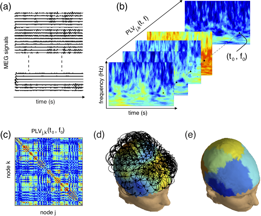
Figure 1: General scheme for the extraction of the time-varying brain networks: (a) signals are decomposed into time-frequency components to compute (b) pair-wise relations; (c) functional connectivity matrices are extracted at each point of the time-frequency space, defining (d) the functional brain networks used to extract the topological attributes (color codes the nodes degree) and the (e) modular structure (brain sites belonging to each module are arbitrarily colored). See details in the text.

2 Materials and methods

To illustrate our approach, we consider the brain responses recorded during the visual presentation of non-familiar pictures. Although our approach is applicable to any of the functional methods available (EEG, fMRI, MEG), here we use the magnetoencephalography. This modality of acquisition has the major feature that collective neural behaviors, as synchronization of large and sparsely distributed cortical assemblies, are reflected as interactions between MEG signals [26]. We study the functional connectivity patterns associated with dynamic brain processes elicited by the repetitive application (trials) of a external visual stimulus [27]. For this experiment, a collection of $48$ simple structural images and scrambled images were randomly shown to epileptic patients for a periode of $150$ ms with an inter-stimulus interval of $2$ s. Patients were required to respond by pressing a button each time an image was perceived. The event-related brain responses were recorded (from two patients) with a whole-head MEG system (151 sensors; VSM MedTech, Coquitlam, BC, Canada) digitized at $1.25$ kHz with a bandpass of $0-200$ Hz.

The basic steps of our approach are schematically illustrated in Fig. 1. Each of the signals is decomposed into time-frequency components, as shown in panel a). The relations between two signals $j$ and $k$ are firstly defined in time-frequency space, as shown in panel b). A statistical criterion is then used to define a functional connectivity matrix for each time-frequency point, panel c). The details of the statistical criterion we adopted are reported in Section 2.1. In panel d), topological metrics are extracted from the connectivity patterns to obtain a time-frequency characterization of brain networks. The metrics investigated are analyzed in Section 2.2. Finally, in panel e), at a given frequency, or time instant of interest, the modular structure is characterized as discussed in Sections 2.3 and 2.4. To evaluate the features of brain connectivity, the obtained functional networks are compared with equivalent regular and random networks.

2.1 Estimation of functional connectivity

A unified definition of brain connectivity is difficult from the fact that the recorded dynamics reflect the activities of neural networks at different spatial and temporal resolutions. Three types of connectivity are currently considered: anatomical (description of the physical connections between two brain sites), functional (defined by a temporal correlation between distant neurophysiological events) and effective (causal influence that a neural system may exert over another). Here, we consider the functional links in brain signals defined by means of the phase-locking value (PLV) computed between all pairs of sensors [28]. To compute the PLV values, we used a complex Morlet’s wavelet function defined as $w(t,f_{0})=A\exp(-t^{2}/2\sigma_{t}^{2})\times\exp(i2\pi f_{0}t)$. Normalization factor $A$ was set to $A=(\sigma_{t}\sqrt{\pi})^{-1/2}$. $\sigma_{t}=m/2\pi f_{0}$, $m$ is a constant that defines the compromise between time and frequency resolution, and $f_{0}$ is the center frequency of the wavelet. Hence, in time domain, its real and imaginary parts are a cosine and a sine, respectively, of which the amplitude envelope is a Gaussian with a standard deviation of $\sigma_{t}$. In frequency domain, the Morlet wavelet is also a Gaussian with a standard deviation $\sigma_{f}$ given $m=f_{0}/\sigma_{f}$. Here, $m$ was chosen to be 7. By means of this complex wavelet transform an instantaneous phase $\phi_{i}^{trial}(t,f)$ is obtained for each frequency component of signals $i=1,\ldots,M$ at each repetition of the stimulus (trial). The PLV between any pair of signals $(i,k)$ is inversely related to the variability of phase differences across trials:

$$\text{PLV}_{i,k}(t,f)=\\ \phantom{=}\frac{1}{N_{trials}}\left|\sum_{trial=1}^{N_{trials}}\exp^{j(\phi_{i}^{trial}(t,f)-\phi_{k}^{trial}(t,f))}\right|,$$

where $N_{trials}$ is the total number of trials. If the phase difference varies little across trials, its distribution is concentrated around a preferred value and $\text{PLV}\sim 1$. In contrast, under the null hypothesis of a uniformity of phase distribution, PLV values are close to zero.

Finally, to assess whether two different sensors are functionally connected, we calculated the significance probability of the PLV values by a Rayleigh test of uniformity of phase. According to this test, the significance of a PLV value determined from $N_{trials}$ can be calculated as $p=\exp(-N_{trials}\text{PLV}^{2})$ [29]. To correct for multiple testing, the False Discovery Rate (FDR) method was applied to each matrix of PLV values [30]. With this approach, the threshold of significance $PLV_{th}$ was set such that the expected fraction of false positives is restricted to $q\leq 0.05$.

In the construction of the networks, a functional connection between two brain sites was assumed as an undirected and unweighted edge ($A_{ij}=1$ if $PLV_{ij}>PLV_{th}$; and zero otherwise). Although topological features can also be straightforwardly generalized to weighted networks  [32], we obtained qualitative similar results (not reported here) for weighted networks with a functional connectivity strength between nodes given by $w_{ij}=PLV_{ij}$. More refined statistical tools can also be used to estimate time-varying and directed brain networks [31].

2.2 Time-varying structure of brain networks

A set of metrics can be used to characterize the topological properties of the functional networks we have constructed [1, 2]. Here, we use three key parameters: mean degree $\langle K\rangle$, clustering index $C$ and global efficiency $E$. Briefly, the degree $k_{i}$ of node $i$ denotes the number of functional links incident with the node and the mean degree is obtained by averaging $k_{i}$ across all nodes of the network. The clustering index quantifies the local density of connections in a node’s neighborhood. The clustering coefficient $c_{i}$ of a node $i$ is calculated as the number of links between the node’s neighbors divided by all their possible connections and $C$ is defined as the average of $c_{i}$ taken over all nodes of the network [3]. The global efficiency $E$ provides a measure of the network’s capability for information transfer between nodes and is defined as the inverse of the harmonic mean of the shortest path length $L_{ij}$ between each pair of nodes [6]. The node-efficiency $E_{i}$ of the $i^{\text{th}}$ node is likewise defined as the inverse of the harmonic mean of the minimum path length between node $i$ and all other nodes in the network.

To asses the small-world behavior of functional networks, we perform a benchmark comparison of the functional connectivity patterns [3]. For this, the clustering and efficiency coefficients of functional networks are compared with those obtained from equivalent random and regular configurations. Regular networks were obtained by rewiring the links of each node to its nearest (in the sensors space) neighbors, yielding a nearest-neighbor connectivity with the same degree distribution as the original network. To create an ensemble of equivalent random networks we use the algorithm described in Ref. [3]. According to this procedure, each edge of the original network is randomly rewired avoiding self and duplicate connections. The obtained randomized networks preserve thus the same mean degree as the original network whereas the rest of the wiring structure is random.

2.3 Network modularity

Many real networks have a modular structure, i.e. their associated graphs are in general globally sparse but locally dense. In these networks, modules are defined as groups of vertices linked such that connections between them are denser than connections with the rest of the network. It is currently accepted that a partition $\mathcal{P}=\{\mathcal{C}_{1},\ldots,\mathcal{C}_{M}\}$ represents a good division in modules if the portion of edges inside each module $\mathcal{C}_{i}$ (intra–modular edges) is high compared to the portion of edges between them (inter–modular edges). The modularity $Q(\mathcal{P})$, for a given partition $\mathcal{P}$ of a network is formally defined as [33]:

$$Q(\mathcal{P})=\sum_{s=1}^{M}{\left[{\frac{l_{s}}{L}-\left(\frac{k_{s}}{2L}\right)}^{2}\right]},$$ (1)

where $M$ is the number of modules, $L$ is the total number of connections in the network, $l_{s}$ is the number of connections between vertices in module $s$, and $k_{s}$ is the sum of the degrees of the vertices in module $s$.

To partition the functional networks in modules, we used a random walk-based algorithm [34], because of its ability to manage very large networks, and its good performances in benchmark tests [34, 37]. Similar theoretical frameworks have been recently proposed for spectral coarse-graining [35, 36]. The algorithm is based on the intuition that a random walker on a graph tends to remain into densely connected subsets corresponding to modules. Let $P_{ij}=\frac{A_{ij}}{k_{i}}$ to be the transition probability from node $i$ to node $j$, where $A_{ij}$ denotes the adjacency matrix and $k_{i}$ is the degree of the i^th node. This defines the transition matrix $(P^{t})_{ij}$ for a random walk process of length $t$ (denoted here $P^{t}_{ij}$ for simplicity). One can notice that, if two vertices $i$ and $j$ are in the same community, the probability $P^{t}_{ij}$ is high, and $P^{t}_{ik}\simeq P^{t}_{jk}\forall k$.

The metric used to quantify the structural similarity between vertices is given by

$$\rho_{ij}=\sqrt{\sum_{l=1}^{N}\frac{(P^{t}_{il}-P^{t}_{jl})^{2}}{k_{l}}}$$ (2)

This distance has several advantages: it quantifies the structural similarity between vertices and it can be used in an efficient clustering algorithm to maximize the network modularity $Q$. Further, using matrix identities, the distance $\rho$ can be written as $\rho^{2}_{ij}=\sum^{n}_{\alpha=2}{\lambda^{2t}_{\alpha}{(v_{\alpha}(i)-v_{\alpha}(j))}^{2}}$; where $(\lambda_{\alpha})_{1\leqslant\alpha\leqslant n}$ and $(v_{\alpha})_{1\leqslant\alpha\leqslant n}$ are the $n$ eigenvalues and right eigenvectors of the matrix $P$, respectively [34]. This relates the random walk algorithm to current methods using spectral properties of the graphs [38, 36]. The random-walk based approach, however, needs not to explicitly compute the eigenvectors of the matrix; a computation that rapidly becomes intractable when the size of the graphs exceeds some thousands of vertices.

To find the modular structure, the algorithm starts with a partition in which each node in the network is the sole member of a module. Modules are then merged by an agglomerative approach based on a hierarchical clustering method [39]. The algorithm stops when all the nodes are grouped into a single component. At each step the algorithm evaluates the quality of partition $Q$. The partition that maximizes $Q$ is considered as the partition that better captures the modular structure of the network. In the calculation of $Q$, the algorithm excludes small isolated groups of connected vertices without any links to the main network. However, these isolated modules are considered here as part of the network for the calculation of the topological parameters.

2.4 Comparison of network partitions

To evaluate the agreement between modules assignments at a given time instant or frequency one can used the adjusted Rand index $Ra$ [41], which is a traditional criterion for comparison of different results provided by classifiers and clustering algorithms, including partitions with different numbers of classes or clusters. For two partitions $P$ and $P^{\prime}$, the original Rand index is defined as [40] $R=\frac{a+d}{a+b+c+d}$; where $a$ is number of pairs of data objects belonging to the same class in $P$ and to the same class in $P^{\prime}$, $b$ is number of pairs of data objects belonging to the same class in $P$ and to different classes in $P^{\prime}$, $c$ is the number of pairs of data objects belonging to different classes in $P$ and to the same class in $P^{\prime}$, and $d$ is number of pairs of data objects belonging to different classes in $P$ and to different classes in $P^{\prime}$. Thus the index $R$ has a straightforward interpretation as a percentage of agreement between the two partitions and it yields values between $0$ (if the two partitions are randomly drawn) and $1$ (for identical partition structures).

The Rand index, however, has a bias if a partition is composed by many clusters, and it can take a non-null value for two completely random partitions. The index $R$ can be straightforwardly corrected for the expected value under the null hypothesis according to the following general scheme: $Ra=\frac{R-E\{R\}}{\max\{R\}-E\{R\}}$. Using the generalized hypergeometric distribution as the null hypothesis, the adjusted Rand index that corrects for the expected number of nodes pairs placed in the same module under two random partitions is given by [41]

$$Ra=\frac{a-\frac{(a+c)(a+b)}{a+b+c+d}}{\frac{2a+b+c}{a+b+c+d}-\frac{(a+c)(a+b)}{a+b+c+d}}$$ (3)

which has an expected value of zero under the null hypothesis, and it takes a maximum value of one for a perfect agreement of the two partitions. Thus, the adjusted Rand index is a statistics on the level of agreement or correlation between two partitions.

3 Results

3.1 Time-frequency dependence of brain networks

Fig. 2 shows the topological attributes of functional networks elicited by the -unexpected- images. Pictures show the values of the mean degree, clustering index and efficiency of networks between, calculated at each point of the time-frequency space, $600$ ms before and $1$ s after the onset of the stimulus.

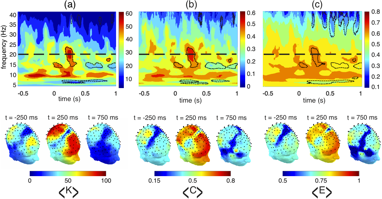
Figure 2: Time-frequency maps of topological features extracted from brain networks associated to a visual stimulus presentation (arriving at $t=0$). (a) mean degree $\langle K\rangle$, (b) clustering index $C$ and (c) efficiency $E$. The reported values refer to the average over subjects. Dotted lines outline the regions revealing a significant change from the pre-stimulus region. Lower row: topographic distribution of the local parameters for the 20 Hz activities (indicated by the thick dashed line) at three different time instants.

The first crucial observation is that functional connectivity patterns are not time-invariant, but instead they exhibit a rich time-frequency structure during the neural processing. All the topological features (specially $\langle K\rangle$ and $C$) exhibit high values in a frequency band close to $10$ Hz, which is a spectral component mostly involved in the processing of visual information [27]. Whereas the functional networks in the frequency range of $10-30$ Hz display large patterns of synchronization/desynchronization before the stimuli, a highly connected pattern is induced by the stimulus at about $250$ ms and between $15$ and $25$ Hz, suggesting a connectivity induced by the unexpected sensory stimuli. This is followed by weak connected structures at frequency bands close to $7$ and $15$ Hz arising during the post-stimulus activities and marking the transition between the moment of perception and the motor response of the subject. The topological features of these connectivity patterns were detected as statistically different from the pre-stimulus epoch by a $Z$-test corrected by a FDR at $q\leq 0.05$. Brain activities above $30$ Hz are characterized by a poor global connectivity. Local parameters, $k_{i}$, $c_{i}$ and $E_{i}$, for each sensor of the network are shown at three different time instants for a frequency of $20\ Hz$. During the processing of the stimulus, a time-space variability of connectivity is observed. Before the onset of the stimulus, the networks are characterized by a very sparse connectivity. Then, a clear clustered structure triggered by the stimulus appears at $t=250$ ms, defining two main regions (frontal and occipital) with a high density of connections. After the stimulus, the functional wiring displays again a sparse structure.

3.2 Small-world behavior of brain networks

The comparison of the brain networks against random and regular configurations is shown Fig. 3. Typically, small-world networks exhibit a $E_{sw}$ greater than regular lattices, but less than random wirings $E_{lat}<E_{sw}<E_{rnd}$; while for the mean cluster index, $C_{rnd}<C_{sw}<C_{lat}$ is expected [3]. Results reveal that, despite the variability observed, functional networks display a topology different from regular and random networks. Namely, $\frac{C}{\langle C_{rnd}\rangle}>1$ and $\frac{C}{\langle C_{lat}\rangle}<1$, which indicates a SW structure ($\langle...\rangle$ stays for an average over the ensembles of equivalent networks). Further, $\frac{\langle E_{lat}\rangle}{E}<1$ and $\frac{\langle E_{rnd}\rangle}{E}>1$, supporting the hypothesis of a SW connectivity.

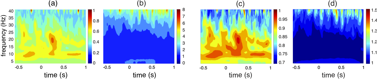
Figure 3: Comparison of functional networks with random and regular configurations: time-frequency maps of (a) $C/\langle C_{lat}\rangle$, (b) $C/\langle C_{rnd}\rangle$, (c) $\langle E_{lat}\rangle/E$ and (d) $\langle E_{rnd}\rangle/E$. Results of equivalent random and regular networks refer to the average of $20$ realizations.

It is important to emphasize that, in contrast with previous studies which have focused on time-invariant networks [12, 13, 14, 15, 16], our approach reveals a dynamical small-world connectivity at multiple time scales. This is a remarkable result, insofar as it suggests that the processing of a stimulus involves an optimized (in a SW sense) functional integration of distant brain regions by a dynamic reconfiguration of links.

3.3 Evolution of functional modules

A potential modularity of brain-webs is suggested by the fact that brain networks display a clustering index larger than that obtained from random configurations [42]. Indeed, the presence of modules is actually confirmed by the high values of $Q$ obtained for brain networks extracted from brain activities at different time instants and frequencies. Fig. 4 shows the spatial distribution of the modules for different networks with the following $Q$ values: (a) $Q=0.55$, (b) $Q=0.33$, (c) $Q=0.53$, (d) $Q=0.53$, (f) $Q=0.49$ and (g) $Q=0.53$.

Results show that brain networks have a time-varying structure with a number of modules that changes with time and frequency. From plots one can observe that, despite the spatial variability observed at different time instants and frequencies, functional modules fit well some known brain regions including visual, somatosensory and auditory processing areas. Before the onset of the stimulus, however, networks are characterized by modular structures that define four main regions (anterior and posterior for both left and right hemisphere). We notice that the partitions of both networks present a relatively low agreement yielding a $Ra=0.39$. Then, the large connectivity triggered by the stimulus is also accompanied by an increase in the number of modules, yielding a more complex modular structure. The observed changes are directly related with the specific nature of the task:the detection and low-level processing of the stimulus involves the visual system, but further processing as the identification and perception of the picture requires the mediation of regions as those located in frontal regions. Surprisingly antero-posterior relations elicit a large and unique module fitting fronto-occipital regions. Although a one-to-one assignment of anatomo-functional roles to each detected module is difficult to define, results reveal some other interesting modules, as the ones located over the motor cortex at $f=18.5$ Hz. Then the post-stimulus activities recovers again a simpler spatial organization of modules. It is worthy to notice that the pre- and post-stimulus networks have a very similar modular architecture only for the brain activities at the frequency band of $10$ Hz. This high agreement is confirmed by a high value of the adjusted Rand index ($Ra=0.626$), compared with the values less than $0.38$ obtained for other frequencies.

These are remarkable results as they support the hypothesis that brain dynamics relies on different modular organizations to integrate distant specialized, but functionally related, brain regions. Our findings suggest modularity as an organization basis leading distributed groups of specialized neural assemblies to be integrated into a coherent process during different cognitive or pathological states. A modular description of brain networks might provide, more in general, meaningful insights into the functional organization of brain activities during others neural functions, such as attention and consciousness.

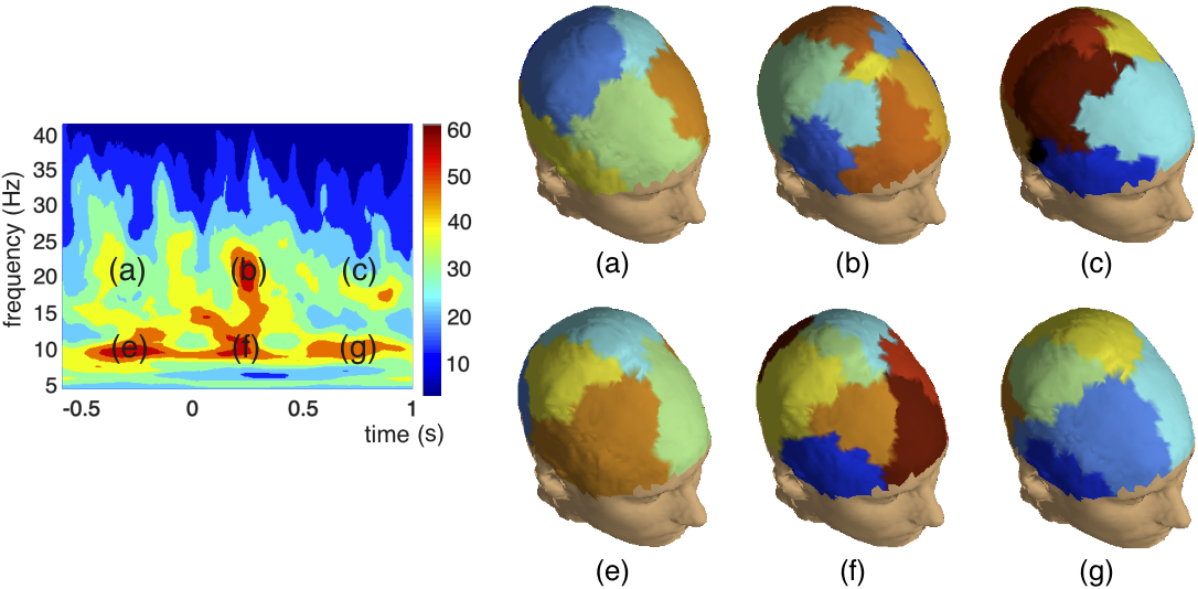
Figure 4: Topographical distribution of the modules extracted from brain networks at different time instants and frequencies: (a) time instant t = -0.25 s, frequency f =20 Hz; (b) t = 0.25 s after the presentation of the stimulus at f =20 Hz; (c) t =0.75 s, f =20 Hz; (e) t =-0.25 s, f =10 Hz; (f) t =0.25 s, f =10 Hz and (g) t =0.75 s, f =10 Hz. Brain sites belonging to each functional brain module were arbitrarily colored (there is no color correspondence between the modules of different networks). For the sake of clarity, isolated nodes were colored in black. (d) Time-frequency maps of mean degree is plotted to help network’s localization in the time frequency space

4 Conclusion

In this Tutorial we have addressed a fundamental problem in brain networks research: whether and how brain behavior relies on the coordination of a dynamic mosaic of functional brain modules during cognitive states. We have proposed a method to study the time-frequency dependencies of functional brain networks, thus offering an instantaneous description of the brain architecture. Applied to a visual stimulus paradigm, the method reveals that the functional brain connectivity evolves in a small-world structure during the different episodes of the neural processing. Furthermore, by using a random walk-based analysis, we have identified a non-random modular structure in the functional brain connectivity.

The present analysis was performed on MEG data in sensor space, which contains some inherent spurious correlation between magnetic fields on the surface of the brain. Although this caveat does not affect the characterization of the global network topology, accurate inferences about anatomical locations needs a source reconstruction of the activity in the cortex. In this study, we have reduced the influence of spurious correlations by simply excluding the nearest sensors from the computation of PLV values.

Our approach may provide meaningful insights into how brain networks can efficiently manage a local processing and a global integration for the transfer of information, while being at the same time capable of adapting to satisfy changing neural demands. Although the neurophysiological mechanisms involved in the functional integration of distant brain regions are still largely unknown, a dynamic SW organization is a plausible solution to the apparently opposing needs of local specificity of activity versus the constraints imposed by the coordination of distributed brain areas. The modular structure constitutes therefore an attractive model for the brain organization as it supports the coexistence of a functional segregation of distant specialized areas and their integration during brain states [4, 5]. We suggest that this network description might provide new insights into the understanding of human brain connectivity during pathological or cognitive states.

Applied to other multivariate data, our approach could provide new insights into the structure of the time-varying connectivity at a certain time [24]. A modular description of brain networks might provide, more in general, meaningful insights into the functional organization of brain activities recorded with others neuroimaging techniques (EEG, MEG or fMRI) during diverse cognitive or pathological states [25]. In this study, the functional links have been defined in MEG signals by means of the phase-locking value. We notice, however, that other time-frequency methods (e.g. wavelet cross-spectra) can also be used to detect and characterize a time-varying connectivity of spatially extended, nonstationary systems (e.g. financial or epidemiological networks).

5 Acknowledgments

The authors would like to thank S. Dupont, A. Ducorps and G. Yvert for clinical and technical support during data acquisition. This work was supported by the EU-GABA contract no. 043309 (NEST) and CIMA-UTE projects.

References

- [1] M. E. J. Newman [2003] “The structure and function of complex networks”, SIAM Rev. 45, 167-256.
- [2] S. Boccaletti, V. Latora, Y. Moreno, M. Chavez and D.-U. Hwang [2006] “Complex Networks : Structure and Dynamics”, Phys. Rep. 424, 175-308.
- [3] D. J. Watts and S. H. Strogatz [1998] “Collective dynamics of small-world’ networks”, Nature (London) 393, 440-442.
- [4] G. Tononi, G. M. Edelman and O. Sporns [1998] “Complexity and coherency: Integrating information in the brain”, Trends Cogn. Sci. 2, 474-484.
- [5] O. Sporns, G. Tononi and G. M. Edelman [2000] “Theoretical neuroanatomy: relating anatomical and functional connectivity in graphs and cortical connection matrices”, Cerebral Cortex 10, 127-141.
- [6] V. Latora and M. Marchiori [2001] “Efficient behavior of small-world networks”, Phys. Rev. Lett. 87, 198701.
- [7] V. Latora and M. Marchiori [2003] “Economic small-world behavior in weighted networks”, Eur. Phys. J. B 32, 249-263.
- [8] G. Buzsáki, C. Geisler, D. A. Henze, and X. J. Wang [2004] “Interneuron Diversity series: Circuit complexity and axon wiring economy of cortical interneurons”, Trends Neurosci. 27, 186-193.
- [9] O. Sporns, D. R. Chialvo, M. Kaiser, and C. C. Hilgetag [2004] “Organization, development and function of complex brain networks”, Trends Cogn. Sci. 8, 418-425.
- [10] A. L. Barabási and Z. N. Oltvai [2004] “Network biology: understanding the cell’s functional organization”, Nat. Rev. Genet. 5, 101-113.
- [11] R. V. Solé and S. Valverde [2008] “Spontaneous emergence of modularity in cellular networks.” J. R. Soc. Interface 5, 129-133.
- [12] V. M. Eguíluz, D. R. Chialvo, G. A. Cecchi, M. Baliki and A. V. Apkarian [2005] “Scale-free brain functional networks”, Phys. Rev. Lett. 94, 018102.
- [13] S. Achard, R. Salvador, B. Whitcher, J. Suckling and E. Bullmore [2006] “A resilient, low-frequency, small-world human brain functional network with highly connected association cortical hubs”, J. Neurosci. 26, 63-72.
- [14] S. Achard and E. Bullmore [2007] “Efficiency and cost of economical brain functional networks”, PLoS Comput. Biol. 3, e17.
- [15] D. S. Bassett, A. Meyer-Lindenberg, S. Achard, T. Duke and E. Bullmore [2006] “Adaptive reconfiguration of fractal small-world human brain functional networks”, Proc. Natl. Acad. Sci. USA, 103, 19518-19523.
- [16] C. J. Stam, B. F. Jones, G. Nolte, M. Breakspear and P. Scheltens [2007] “Small-world networks and functional connectivity in Alzheimer’s disease”, Cereb Cortex 17, 92-99.
- [17] J. C. Reijneveld, S. C. Ponten, H. W. Berendse, and C. J. Stam, [2007] “The application of graph theoretical analysis to complex networks in the brain”, Clin. Neurophysiol. 118, 2317 2331.
- [18] E. Bullmore and O. Sporns [2007] “Complex brain networks: graph theoretical analysis of structural and functional systems”, Nat. Rev. Neurosci. 10, 1-13.
- [19] A. K. Engel, P. Fries and W. Singer [2001] “Dynamic predictions: oscillations and synchrony in top-down processing”, Nat. Rev. Neurosci. 2, 704-716.
- [20] F. Varela, J.-P. Lachaux, E. Rodriguez and J. Martinerie [2001] “The brainweb: phase synchronization and large-scale integration”, Nat. Rev. Neurosci. 2, 229-239.
- [21] C. J. Honey, R. Kötter, M. Breakspear and O. Sporns [2007] “Network structure of cerebral cortex shapes functional connectivity on multiple time scales”, Proc. Natl. Acad. Sci. USA, 104, 10240-10245.
- [22] B. B. Biswal and J. Ulmer [1999] “Blind source separation of multiple signal sources of fMRI data sets using independent component analysis”, J. Comput. Assist. Tomo. 23, 265-271.
- [23] M. McKeown, L. Hansen, and T. Sejnowski [2003] “Independent Component Analysis of functional MRI: What Is Signal and What Is Noise? ”, Curr. Opin. Neurobiol. 13, 620-629.
- [24] M. Valencia, S. Dupont, J. Martinerie, and M. Chavez [2008] “Dynamic small-world behavior in functional brain networks unveiled by an event-related networks approach”, Phys Rev E 77, 050905-R
- [25] M. Valencia, M. A. Pastor, M. A. Fernández-Seara, J. Artieda, J. Martinerie, and M. Chavez [2009] “Complex modular structure of large-scale brain networks”, Chaos. 19, 02311.
- [26] M. Hämäläinen, R. Hari, R. Ilmoniemi, J. Knuutila and O. V. Lounasmaa [1993] “Magnetoencephalography- theory, instrumentation, and applications to noninvasive studies of the working human brain”, Rev. Mod. Phys. 65, 413-497.
- [27] D. Regan [1989]. Human brain electrophysiology: Evoked potentials and evoked magnetic fields in Science and medicine (Elsevier, New York).
- [28] J.-P. Lachaux, E. Rodriguez, J. Martinerie and F. J. Varela [1999] “Measuring phase synchrony in brain signals”, Human Brain Mapping 8 194-208.
- [29] N. I. Fisher [1989]. Statistical analysis of circular data (Cambridge University Press, UK).
- [30] Y. Benjamini, and Y. Hochberg [1995] “Controlling the False Discovery Rate: A Practical and Powerful Approach to Multiple Testing”, J. R. Statist. Soc. B 57, 289-300.
- [31] F. De Vico Fallani, V. Latora, L. Astolfi, F. Cincotti, D. Mattia, M. G. Marciani, S. Salinari, A. Colosimo and F. Babiloni [2008] “Persistent patterns of interconnection in time-varying cortical networks estimated from high-resolution EEG recordings in humans during a simple motor act”, J. Phys. A: Math. Theor. 41, 224014.
- [32] A. Barrat, M. Bartélemy, R. Pastor-Satorras, and A. Vespignani [2004] “The architecture of complex weighted networks”, Proc. Natl. Acad. Sci. USA 101, 3747-3752.
- [33] M. E. J. Newman and M. Girvan [2004] “Finding and evaluating community structure in networks”, Phys. Rev. E. 69, 026113.
- [34] M. Latapy and P. Pons [2006] “Computing Communities in Large Networks Using Random Walks”, Journal of Graph Algorithms and Applications 10, 191-218.
- [35] C. Allefeld and S. Bialonski [2006] “Detecting synchronization clusters in multivariate time series via coarse-graining of Markov chains”, Phys. Rev. E. 76, 066207.
- [36] D. Gfeller and P. De Los Rios [2007] “Spectral coarse graining of complex networks” Phys. Rev. Lett. 99, 038701.
- [37] L. Danon, A. Díaz-Guilera, J. Duch and A. Arenas [2005] “Comparing community structure identification”, J Stat. Mech. P09008.
- [38] M. E. J. Newman [2006] “Finding community structure in networks using the eigenvectors of matrices”, Phys. Rev. E. 74, 036104.
- [39] J. H. Ward [1963] “Hierarchical grouping to optimize an objective function”, J. Am. Statist. Assoc. 58, 236-244.
- [40] W. M. Rand [1971] “Objective criteria for the evaluation of clustering methods”, J. Am. Statist. Assoc. 66, 846-850.
- [41] L. Hubert and P. Arabie [1985] “Comparing partitions”, J. Classif. 2, 193-218.
- [42] E. Ravasz, A. L. Somera, D. A. Mongru, Z. N. Oltvai, and A.-L. Barabási [2002] “Hierarchical Organization of Modularity in Metabolic Networks”, Science 297, 1551-1555.