Reciprocity of mobile phone calls

Lauri Kovanen, Jari Saramäki, Kimmo Kaski
Department of Biomedical Engineering and Computational Science
Aalto University School of Science and Technology, Finland
lauri.kovanen@tkk.fi

Abstract

We present a study of the reciprocity of human behaviour based on mobile phone usage records. The underlying question is whether human relationships are mutual, in the sense that both are equally active in keeping up the relationship, or is it on the contrary typical that relationships are lopsided, with one party being significantly more active than the other. We study this question with the help of a mobile phone data set consisting of all mobile phone calls between 5.3 million customers of a single mobile phone operator. It turns out that lopsided relations are indeed quite common, to the extent that the variation cannot be explained by simple random deviations or by variations in personal activity. We also show that there is no non-trivial correlation between reciprocity and local network density.

1 Introduction

Representing collections of social relations as networks has become a standard practice not only in sociology but also in the study of complex systems. A social network $G=(V,E)$ is defined by the set of $N$ nodes, $V=\{v_{i}\}_{i=1}^{N}$ , which correspond to individuals, and by the set of edges (or links) $E=\{e_{ij}=(v_{i},v_{j}),\,v_{i},v_{j}\in V\}$ , which correspond to some associations between the individuals. Even though it is common to assume the associations to be symmetric (i.e. $e_{ij}=e_{ji}$ ) [1, 2, 3], for our purposes the edges are always directed, meaning that $e_{ij}$ is independent of $e_{ji}$ . In a weighted network each edge is also assigned a weight. We consider the edge weights as proxies for the strength of a relationship, and therefore the weights are strictly positive. In our notation $w_{ij}>0$ is the weight of a directed edge from node $v_{i}$ to $v_{j}$ , and $w_{ij}=0$ is equivalent to saying that there is no edge from $v_{i}$ to $v_{j}$ .

We use the term reciprocity to depict the degree of mutuality of a relationship. A relationship with a high reciprocity is one where both are equally interested in keeping up the relationship — a good example is the relationship of Romeo and Juliet in the famous play with the same name by William Shakespeare, where the two lovers strive to share each other’s company despite their families’ objections. On the other hand, in a relationship with a low reciprocity one person is significantly more active in maintaining the relationship than the other. We judge reciprocity from actual communications taking place between people.¹¹1Of course, the reciprocity deduced from communication, even when the communication is completely known, does not necessarily match the individuals’ perceptions of the reciprocity. In Shakespeare’s time this would have meant counting the number of poems passed and sonnets sung, but in our modern era it is easier to make use of the prevalence of electronic communication.

From the sociological point of view the directionality of associations is interesting per se: are human relationships typically mutual or not? If not, what possible explanations are there for the lopsided relations? Directionality of communication might also affect for example the spreading of mobile viruses [4], or the spreading of information and ideas in societies. There is also evidence that the reciprocity of a relationship is a good predictor of its persistence [5].

We note that even though symmetrical associations are common in the social networks literature, this is rarely meant as a claim of perfect reciprocity. For many purposes the assumption of undirected edges is a useful simplification or it follows directly from the definition of association. This is the case for example with scientific collaboration networks [6], where we draw a link between two scientists if they have collaborated in writing an article. On the other hand, some associations are intrinsically directed, like e-mail networks [7] or friendship networks. The latter was shown explicitly in [1] with data from the National Longitudinal Study of Adolescent Health, where US students were asked to name up to 5 of their best friends: only 35 % of the roughly 7000 such nominations were reciprocated. Moreover, some undirected networks can be considered as directed networks when examined more closely. For example, collaboration networks could be extended by adding information on which party initiated the collaboration; the same is true for sexual networks [3].

Previous studies have mostly considered reciprocity as a global feature of a directed, unweighted network. They are based on the classical definition according to [8] that quantifies reciprocity as $r=\frac{L^{\leftrightarrow}}{L}$ where $L=\sum_{i\neq j}a_{ij}$ is the total number of (directed) links in the network and $L^{\leftrightarrow}=\sum_{i\neq j}a_{ij}a_{ji}$ is the number of the mutual edges (the latter sum goes over all pairs of nodes). Here $a_{ij}$ are the elements of the adjacency matrix such that $a_{ij}=1$ if there is a directed link from node $v_{i}$ to $v_{j}$ , and $a_{ij}=0$ otherwise. Defined this way, $r=0$ if there are no bidirectional links, and $r=1$ when all links in the network are bidirectional. For example [9] finds that one network constructed from email address books has $r=0.231$ .

One problem with this definition of reciprocity is that it depends on the density of the network. A large value of $r$ is more significant when encountered in a sparse network, while a small $r$ is a surprising finding in a dense network. The value of $r$ must thus be compared to the network density $\bar{a}=\frac{L}{N(N-1)}$ , which also equals the reciprocity of a fully random network. In [10] this is taken further by combining $r$ and $\bar{a}$ into a single measure of reciprocity, $\rho=\frac{r-\bar{a}}{1-\bar{a}}$ . This idea is extended in [11] by comparing $r$ in the original network to that in randomized networks when the degree sequence or various degree correlations are held constant. It turns out that in most networks this is enough to explain most of the reciprocity.

The unweighted treatment of reciprocity however has a severe problem when dealing with social networks: a truly unidirectional social contact is an extremely rare thing to find in everyday social environment. When such edges do occur, for example in the above-mentioned study where the subjects were asked to name a fixed number of acquaintances [1], the unidirectional links are mostly artifacts of the research method. They can however be interpreted as a sign of an underlying edge bias, a cue that the relationship is not seen alike by the two people involved.

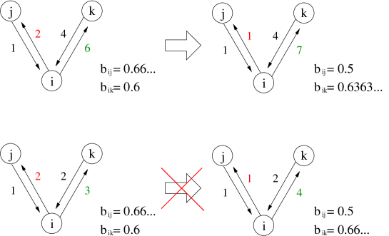
Unlike in the unweighted case, edge weights allow us to study reciprocity as a property of a single edge instead of the full network. To this end we define the edge bias between nodes $v_{i}$ and $v_{j}$ as

b_{ij}=\frac{w_{ij}}{w_{ij}+w_{ji}}.

The edge bias is the simplest possible measure for studying reciprocity. Note that because $b_{ij}+b_{ji}=1$ , the distribution of $b_{ij}$ for all edges in the network is symmetric around $0.5$ and therefore it suffices to study only the range $b_{ij}\in[0.5,\,1]$ .

2 Data

We study the reciprocity of communication in a mobile phone data set consisting of 350 million calls between 5.3 million customers made during a period of 18 weeks. Mobile phone calls provide an excellent proxy for studying this kind of reciprocity because phone calls are at the same time directed and undirected: The calls are directed because it is the caller who decides to make the call and invest his time (and often money) in that particular relationship, but since the conversation during the call is undirected, there is no immediate reason for the recipient to call back shortly after. Consider the difference to SMS messages or emails where a conversation means sending a sequence of reciprocated messages, making it more difficult to study reciprocity by simply counting the number of messages.

To remove possibly spurious contacts, i.e. those that are more likely to be chance encounters instead of true social relationships, we have preprocessed the data by removing all unidirectional edges. Thus the unweighted reciprocity according to the definition above would be $r=1$ , and therefore the methods for analyzing the reciprocity of unweighted, directed networks are not applicable.²²2To be exact, $r\approx 1$ because any communication, either SMS message or call, was sufficient to make an edge bidirectional, and thus there are some edges where only one person has made calls. The weight $w_{ij}$ is the total number of calls customer $v_{i}$ made to $v_{j}$ during the whole 18 week period.

Refer to caption — Figure 1: Total degree distribution of the mobile phone data set separately for prepaid and postpaid users. Inset: The distribution until $k=30$ in semi-logarithmic coordinates.

The customers can be split into two groups based on how they pay for their mobile phone service: prepaid users pay for their usage beforehand, postpaid users pay afterword. While this initial difference might seem small, it results in major differences in the basic statistics and it is therefore necessary to analyze the two user groups separately. The statistics of calls between prepaid and postpaid users would mostly just reflect the differences in degree and strength distributions (discussed below). Thus in this article we only study calls between pairs of prepaid users and calls between pairs of postpaid users. The two user groups are approximately equal in size.

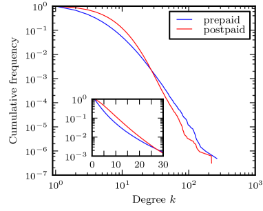
The basic statistics of the network often imprint also more complex statistics, and it is therefore a good idea to first go through some basic distributions. The degree $k_{i}$ of a node is defined as the number of neighboring nodes. Because all edges in our network are bidirectional after preprocessing, the out-degree (number of people called) always equals the in-degree (number of people from whom a call has been received). The degree distributions of the network, shown in Figure 1 separately for prepaid and postpaid users, have long power-law tails. The average degree was found to be 3.41 for prepaid users and 5.15 for postpaid users.

The strength of a node is defined as the sum of weights of adjacent edges. For a directed network we can define both the out-strength $s_{i}^{\textrm{out}}=\sum_{j}w_{ij}$ , which is the total number of calls made, and the in-strength $s_{i}^{\textrm{in}}=\sum_{j}w_{ji}$ , the total number of calls received. The strength distributions in Fig. 2 turned out also to be fat-tailed, and we can see that postpaid users make much more calls. In fact, postpaid users make on average 10 times more calls than prepaid users. We can also see that prepaid users receive more calls than they make, while the most active postpaid users make more calls than they receive.

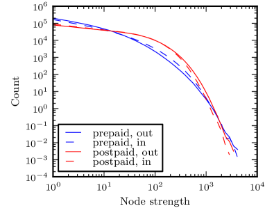
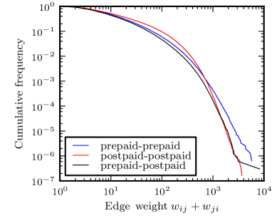
Figure 2 shows the total edge weight distribution for edges between users of the same or different type. There are more calls between users of the same type, which suggests that the user type is correlated between acquaintances.

The data set only includes the customers of a single mobile phone operator that has about 20 % market share in the country in question. While there are calls from and to people outside this customer base, this has no skewing effect on our study because our analysis concentrates on communication between the known customers, and this information is completely known.

3 Results

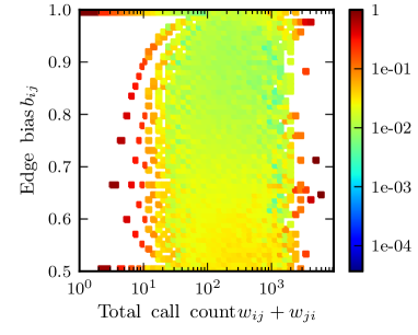
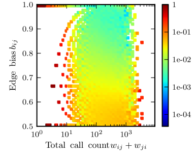
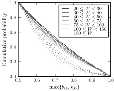
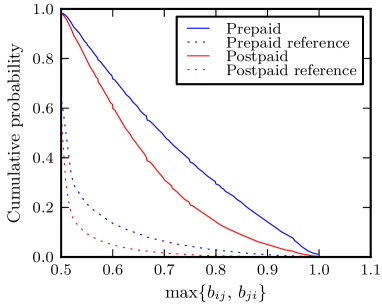
Figures 3(a) and 3(b) show the distribution of $b_{ij}$ for prepaid and postpaid users as a function of total edge weight. We can see that even though values around 0.5 are more common, there are still many edges with larger values of $b_{ij}$ . This becomes more obvious in Figure 4 that shows the cumulative distribution of edge bias for different weight ranges. For example among prepaid users the edges with $b_{ij}\geq 0.8$ , i.e. edges where one participant makes more than 80 % of all calls, make up over 25 % of all the edges even when the edge has over 100 calls. For postpaid users the numbers are somewhat smaller.

Naturally, we should not expect to find perfect reciprocity on all edges, but to justify treating social networks as undirected there should be some tendency towards $b_{ij}=0.5$ . But how much? The simplest step away from perfectly reciprocal relationships is to assume each dyad to be reciprocal in the probabilistic sense: both participants are equally likely to make a call. Thus, even though edges with only few calls could still be very biased, edges with 50 or more calls should have $b_{ij}$ very close to $0.5$ . This idea is also supported by Figure 4, where the distributions of high weight edges are somewhat more concentrated around $0.5$ .

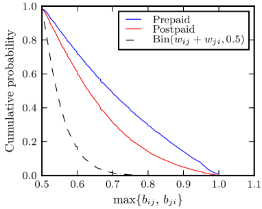
The hypothesis about equal likelihood for making a call implies that the edge bias values should follow a binomial distribution with $p=0.5$ and $n=w_{ij}+w_{ji}$ . However, Figure 4 shows that such a binomial distribution is far from truth: if the calls were evenly distributed between both participants, there should be almost no edges with $b_{ij}>0.7$ .

But is it reasonable to expect the edge bias values to be binomially distributed in the first place? As shown in Fig. 2, the node strengths vary widely, which itself might be enough to force large deviations from $b_{ij}=0.5$ — in other words the relationships would only appear biased because some people tend to call more than others. To test this claim we redistribute the total out-strength of each node onto its already existing edges so as to make the edge bias values as close to 0.5 as possible (see Appendix for details). It turns out that it is in fact possible to significantly reduce the number of high edge bias values, especially among postpaid users, as shown in Fig. 4. This proves that the strength distribution is not a sufficient explanation for the large edge bias values.

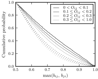
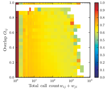
Since it appears that the edge bias cannot be explained away by properties of the node but is instead an intrinsic property of the edge itself, it is interesting to see whether it correlates with other local features of the network. Is there for example a connection between the edge bias and the community structure of the network? We measure local community structure with edge overlap, defined as $O_{ij}=n_{ij}/((k_{i}-1)+(k_{j}-1)-n_{ij})$ , where $n_{ij}$ is the number of common neighbors of nodes $v_{i}$ and $v_{j}$ . Thus the edge overlap gives the fraction of common neighbors out of all possible common neighbors, and is therefore larger in denser parts of the network.

Looking at Figure 4 it seems that the edge bias does indeed correlate with overlap: larger overlap implies an edge bias more concentrated around 0.5 for both prepaid and postpaid users. However, Figure 5 shows that the observed effect is in fact a spurious result of two other correlations. The first correlation is the one between edge bias and weight, shown in Fig. 4. The second correlation is the Granovetter hypothesis [12], which states that edges between communities should be weaker than those inside communities. It was shown in [2] that in a mobile phone network this is indeed the case: edge weights are higher in denser parts of the network.

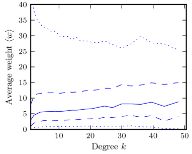
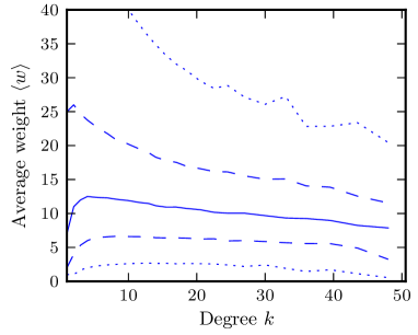
Finally, Figures 6(a) and 6(c) show that there is a connection between the edge bias and the degrees of the caller and the recipient. This simply confirms the everyday observation that people with many contacts tend to be active in keeping up those contacts, as opposed to simply waiting for the others to call them. While for prepaid users this observation results at least partly from the fact that average out-weight increases with degree (Fig. 6(b)), this is not the case with postpaid users. In fact, of the edges between two postpaid users the one with a larger degree is on average more active, even though the average edge weight decreases with degree (Fig. 6(d)).

4 Discussion

We have shown that highly biased edges where one participant is much more active than the other are abundant in a mobile phone network. Although the strength distribution can explain some of the observed high bias values, it is by no means a sufficient explanation.

Making a phone call is always an investment in a relationship: not only does it cost time and money to the caller, but the caller must also make a conscious decision to make the call. While people are in general known to strive to make their relationships reciprocal, we can observe plenty of relationships with a striking lack of reciprocity.

It was mentioned earlier that the fact that the data only includes 20 % of the population has no adverse effect on the data. This should now be quite obvious, since we have only looked at the edges of which we have full information. However, we can state something even stronger: it is likely that any additional data would only improve the reference calculated above, because there would be more edges to choose from during the optimization. This of course assumes that the edge bias on the missing edges is distributed similarly as in the current data, which we feel is a very reasonable assumption.

We have so far deferred the discussion about whether the results can be extended to human relations in general. There are obviously many factors that influence the reciprocity of a relationship, as is evident from the differences between prepaid and postpaid users. We note that these difference do not necessarily stem straight from the differences in paying. For example, since the prepaid service is used more often by young people, our findings suggest that the relations among young people are more biased. Obviously hypotheses like this one need more research until we can say anything conclusive.

Data sets including communication through several different channels, such as email, online chatting and real life conversations, would be especially well suited for studying reciprocity, but unfortunately such data sets are difficult to acquire in the large scale required. The methods used here can however be readily applied to any such data, as long as the data includes information on who initiated the communication.

Acknowledgment

This work is partially supported by the Academy of Finland, the Finnish Center of Excellence programme 2006–2011, proj. 129670. We would also like to thank prof. Albert-László Barabási of Northeastern University for providing us access to the unique mobile phone data set and continuing collaboration thereof.

References

[1] S. Goodreau, Advances in exponential random graph (p^∗) models applied to a large social network, Social Networks, 29 (2) (2007) 231–248.
[2] J.-P. Onnela, J. Saramäki, J. Hyvönen, G. Szabó, D. Lazer, K. Kaski, J. Kertész, and A. L. Barabási, Structure and tie strengths in mobile communication networks, PNAS 104 (18) (2007) 7332–7336.
[3] F. Liljeros, C.R. Edling, L.A. Amaral, E.H. Stanley, and Y. Aberg, The web of human sexual contacts, Nature 411 (6840) (2001) 907–908.
[4] P. Wang, M.C. Gonzalez, C.A. Hidalgo, and A.-L. Barabasi, Understanding the spreading patterns of mobile phone viruses, Science 324 (5930) (2009) 1071–1076.
[5] C. Hidalgo and C. Rodriguez-Sickert, The dynamics of a mobile phone network, Physica A 387 (12) (2008) 3017–3024.
[6] M.E.J. Newman, The structure of scientific collaboration networks, PNAS 98 (2) (2001) 404–409.
[7] P. Holme, Network reachability of real-world contact sequences, Phys. Rev. E 71 (4) (2005) 046119.
[8] S. Wasserman and K. Faust, Social Network Analysis: Methods and Applications, Cambridge University Press, 1994.
[9] M. E. J. Newman, S. Forrest, and J. Balthrop, Email networks and the spread of computer viruses, Phys. Rev. E 66 (3) (2002) 035101.
[10] D. Garlaschelli and M.I. Loffredo, Patterns of link reciprocity in directed networks, Phys. Rev. Lett. 93 (26) (2004) 268701.
[11] G.Z. López, V. Zlatić, C. Zhou, H. Štefančić, and J. Kurths, Reciprocity of networks with degree correlations and arbitrary degree sequences, Phys. Rev. E 77 (1) (2008) 016106.
[12] M.S. Granovetter, The strength of weak ties, The American Journal of Sociology 78 (6) (1973) 1360–1380.

Appendix

We constructed a reference network to find out how what portion of the high edge bias values can be explained by the out-strength distribution. Unlike in-strength, the out-strength can be seen to reflect the activity of each user, and is closely controlled by each individual. Thus is it feasible to think that each call made could have been directed to some other contact instead of the one actually called. We calculate the reference for the whole network, comprising both the prepaid and postpaid users, and only separate the users groups in the final reference network. This is based on the assumption that customers do not know or care about the user type (prepaid or postpaid) of the recipient of the call, and thus any call made to a user of one type could have been made to a user of the other type.

There are obviously many ways of pursuing the goal of a bias distribution centered around $b_{ij}=0.5$ . We decided to base our method on the reasonable hypothesis about binomial distribution of edge weights which was discussed in Section 3: we attempt to maximize the likelihood that the edge bias values come from binomial distribution with $p=0.5$ , that is, we try to find a new set of edge weights $\mathbf{w}=\{w_{ij}\}_{e_{ij}\in\mathbf{E}}$ such that

\begin{split}\mathbf{w}=\mathrm{arg}\max&\,\Pi_{(i,j)\in\mathbf{E}}\textrm{Pr}(w_{ij}\,|\,w_{ij}\sim\mathrm{Bin}(w_{ij}+w_{ji},\,0.5))\\ \mathrm{s.t.}&\sum_{j}w_{ij}=s_{i}~{}\forall v_{i}\in V,\end{split}

where $s_{i}$ is the out-strength of node $v_{i}$ in the original network. The topology of the original network is also preserved, which means that the edge set $\mathbf{E}$ remains the same during the optimization.

Taking a logarithm and writing the binomial probabilities explicitly, we get

\begin{split}\mathbf{w}&=\mathrm{arg}\max\sum_{e_{ij}\in\mathbf{E}}\log\frac{(w_{ij}+w_{ji})!}{w_{ij}!w_{ji}!}p^{w_{ij}}(1-p)^{w_{ji}}\\ &=\mathrm{arg}\max f(\mathbf{w}),\end{split}

where $f(\mathbf{w})$ is the global target function

f(\mathbf{w})=\sum_{e_{ij}\in\mathbf{E}}\Bigl{(}\sum_{u=1}^{w_{ij}+w_{ji}}\log u-\sum_{u=1}^{w_{ij}}\log u-\sum_{u=1}^{w_{ji}}\log u\Bigr{)}.

(1)

Finding the global optimum of this function is not straightforward, as it is likely to have several local optima. We carry out the optimization in two-phases. The first phase is simulated annealing, which aims at avoiding bad local optima. One step of the simulated annealing algorithm selects a random node $v_{i}$ and moves one unit of weight³³3Since the edge weights are in this case call counts, they are discrete and reasonably small. from edge $(v_{i},\,v_{j})$ to $(v_{i},\,v_{k})$ , where $v_{j}$ and $v_{k}$ are random neighbors of $v_{i}$ , with a probability proportional to the change of the target function $f(\mathbf{w})$ , given by

\begin{split}\Delta f(\mathbf{w})&=f(\mathbf{w};\,w_{ij}\mapsto w_{ij}-1,\,w_{ik}\mapsto w_{ik}+1)\\ &~{}~{}~{}-f(\mathbf{w})\\ &=\log\frac{w_{ij}(w_{ik}+w_{ki}+1)}{(w_{ij}+w_{ji})(w_{ik}+1)}=\log\frac{b_{ij}(0)}{b_{ik}(1)}.\end{split}

In the last step we have defined

b_{ij}(\delta)=\frac{w_{ij}+\delta}{w_{ij}+w_{ji}+\delta}

which is the bias of edge $(v_{i},\,v_{j})$ after adding weight $\delta$ . This final result is surprisingly simple: the target function value is increased whenever $b_{ij}(0)>b_{ik}(1)$ . Interestingly, while $f(\mathbf{w})$ was derived by maximizing the likelihood of binomial distributions, we end up comparing the edge biases. The two biases involved in the comparison implicitly account for the form of the binomial distribution; see Figure 7 for further clarification.

When the temperature of the simulated annealing becomes low, there is little or no randomness left, but the algorithm is still quite slow. We therefore use a greedy algorithm as the second phase of the optimization. The greedy algorithm starts from where the simulated annealing finished, and simply descends to the local optimum as efficiently as possible.

The greedy optimization goes through the nodes in a round-robin manner, but unlike simulated annealing, improves the target function by changing weights around one node until no further progress is possible. It works by selecting the two edges that give the maximum improvement of the target function, $j^{*}=\arg_{j}\max\{b_{ij}(0)\}$ and $k^{*}=\arg_{k}\min\{b_{ik}(1)|k\neq j^{*}\}$ , and changing $\delta^{*}=\left\lceil\frac{w_{ij}w_{ki}-w_{ji}w_{ik}-w_{ji}}{w_{ji}+w_{ki}}\right\rceil$ units of weight from edge $(v_{i},\,v_{j^{*}})$ to $(v_{i},\,v_{k^{*}})$ . $\delta^{*}$ is the largest amount of weight that still improves the target function, defined as the largest integer for which $b_{ij}(1-\delta)>b_{ik}(-\delta)$ is true. The optimum is reached when no change occurs during one round through all nodes.