Astrometric signal profile fitting for Gaia

Abstract

A tool for representation of the one-dimensional astrometric signal of Gaia is described and investigated in terms of fit discrepancy and astrometric performance with respect to number of parameters required. The proposed basis function is based on the aberration free response of the ideal telescope and its derivatives, weighted by the source spectral distribution. The influence of relative position of the detector pixel array with respect to the optical image is analysed, as well as the variation induced by the source spectral emission. The number of parameters required for micro-arcsec level consistency of the reconstructed function with the detected signal is found to be 11. Some considerations are devoted to the issue of calibration of the instrument response representation, taking into account the relevant aspects of source spectrum and focal plane sampling. Additional investigations and other applications are also suggested.

Introduction

In the framework of the data reduction for Gaia (Perryman, 2005; Lindegren, 2009), the issue of a convenient representation of the instrument response, i.e. of the detected signal profile, at the micro-arcsec (hereafter, $\mu as$) level, is crucial to science data modelling, calibration and analysis.

Since a large fraction of the astrometric data of Gaia is one-dimensional, obtained by across scan binning during the CCD readout with the purpose of reducing the sheer amount of data, the investigation and analysis is referred to single-valued functions of one variable, i.e. intensity vs. focal plane position. The signal coordinate is basically coincident with the high resolution direction of the telescope, and with the scanning direction of the satellite. The one-dimensional signal is referred to as Line Spread Function (LSF) in the following, for similarity with the optical signal of an infinite slit, although the term is only applicable in a loose sense: e.g., the signal from one source may suffer contamination by other sources at some distance in the across scan direction, which would not be the case for real LSFs. Also, the finite readout area implies a small variation of the detected photon fraction with the across scan position on the detector, which would not happen for an LSF of negligible across size.

The signal profile from a real instrument differs from the ideal telescope response because of optical aberrations, instrument operation, detector characteristics, and a number of environmental aspects influencing them; also, the signal depends on the individual source spectrum. The detected signal can evolve during the mission lifetime due to degradation of both optical and electronic components. In the analysis described in this document, the case of comparably small perturbation to the ideal image, represented by small optical aberrations, is dealt with; the signal model can be extended to larger image degradation with straightforward modifications, but the precision can be expected to suffer progressive degradation as well. The modeling precision could then be retained by a description based on a larger number of parameters.

The proposed modeling framework is based on a set of functions, described in Sec. 1, derived from the monochromatic, aberration free LSF of an idealised telescope retaining the basic geometric characteristics of the Gaia instrument, i.e. the rectangular aperture width $L_{\xi}=1.45\,m$. The source spectrum is explicitly inserted in the construction of the polychromatic LSF, again referred to the aberration free telescope. Some of the additional image degradation effects associated with detector characteristics and operation are then introduced (Sec. 1.2). The signal degradation effects associated to a realistic instrument and operation, including known effects not explicitly included in the model, are then described by the expansion of individual signals in terms of the proposed function set.

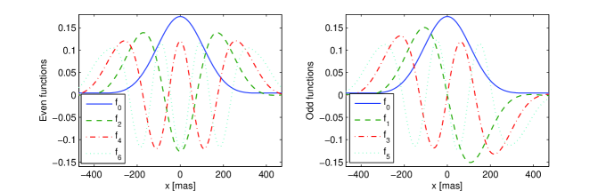
Figure 1: Polychromatic basis functions for a 6000 K source: even terms (left) and odd terms (right)

The implications of the proposed model are evaluated in Sec. 2 by simulation over a range of aberrations, of sampling offset (meaning the relative position of the optical image vs. the detector pixel array), and of source spectral type, modeled as blackbodies at different effective temperatures. The simulation is implemented in the Matlab framework. Remark: it is assumed that variation of relevant system parameters (e.g. detector electro-optical characteristics) can be represented, at first order, by optical aberrations inducing a similar effect on the detected signal.

The number of parameters required for proper fit of the detected signal with adequate precision are derived, and some of the mathematical and physical characteristics are discussed. In Sec. 3 the calibration of the model parameters is addressed with respect to some measurement aspects. In Sec. 4 we discuss some of the possible developments related to the proposed model, in terms of improvement of its performance and generality, as well as usage in other cases, like the photometric and spectroscopic instruments of Gaia, or other astronomical equipment. Finally, we draw our conclusions on the effectiveness of the proposed signal expansion model.

1 Signal model

The starting point of our derivation is the monochromatic response of an ideal instrument, i.e. the signal generated by an infinite slit, without aberrations. This is the well known squared sinc function, hereafter called parent function (Born & Wolf, 1999), depending on an adimensional argument related to the focal plane coordinate $x$, the wavelength $\lambda$ and the aperture width $L_{\xi}$, as

$$f_{0}^{m}\left(x\right)=\left[\frac{\sin\rho}{\rho}\right]^{2},\;\rho=\pi\frac{xL_{\xi}}{\lambda F}\,.$$ (1)

Many function families known in mathematics are solutions to differential equations, are derived from recurrence relations, or from a generating function. In our case, since there are no clear constraints of this kind, we decided to adopt a very simple construction rule. Additional functions are generated by the parent function derivatives, as

$$f_{n}^{m}\left(x\right)=\frac{d}{dx}f_{n-1}^{m}\left(x\right)=\left(\frac{d}{dx}\right)^{n}f_{0}^{m}\left(x\right)\,.$$ (2)

The overall set of functions will be addressed in the following as “basis functions”, although a rigorous mathematical framework supporting the term will not be implemented. It is thus considered as just an expedient naming convention.

In the following, the focal plane units will either be micrometers ($\mu m$), pixels (1 pixel = 10 $\mu m$), or milli-arcsec (mas), taking into account the Gaia aperture $L_{\xi}=1.45\,m$, the effective focal length of the telescope ($EFL=35\,m$) and the corresponding optical plate scale ($s=5.89\,arcsec/mm$).

The rationale leading us to test this particular approach is that the signals of interest are expected to be reasonably close to the ideal case, i.e. that they fit a context of small perturbation / small aberration. Therefore, an expansion in terms of the aberration free signal and related functions appears to be a promising tool. Notably, even in case of large aberrations, as images for conventional ground-based telescopes, the individual speckles are still described by a superposition of displaced copies of the aberration free telescope response, and the seeing image derives from integration of subsequent speckles. The parent function takes advantage of one of the basic aspects of the Gaia instrument, i.e. the telescope pupil size in the main measurement direction (hereafter also high resolution or along scan direction). Other basic factors of the instrument geometry, characteristics and operation may be included in the basis functions, as described below.

One peculiar aspect of the investigated basis functions is that they are all referred, by construction, to a common “zero point” of the coordinates, corresponding (as centre of the aberration free image) to the ideal position of the source image as provided by the geometric optics. Also, they have simple symmetry: odd numbered functions, as odd order derivatives of the even parent function, are odd, whereas even numbered functions are even. In the numerical implementation, since standard Matlab arrays or matrices are numbered from one onward, the parity and function numbering are exchanged, i.e. the parent function is term no. 1, and so on. The lowest order polychromatic functions, including the detection effects, are shown in Fig. 1.

1.1 Polychromatic basis functions

For any wavelength and position, it is possible to compute the monochromatic basis functions above. The parent function is defined by the geometry of the ideal instrument; it can be computed, with its derivatives, in either numerical or analytical form, using the trigonometry related expressions from 1, or the corresponding power series expansion.

The superposition of monochromatic LSF terms at different wavelength is weighted by the source spectral distribution, composed with the instrument transmission distribution and the detector response curve. The monochromatic basis is, by construction, source independent; the polychromatic LSF construction factors out explicitly the contributions from astrophysics (source spectrum) and astronomy (e.g. reddening). The polychromatic LSF, and its derivatives, labelled as $\{f_{0},\ldots,f_{N}\}$, must be computed numerically because of the arbitrary weighting function corresponding to the effective spectrum $S(\lambda)$. The polychromatic parent function can thus be expressed as

$$f_{o}(x)=\int d\lambda\,S(\lambda)\cdot f_{0}(x;\lambda)\,,$$ (3)

where the wavelength dependence of the monochromatic parent function is explicited in Eq. 1. The construction of additional basis functions is straightforward, as from Eq. 2.

We adopt a simple blackbody model for the source spectrum, which is not a detailed representation of many astrophysical objects, but is adequate to cover a realistic range of stars with respect to broadband imaging; a representation of the Gaia spectral response and of the normalised blackbody curves for three source temperatures is shown in Fig. 2.

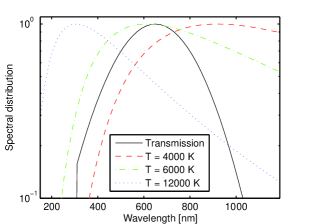
Figure 2: Spectral distributions of blackbodies at different temperatures superposed to the astrometric instrument response

1.2 Detection effects

Additional modifications to the signal profile are induced by other known parts of the detection process, in particular the geometric effects of finite pixels, inducing a smoothing of the optical profile through a rectangular filter with width corresponding to the pixel size; the detector Modulation Transfer Function (MTF); the dynamical mismatch between optical image and pixel array due to the Time Delay Integration (TDI) operation. Some of the effects of finite sampling and pixel size have been discussed, also in terms of the location algorithm performance, in Gai et al. (1998). In the current simulation, such contributions have been introduced as a wavelength independent signal smoothing with realistic equivalent length, respectively $10\,\mu m$ (geometric pixel size); $5\,\mu m$ (MTF); $5.1\,\mu m$ (TDI). A more realistic wavelength dependent description might in future be introduced e.g. for the MTF.

The superposition of wavelength contributions tends to average out the function oscillations at increasing distance from the central point. A sort of “ortho-normalisation” (depending on the current sampling, i.e. offset) is applied, so that the integral of the product of two basis function $f_{p},\,f_{q}$, over the detection interval $\{x_{m}\}$, vanishes for different terms and is unity for the “diagonal” term $p=q$: $\sum_{m}f_{p}\left(x_{m}\right)f_{q}\left(x_{m}\right)=\delta_{pq}$, using the Kronecker’s $\delta$ notation. An example of the resulting set of functions is shown in Fig. 1 for a $T_{s}=6000\,K$ source.

Remark: only the symmetric detection effects (pixel geometry, MTF and TDI) have been included in the template, in order to preserve the function symmetry. The simulated signals can include any kind of degradation effect, which will appear in terms of distribution of the fit coefficients.

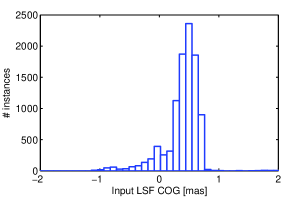
Figure 3: Histogram of the detected photo-centre values over the data set, zero detector offset

2 Simulation

The goal of the fitting process is to reproduce the aspects of interest of the measured signal $l(x_{k})$, corresponding to the LSF generated by the optical system and detected by the CCD. The sampled LSF is computed on a set of pixel centre positions $x_{k}$, with $1\,\mu m$ resolution, i.e. 1/10 pixel, thus providing a high resolution representation of the actual signal expected in operation. The detected LSF $l$ is then fed to the fitting algorithm, deriving the coefficients $c_{n}$ of a linear expansion referred to the basis functions centred in a convenient location $\tilde{x}$:

$$l(x_{k})=\sum_{n=1}^{N}c_{n}\cdot f_{n}(x_{k}-\widetilde{x})\,,$$ (4)

where the equality is intended in the least square sense. The fit quality can be evaluated in terms of consistency with the input data, e.g. based on three criteria:

• root mean square (RMS) discrepancy;

• integral difference (photometry);

• photocentre difference (astrometry).

The first two items are strictly related, since two functions with negligible RMS difference also have, at first order and under reasonable assumptions, the same integral. Hereafter, the results will be discussed based on the RMS discrepancy and photocentre difference only, using for the latter the model independent barycentre or centre of gravity (COG) algorithm. The COG is very simple, but in many respects not practical for the Gaia data reduction with respect to both random and systematic errors(Lindegren, 1978).

It is assumed that a good fit, reproducing the input data profile and position (with a given location algorithm), will also provide consistent estimates of other parameters of interest, whichever the selected algorithm. Verification of performance and robustness of specific algorithms should be considered in practical cases.

The sample set for the main simulation includes 10000 different instances of optical aberrations, generated by a random set of coefficients for the Legendre polynomials of order up to 5 and 15, respectively on the short (across scan) and long (along scan) side of the main telescope aperture (respectively $0.5\times 1.45\,m$), providing a representation of wavefront error (WFE) down to the $0.1\,m$ scale. Below, different signal instances are sometimes referred to by the RMS WFE, i.e. the RMS value of the WFE over the telescope pupil; the aberration free image has zero RMS WFE. The pupil is sampled with resolution $1\,cm$ in both directions. The focal plane image resolution is $1\,\mu m$ and $3\,\mu m$ respectively in the along and across direction, corresponding in both cases to 1/10 of the geometric pixel size. The spectral resolution is 20 nm, in the wavelength range 300 to 1100 nm; a realistic transmission curve is implemented by a Gaussian distribution with $\sigma=250\,nm$ and peak at 650 nm. The focal plane image is built by numerical computation of the diffraction integral, according to the prescriptions in Gai & Cancelliere (2007), and integrated in the low resolution direction to represent the operating mode of Gaia over a large fraction of the science data. The LSF is computed with $1\,\mu m$ resolution over a region of $150\,\mu m$ (15 pixels), and the detection effects are included, as for the basis functions. Representative readout samples corresponding to 12 pixels (following nominal Gaia operation for intermediate magnitude objects), with selected offset and $1\,\mu m$ resolution, are then used in the fitting process described below.

For each instance, a different WFE and source temperature is used, to cover a realistic range of variation of instrument parameters and observed target. The source is represented by a simple blackbody distribution, filtered by the instrument throughput (Fig. 2). In practical applications, realistic spectra can be inserted e.g. by means of data tables (relative intensity vs. wavelength) or other convenient descriptions.

Remark: the nominal instrument configuration is associated to a limited range of variation of the aberration coefficients describing the change in optical response over the limited region of the focal plane used by the detector. The simulation adopts a wide range of aberration coefficients in order to cover not only the nominal values of the relevant parameters of the optical configuration and of the detector electro-optical characteristics, but also realistic modifications of the in-flight system due to the transfer from ground to orbit and consequent re-alignment. Also, limited degradation of such parameters during operation, e.g. related to ageing or radiation damage, modifying the detected signal profile, can described up to a point by an appropriate change in the aberration coefficients.

Therefore, our investigation provides indications on the capability of the proposed fitting approach to follow the instrument response evolution, of course by update of the coefficients through a convenient calibration procedure. It is assumed that the system remains stable over time periods sufficient for determination of the describing parameters with sufficient precision and reliability.

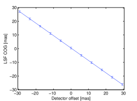
Figure 4: Average COG vs. offset, with RMS spread shown as an error bar

The distribution of aberration instances generates a range of photocentre values, evaluated on the zero offset sampled LSF by the COG algorithm, and shown in Fig. 3. Notably, the typical photocentre displacement is below $1\,mas$, i.e. small with respect to the RMS size of the LSF ($\sim 130\,mas$), but significantly larger than the measurement precision goal for intermediate magnitude stars (order of $0.1\,mas$ at the elementary exposure level, and order of $10\,\mu as$ for the final catalogue). The spread in values associated to the statistical sample has mean 0.446 mas, and RMS 0.619 mas. In this case, the optical image is set with the coordinate origin coincident with the centre of the detector pixel array, so that the aberration free image is centred. The COG variation is due to distortion (in the strictly optical sense) and to all other aberrations and degradation effects inducing modifications in the signal profile, i.e. both actual translations and deformations. Since the signal is sampled over a finite region of the focal plane, the different truncation of an asymmetric, displaced distribution affects both the photocentre and the fraction of energy actually detected, i.e. the photometry.

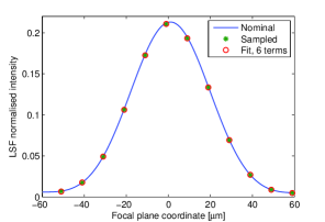
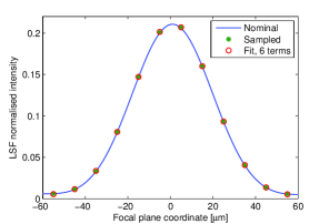
Figure 5: Example of 12 pixel sampled LSF (crosses) and its fit to 6 terms (circles), on top of the 1 $\mu m$ resolution LSF (solid line), for offset zero (left) and 0.4 pixels (right); the detected signal, i.e. relative pixel intensity, is a function of the sampling offset

Throughout the simulation, we apply a set of offsets to the LSF sampling process, to represent a realistic range of displacement between the optical image and the detector. A displacement larger than 0.5 pixel just means that a different central pixel should be selected. The range $\pm 0.5$ pixel is covered with resolution 0.1 pixel. The overall distribution of the sampled LSF COG, for all cases of offset, is shown in Fig. 4, evidencing that the COG spread remains small for any applied offset, confirming that the selected readout window is not affected by large signal variations. The COG estimated on the detected image seems therefore to be a reasonable first approximation for estimation of the detector offset, or correspondingly for the actual image position vs. the detector considered as a reference, and as such it will be used in the following steps of the simulation.

Notably, the correlation between detector offset and average COG, shown in Fig. 4 (the error bars are the RMS values of the COG distribution for each offset), is negative, since a given offset applied to the detector corresponds to an image displacement in the opposite direction. The estimated COG is not equal (in absolute value) to the detector offset, because the LSF sampling positions change: one of the LSF wings is pushed inside the sampling region, the other outside, thus inducing a residual COG displacement. Typical residual values are below 10% of the applied offset, and comparable with the COG spread among different LSF instances, so that the COG of sampled data provides a reasonable estimate of the mismatch between LSF location and pixel array, and might be used as starting approximation for more advanced algorithms.

2.1 Astrometric and photometric fit

For any WFE case, a set of offset values is introduced between the pixel array and the sampling positions of the LSF, in the range $\pm 0.5$ pixel, with resolution 0.1 pixel. The signal range corresponds to the 12 sample readout region, but with $1\,\mu m$ resolution, i.e. for the zero offset case the sampling positions are $[-55;\,-54;\,-53;\,\ldots;\,53;\,54;\,55]\,\mu m$. The 110 points signal avoids any risk of fit degeneration using up to 11 terms. The offset cases correspond to displaced sampling positions by $[\pm 1;\,\pm 2;\,\pm 3;\,\pm 4;\,\pm 5]\,\mu m$. The COG of the offset, sampled LSF is selected as reference point (origin) of the basis functions used for signal fitting. In Fig. 5, a selected LSF instance (nr. 1) is shown, superposed to the 12 sample LSF expected in operation (crosses) and to the corresponding fit result using 6 terms from the basis function set (circles), respectively for offset zero (left panel) and 0.4 pixel (right panel); the fitting error is barely perceivable on this scale on the sides of the central lobe.

The best fit is computed against an increasing number of basis function terms, to evaluate the most convenient number of terms required for proper description of the sampled data derived from the input LSF. The fit performance is then discussed.

2.1.1 Fit residuals vs. offset

The RMS fit discrepancy for a few offset cases are shown in Fig. 6, as a function of increasing number of fitting terms. In particular, the left panel shows the average over the sample (i.e. for different aberrations) of the RMS discrepancy between the sampled LSF and the fit, as a function of the number of basis functions used for the detected signal expansion. The RMS over the sample is shown on the right.

The fit retrieves most of the input signal with 10 to 11 terms, according to the progressively decreasing RMS over the data set of the residuals with increasing number of fitting terms, describing an increasing capability of the fit in capturing the fine details of the LSF. The 11 terms case evidences that the fit is not exact, but it provides a dramatic improvement with respect to lower dimensionality cases.

Using one or two terms, the fit already accounts for more than 99% of the LSF energy, and with three or four terms the RMS discrepancy decreases to about $10^{-4}$. Using five to eight terms, the RMS discrepancy further drops to the $10^{-5}$ level, dropping to the $10^{-6}$ level with 11 terms.

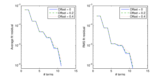
Figure 6: Fit discrepancy RMS vs. number of terms up to 11, zero offset; average (left) and RMS (right) over the data set

The fit RMS discrepancy can be evaluated as a function of the offset between LSF and pixel array, and the results for 10 (left) and 11 (right) fitting terms are summarised in Fig. 7, where it appears that the residuals increase with the absolute value of offset, are affected by a significant variation over the LSF sample, and improve by a factor four by switching from 10 terms (average $\sim 8\times 10^{-6}$) to 11 terms (average $\sim 2\times 10^{-6}$).

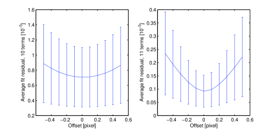
Figure 7: Fit discrepancy mean and RMS (as error bar) vs. offset, using 10 (left) and 11 (right) terms

Therefore, photometry and the image profile are basically retrieved by modeling the LSF with either 10 or 11 terms of the proposed basis functions. This result is not yet conclusive, since the crucial parameter under investigation is the astrometric performance, dealt with in the next section.

2.1.2 Astrometric residuals vs. offset

Concerning the astrometric precision of the fit, Fig. 8 shows that, for the range 8 to 11 fitting terms, the COG of the reconstructed LSF converges to the COG of the input sampled LSF, both as mean value (left panel) and as RMS (right panel) over the data set, at increasing number of terms. This is consistent with the results of the previous section.

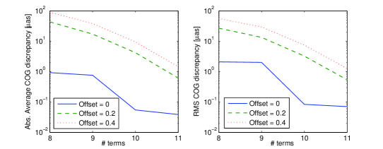
Figure 8: COG discrepancy vs. number of terms from 8 to 11 for three cases of offset: absolute mean value (left) and RMS (right) over the data set

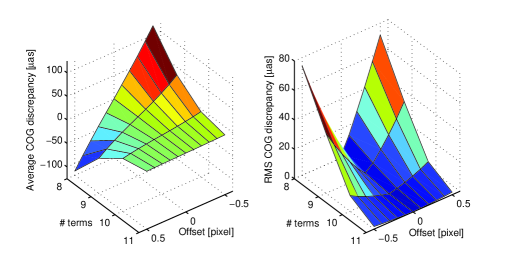
Figure 9: COG discrepancy vs. number of fitting functions and offset, mean (left) and RMS (right) values

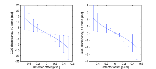
Figure 10: Mean COG discrepancy vs. offset, for 10 (left) and 11 (right) fitting terms; RMS discrepancy shown as an error bar

A COG error of few $\mu as$ RMS, around a comparable average error, is achieved for the zero offset case with 8 terms. For larger offset values, the discrepancy grows steeply, requiring either 10 or 11 terms to retrieve $\mu as$ precision. The COG precision is shown as a function of the selected number of fitting terms and of the offset between LSF and pixel array in Fig. 9, as average (left panel) and RMS (right panel) distributions. The discrepancy is larger at increasing offset, and decreases with increasing number of terms. Although most offset cases are associated to larger RMS COG discrepancy than the zero offset, for a given number of basis functions, convergence to the $\mu as$ level is still achieved when 11 terms are used.

The COG discrepancy is shown in Fig. 10 respectively for the case of 10 (left) and 11 (right) fitting terms, plotting the mean value with a solid line and evidencing the RMS as an error bar. The mean COG discrepancy remains within $1\sigma$ from the desired zero value corresponding to unbiased signal reconstruction, but an overall trend of the bias as a function of the pixel offset is present.
We remark the dramatic improvement introduced by usage of 11 terms rather than 10 or less, reducing the RMS and average COG discrepancy from 15 $\mu as$ to 2 $\mu as$ peak, or from 7 $\mu as$ to 1 $\mu as$ on average vs. pixel offset. The scaling of centering residual is different from that of fit discrepancy (Fig. 7) because the location process is mostly sensitive to the steepest slope regions of the signal, thus affecting the error propagation (Gai et al., 1998).

2.1.3 Distribution of the fit coefficients

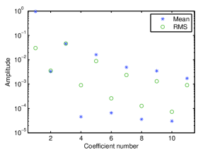
Figure 11: Fit coefficients for the zero offset case; mean (stars) and RMS (circles) over the data set

The relative weight of the fit coefficients, up to 11 terms, for the zero offset case is shown in Fig. 11, as statistics over the data set.

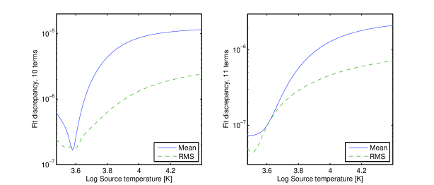
Figure 12: Fit discrepancy vs. source temperature, 10 (left) and 11 (right) terms, zero offset; mean (solid line) and RMS (dashed line) over the data set

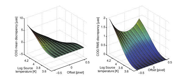
Figure 13: Average (left) and RMS (right) COG discrepancy vs. source temperature and offset, 11 terms

The average (stars) is close to zero for even terms (associated to odd functions), consistently with the expectations for averaging over a representative random distribution of aberrations. The RMS of the coefficients over the data set (circles) evidences that their spread is also very small, i.e. that the individual values are actually close to zero. The mean and RMS values for odd terms (even functions) decrease for increasing order of the functions. This is consistent with the simulation design of small aberration images, with deviations from the diffraction limit mostly due to symmetric degradation effects (pixel geometry, MTF, TDI).

2.2 Source temperature dependence

The fit quality is evaluated as a function of the source spectrum by generating a data sample, for a limited number of WFE instances (100), with blackbody source temperature spread uniformly, in logarithmic units, between 3000 K and 25000 K. The sample has thus 10000 instances, as in the simulation in Sec. 2.1, but the optical response variation is smaller, whereas the spectral coverage is finer. The sample is then processed similarly to the case described in Sec. 2.1, limited to 10 and 11 fitting terms, over a range $\pm 0.5$ pixel, always with resolution 0.1 pixel ($1\,\mu m$).

The zero offset case is first evaluated. The average fit discrepancy remains consistent with the previous results, as shown in Fig. 12, where the average (solid line) and RMS (dashed line) discrepancy are shown in logarithmic units vs. the source temperature. The spread is associated to the different aberration instances. Using 10 terms, the average discrepancy is below $10^{-6}$ for near-solar and later spectral types, and it increases for earlier types to $\sim 10^{-5}$. A similar trend is achieved for the 11 term case (right panel), with values reduced by roughly a factor five.

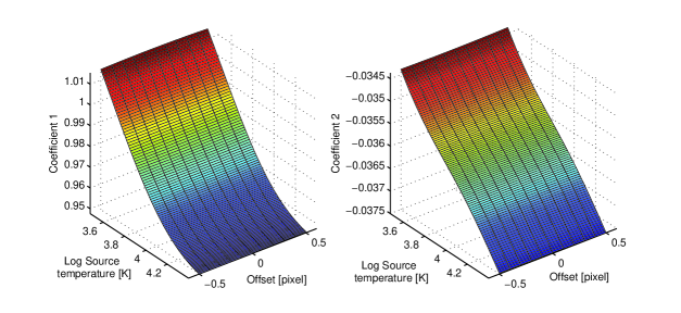
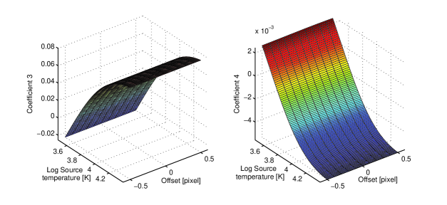
Figure 14: Fit coefficients 1 to 4 vs. offset and source temperature, WFE instance 1

The dependence of astrometric discrepancy from offset can then be considered. The average and RMS values vs. source temperature and offset, 11 terms, are shown in Fig. 13, left and right panel respectively. The average discrepancy reaches few $\mu as$ peak values, whereas the RMS remains below $2\,\mu as$ peak; the fit discrepancy is below $1\,\mu as$ for low temperature cases. Using 10 terms, the discrepancy is somewhat degraded, respectively to a few $\mu as$ RMS and a few 10 $\mu as$ on average over the data set. The error increase with the source temperature, being very small for near solar and later spectral types, will be further discussed in Sec. 3.
The variation of the fit coefficients 1 to 4 for the WFE instance no. 1, with both source temperature and offset, is shown in Fig. 14.

The variation of the fit coefficients over the data set depends on both source spectral characteristics (e.g. the source temperature or its logarithm, in the simple blackbody model) and sampling offset. The dependence is very smooth, as for the COG discrepancy (Fig. 13), so that is appears that it could be expanded in the form of a very simple function, e.g. low order polynomials. Besides, different instances of aberrated images exhibit, as could have been expected, different spectral dependence (Busonero et al., 2006). Therefore, it appears that the coefficients may be mapped over the field of view by calibration with comparable ease.

2.3 Sensitivity to source temperature

In the simulation described in Sec. 2.1, the random variation of both aberration and source temperature does not allow to evidence simple trends as those shown in Sec. 2.2. Besides, the simple dependence on source temperature evidenced in Sec. 2.2 suggests to investigate directly on this data set the sensitivity to errors in the knowledge of the source temperature. The same input data is used, again with $1\,\mu m$ resolution and ranging over $\pm 0.5$ pixel offsets; however, in the current run, a $\pm 1\%$ error on the source temperature is applied in the construction of the basis functions, thus representing an uncertainty on the knowledge of the source temperature or a spectral distribution variation either in the source itself (e.g. in case of a variable star) or in the instrument response. The fit is performed using both 10 and 11 terms.

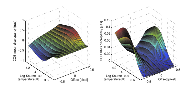
Figure 15: Mean (left) and RMS (right) COG discrepancy vs. offset and source temperature, with temperature error, 10 terms

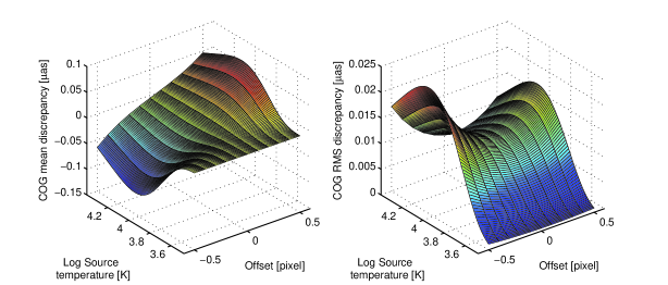
Figure 16: Mean (left) and RMS (right) COG discrepancy vs. offset and source temperature, with temperature error, 11 terms

The COG estimates for both $+1\%$ and $-1\%$ source temperature errors are then compared in order to assess the consequences on the measurements.

The COG difference between the two cases is shown vs. offset and temperature in Figs. 15 and 16, respectively for the case of 10 and 11 fitting terms, evidencing the mean (left) and RMS (right) values over the data set. The COG difference of either $+1\%$ or $-1\%$ error from the nominal source temperature COG result is smaller (about half as much). Over a 2% variation of the source temperature, using 10 terms, the mean COG discrepancy remains below $1\,\mu as$, with values much smaller for either low source temperature or small offset, and some mitigation also for very high temperature values. Correspondingly, the RMS COG discrepancy between the two cases is below $0.1\,\mu as$, with peaks corresponding to intermediate temperatures and large offset. Using 11 basis functions, the COG discrepancy is reduced by nearly one order of magnitude both in terms of mean and RMS values.

The astrometric error introduced by a $\pm 1\%$ error on the knowledge of the source temperature, therefore, induces a marginal variation ($\sim 1\%$) in the photocentre reconstruction, as seen e.g. by comparison with Fig. 13 or Fig. 10.

Since the fit error is very small, in spite of the temperature error, the sensitivity to knowledge of the source temperature, or to related variations, is small, even for the 10 term case. Assuming linear scaling, a 10% error on the source temperature will remain acceptable to a measurement accuracy of few $\mu as$ for most cases of optical response, using either 10 or 11 terms for the fit. Additional simulations may be required to provide better quantitative estimates of the sensitivity, due to the limited number of aberration instances, and model limitations at the sub-$\mu as$ level.

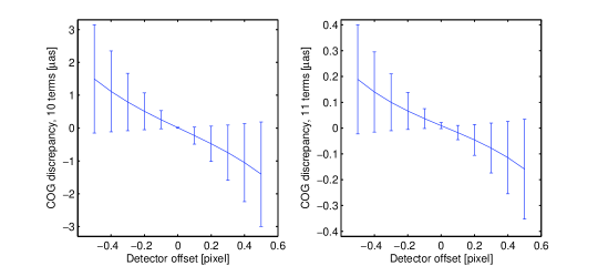
Figure 17: Mean COG discrepancy vs. offset (RMS as error bar), for 10 (left) and 11 (right) fitting terms, for instances associated to source temperature below 6500 K

3 Calibration aspects

The fit test discussed in Sec. 2.1 is somewhat artificial, since it is not applicable directly to science data due to simulation dependence on

1. pixel level sampling of real data, i.e. 10 $\mu m$ resolution rather than 1 $\mu m$;

2. pixel offset, i.e. relative phase between the currently observed target and the pixel array;

3. source spectral distribution;

4. photon limited information on individual exposures.

Actually, a model of the effective LSF should be derived from a set of data corresponding to several objects observed at different pixel offsets, as provided naturally by the spread of star positions on the sky. This procedure must also account for the variation of the coefficients with the source spectral characteristics; the composition of data also improves on the photon limit issue. It is necessary to feed the fit with a sufficiently large astrophysical sample, since individual exposure data are to be weighted according to their statistical significance, i.e. SNR and source brightness. The most convenient approach for practical implementation in the Gaia data reduction system should be further investigated. The above simulation approach was adopted for its simplicity, and is deemed adequate for a first assessment of the relevant properties of the proposed model, but it does not meet per se all needs for implementation in the data reduction pipeline.

The offset cases are not representative of the complete LSF reconstruction process: they relate to the case of individual observations, with the aim of identifying potentially relevant contributions to the systematic error. A few instances of bright, hot objects, detected with large offset, might introduce a comparably large bias in the reconstructed LSF, significant with respect to their photon limited location precision. The simulation results suggest that the data reduction system should monitor the LSF reconstruction against this situation, possibly introducing corrections. Still, usage of enough terms in the LSF modelling (up to 11) significantly reduces the individual bias contribution.

As an idealised case of real data composition, we assume that a large number of single exposure data are collated to cover the whole offset range and used to fit a single, zero offset LSF model; the sampling positions are then set to $[-60;\,-59;\,-58;\,\ldots;\,58;\,59;\,60]\,\mu m$, corresponding to 12 pixels (the readout region) $\pm 0.5$ pixels to account for the offset due to individual object positions. The issue of correct photocentre determination is neglected at the moment, as well as possible weighting based on offset, SNR and colour. The astrometric discrepancy vs. number of fitting terms of such high resolution LSF model with respect to the parent data set is shown in Fig. 18. The fit quality is at the $\mu as$ level RMS with 10 terms, and the mean value is somewhat lower; in practical cases, this suggests that the fit is expected to have negligible systematic error and noise dominated by the available amount of photon limited exposures.

The relevance of offset between optical image and detector may be better appreciated in terms of the equivalent total distortion, considered as the overall set of optical effects inducing image displacement. From the point of view of signal profile fitting, the applied displacement up to $\pm 0.5$ pixel, i.e. $\pm 29\,mas$, corresponds to about $\pm 1/6$ of the Airy diameter at $\lambda=600\,nm$ (about $30\,\mu m$, or 171 mas). Therefore, it is larger than the overall optical aberration introduced in the simulation sample, with average value of the RMS WFE below $\lambda/10$, and much larger than the astrometric effect induced on the images, below $\lambda/100$ (Fig. 3).

As shown in Sec. 2.2, in case of sources with simple spectral distribution, known with an acceptable tolerance (Sec. 2.3), a “grid” of calibration instances covering e.g. 10 to 20 different temperatures over the desired range, and order of 10 different offsets on the detector, is expected to provide satisfactory results. Besides, simple SNR considerations lead to the need of averaging many individual measurements in order to achieve photon driven precision comparable with the desired fit precision. For example, setting a goal of $10^{-5}$ on the RMS fit discrepancy corresponds to a requirement on the required cumulative SNR $\sim 10^{5}$, independent of the selected LSF expansion strategy. This corresponds to matching the fit precision associated to a given number of terms with the photon limit on the knowledge of the effective signal profile. Therefore, a 10 term fitting model, with lower intrinsic precision ($10^{-5}$), has more relaxed calibration requirements, since it is much easier (or faster) to accumulate the corresponding amount of photon limited data ($SNR\simeq 10^{5}$). Model monitoring procedures at the $10^{-5}$ level can then be applied on a time scale (i.e. data amounts) shorter by a factor 100 with respect to similar procedures aimed at the $10^{-6}$ precision goal, roughly corresponding to 11 fitting terms.

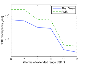
Figure 18: Extended range LSF model: astrometric discrepancy as a function of the number of fitting terms over $\pm 60\,\mu m$

Also, taking advantage of the fit quality vs. source temperature (Figs. 12 and 13), it might be found convenient to split the model into a part referred to near solar type objects, and a part with additional chromatic corrections for other objects. For example, using the data from Sec. 2.1 and restricting the data to lower source temperature ($T_{s}<6500\,K$), corresponding to about 3000 instances over 10000, the distribution of COG discrepancy vs. offset is shown in Fig. 17. By comparison with the corresponding Fig. 10, referred to the whole data set, a precision improvement by about one order of magnitude is achieved for both cases of either 10 (left) and 11 (right) fitting terms. In this case, $\mu as$ level precision is achieved already with 10 terms.

The better fit quality for near-solar spectral types can be related to the selected spectral passband of Gaia (Fig. 2), which collects a significant fraction of their blackbody distribution and includes their maximum. Warmer stars have a large fraction of their blackbody distribution outside the Gaia observing band, so that a comparably small change in the source temperature induces a significant displacement in the detected spectrum and its effective wavelength. A similar consideration holds for colder stars as well, but the image is in any case less affected by aberrations at longer wavelengths, due to the WFE scaling in the diffraction integral as $WFE/\lambda$.

4 Discussion

The simulation of Sec. 2.1 adopts a fitting strategy in which the basis function center is initially set to the sampled LSF COG, and never modified; only the function coefficients are adjusted to achieve the best fit, in the least square sense, with the input data. Since the goal is an LSF model reproducing both data profile and location, the correct approach would require that, for a selected number $N$ of fitting terms, a complete set of $N+1$ parameters were estimated for best fit with the data, i.e. the $N$ function coefficients and the additional term defining the new location estimate. Therefore, the fitting and location algorithms become entangled.

Moreover, due to the form of the basis functions, the model is no longer linear in its parameters, and the conventional least square approach cannot be considered to be mathematically correct. However, due to the assumptions of small deviations from the aberration free signal, the correlation between photocentre and fit coefficients may be comparably loose, and an iterative solution can be expected to converge for all parameters. In particular, the function coefficients could be approximated by setting the initial values as $c_{0}=1$; $c_{2}=\ldots=c_{N}=0$.

This approach was not investigated in this stage of development, under the assumption that the simplest, location independent fitting algorithm already provides sufficient indications on the achievable fitting performance of the proposed model. The fit convergence in terms of rapidly diminishing values of both RMS discrepancy and COG difference seems to confirm the soundness of the proposed strategy. More complex fitting approaches will be considered in future investigations.

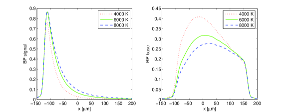
Figure 19: Parent function for the BP (left) and RP (right) instruments for different source temperatures

The model fitting was implemented over a limited readout region (12 pixels) to match the nominal Gaia operation on intermediate brightness objects; the extension to faint objects, on which a lower number of readout samples is extracted, and to a number of other operation modes, is conceptually straightforward. The bright end must be considered explicitly, since images (conventionally called PSF, with a loose extension of the standard optical definition of the Point Spread Function term) are read as bi-dimensional windows, without binning in the low resolution direction. The bi-dimensional fit might, in principle, require different functions or, at least, in the simplest extension, more parameters to generate “2D” basis functions by composition of their one-dimensional counterparts. However, the across scan resolution on both pupil and focal plane is smaller, as well as the goal measurement precision, and for small aberrations it can be expected that sufficient precision could be achieved by using a limited number of terms. The subject will be addressed in future studies.

The LSF fit investigated in this study was focused on the central lobe of the LSF, addressing the science data modelling performance. Besides, the basis functions can be computed at arbitrary distance from their centre, so that they can be used conveniently also for representation of the LSF wings, e.g. at some distance from bright objects, to investigate the contamination on other stars. The limitations on this subject are not imposed by the model, but rather by the limited knowledge on the related instrument parameters (realistic values of high spatial frequency manufacturing errors, micro-roughness, dust contamination etc.).

The basis function definition may be modified, in order to improve on specific properties, e.g. to reduce the parameter dependence on astrophysical source variation by adopting different spectral weighting of the monochromatic functions, or to ease the numerical implementation from the standpoint of processing, robustness and other relevant aspects. The range of some aberrations might be restricted, since perturbations of realistic configurations often do not change the WFE shape in the same way for all describing parameters (e.g. Legendre or Zernike coefficients). The reduced range could thus be sampled with higher resolution, thus providing more reliable and detailed results. Conversely, larger aberrations may require additional fitting terms in order to retain $\mu as$ level precision. A series of simulations is planned for exploration of several such options.

The proposed signal model can be applied, with straightforward modifications, to the photometric and spectroscopic sections of the instrument. In this case, the polychromatic signal (taking place of the polychromatic parent function in Sec. 1) is still built as a superposition of the monochromatic terms, and they are no longer referred to the same focal plane positions, but rather affected by a displacement related to the appropriate spectral dispersion. In Fig. 19, a representation of the parent function for the two photometric channels of Gaia, labelled Blue and Red Photometers, resp. BP (left) and RP (right), is shown for three values of source temperature, using a simple dispersion law. The parent functions represent the ideal instrument response; the derivatives build also in this case the additional basis functions which can be used to fit the realistic signal.

The application of the basis model to conventional circular pupil telescopes is straightforward, by replacement of the sine in the parent function (Eq. 1) with the Bessel function $J_{1}(\rho)$ appropriate to the geometry.

Conclusions

The LSF representation for the astrometric field of Gaia is addressed by means of a set of functions based on the aberration free response of the ideal telescope and its derivatives, composed according to the source spectral distribution. The simulation takes into account the instrument response variation as a function of the relative position of the detector pixel array with respect to the optical image, evaluating its effect on the model parameter estimation. The fit quality is evaluated as a function of the RMS discrepancy and photocentre difference with the input data; both criteria result in error drops with increasing number of fitting terms, down to negligible values (respectively below $10^{-5}$ and $1\,\mu as$ RMS) by using 11 terms.

The calibration of the fit parameters on science data is straightforward, based on sets of observations spannig a convenient range of different spectral types and observing offset with respect to the detector geometry, as implicitly provided by the natural distribution of stars over a significant fraction of the sky. This approach also provides the necessary averaging of photon noise. The requirements on astrophysical parameters of individual sources, correspond to of order of 10% on the effective temperature.

Possible improvements on the understanding of the properties of the proposed fitting model, by more detailed simulation and evolution of the model, are discussed, also suggesting other applications, basis function modifications (also to include bi-dimensional signal modelling) and implementation upgrades. Future investigations are planned on several of the above issues.

References

- Born & Wolf (1999) Born M., Wolf E., 1999, Principles of Optics
- Busonero et al. (2006) Busonero D., Gai M., Gardiol D., Lattanzi M. G., Loreggia D., 2006, A&A, 449, 827
- Gai & Cancelliere (2007) Gai M., Cancelliere R., 2007, MNRAS, 377, 1337
- Gai et al. (1998) Gai M., Casertano S., Carollo D., Lattanzi M. G., 1998, PASP, 110, 848
- Lindegren (1978) Lindegren L., 1978, in F. V. Prochazka & R. H. Tucker ed., IAU Colloq. 48: Modern Astrometry Photoelectric astrometry - A comparison of methods for precise image location. pp 197–217
- Lindegren (2009) Lindegren L., 2009, American Astronomical Society, IAU Symposium #261. Relativity in Fundamental Astronomy: Dynamics, Reference Frames, and Data Analysis 27 April - 1 May 2009 Virginia Beach, VA, USA, #16.01; Bulletin of the American Astronomical Society, Vol. 41, p.890, 261, 1601
- Perryman (2005) Perryman M. A. C., 2005, in P. K. Seidelmann & A. K. B. Monet ed., Astrometry in the Age of the Next Generation of Large Telescopes Vol. 338 of Astronomical Society of the Pacific Conference Series, Overview of the Gaia Mission. pp 3–+