Stability of Large Flocks: an Example
Abstract
The movement of a flock with a single leader (and a directed path from it to every agent) can be stabilized. Nonetheless for large flocks perturbations in the movement of the leader may grow to a considerable size as they propagate throughout the flock and before they die out over time. As an example we consider a string of oscillators moving in IR. Each one ‘observes’ the relative velocity and position of only its nearest neighbors. This information is then used to determine its own acceleration. Now we fix all parameters except the number of oscillators. We then show (within a certain class of systems) that a perturbation in the leader’s orbit is almost always amplified exponentially in as it propagates towards the outlying members of the flock. The only exception is when there is a symmetry present in the interaction: in that case the growth of the perturbation is linear in .
1 Introduction
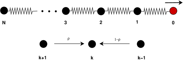
We take up the study of a system very familiar from physics ([5] for example): a long string of coupled linear oscillators (called ‘agents’ or ‘cars’ from here on) with linear nearest neighbor interactions. In order to model things like traffic we change certain features of the model that is so familiar in the context of statistical physics. The most significant ones are that we do not assume that interaction is symmetric and that the oscillators are damped. Furthermore we allow the system to have non-zero mean velocity. Finally we assume that the chain is finite and we take into account boundary effects from the ends of the chain (no periodic boundary conditions). The class of systems whose study we take up in this paper is illustrated in Figure 1.1 and made precise in Equation 2.5.
The purpose here is to gain a qualitative understanding of how a perturbation in the movement of one the agents (which we call the leader) propagates throughout the flock of agents. Here is a more precise formulation. Suppose that a flock is moving coherently or “in formation”, ie: each member has the same constant velocity, and inter-agent distances are constant. Now the leader’s motion is perturbed. After a while also the agent farthest away from the leader (called the trailing car) senses the effect, and its orbit will start to deviate from the in formation orbit. What is the ratio between these two perturbations as a function of the size of the flock, while keeping all other parameters fixed ?
The immediate motivation is to study which kinds of interactions might take place in actual large flocks or might seem desirable to implement in artificial flocks (think of cars on a highway equipped with an automatic pilot). It would seem that in both types of systems the kinds of interaction preferred would be those where the growth rate just mentioned is as low as possible.
Ideally we find the growth rate of perturbations in many different models, for example where interactions are allowed to include up to 2 or 3 or 10 neighbors on either side. This seems analytically out of reach. Thus the acceleration of the -th car is determined by its observations of the -st and the -st car. What we chose to do instead is to introduce a weighted nearest neighbor interaction, that is: For we weight the information coming from the -st car with , and the other with (see Equation (2.5)).
This line of thought has many potential applications in technology. Suppose for example one wants to automatically control dense traffic on a single lane road. Each car is equipped with sensors that register the relative velocity and position of its neighbors. This information is then used to regulate the acceleration of the cars. A typical example is the ‘canonical traffic problem’ proposed in [7] and [8], where the lead car abruptly accelerates (when, for example, a traffic light turns green), and the other cars try to follow.
Our conclusions for the systems typified by Equation 2.5, can be summarized as follows. In all systems the ratio of the size of perturbation of the trailing car to the perturbation of the leader grows exponentially in the size of the flock, with one exception: when . In the last case (called the symmetric case because equal attention is paid to the cars on either side) this growth is only linear as function of . The study of the symmetric case was reported in [7, 8]. Here we continue that program by investigating the asymmetric case.
The curious fact that perturbations in the leader’s position or velocity is necessarily unbounded as the size of the flock grows is of course of paramount importance in many applications (automated traffic, biological flocks, and so on). In fact this has been commented upon by several authors already, notably [4, 2] in cases similar to our and cases. In this note we give precise estimates for how these perturbations grow as function of the number of agents, not only in those cases but also for other models (all ).
A more distant motivation to study these systems is to attain a general understanding of linear oscillators interacting according to a more general graph (called the “communication graph”, see for instance [6] for definitions). In that context similar questions arise but in a more general context. What we present here is a simple example.
Section 2 defines the model. In Section 3 the definitions of stability we use are given and briefly discussed. In it we also state the main result of this note. Sections 4 and 5 prove these results. (Some of the more calculational steps in these proofs are relegated to the Appendix.)
Notational Conventions: To avoid confusion, we finally list two important conventions here. The first is that after Section 4 we assume that both and are negative reals to insure asymptotic stability (Theorem 4.2). The second is that in order for certain expressions ( and , for ) in Theorem 5.2) to be continuous functions it is convenient to define the symbol as the root with angle in the interval (branch cut along the positive real axis).
Acknowledgements:
I am grateful for useful conversations with Folkert Tangerman.
2 The Model
We define the model and propose a notion of stability for flocks. Our strategy is to study qualitative aspects of the solution for fixed , , and , and as we let tend to infinity.
Let and be real, and . The model is given by:
| (2.1) | |||||
| (2.2) | |||||
| (2.3) | |||||
| (2.4) | |||||
| (2.5) |
The (constant) parameters determine the desired relative distances between agents and as . The feedback parameters and are independent of and time. Note that the total number of agents is in fact also a parameter in this problem. We do not carry this into the notation. The subscript will always stand for the last agent in a system with agents numbered from 0 to . Similarly we do not carry the dependence on the parameters and explicitly into the notation.
One can show that the orbits of this system such that the distances between successive cars are preserved (namely: ) form a 2-parameter family, namely and . We will call these orbits in formation orbits.
It is advantageous to write Equation (2.5) in a more compact form. Introduce the notation
The leading car is not encoded since its orbit is a priori given. The system can now be recast as a first order ODE:
| (2.6) |
The details of this are discussed in [6], here we just give the relevant definitions.
Let and are -dimensional square matrices, where is the identity and is given by
| (2.7) |
is called the reduced graph Laplacian. It describes the flow of information among the agents, with the exception of the leader (hence the word ‘reduced’). The matrices and are given by:
| (2.8) |
The orbit of the leader is assumed to be a priori given and therefore only appears in the forcing term . We will refer to this agent as an (independent) leader. Analyzing Equation (2.5) and assuming without loss of generality that , one gathers that:
| (2.9) |
To define of Equation (2.6) in terms of these quantities, we use the Kronecker product ()
| (2.10) |
The advantage of this somewhat roundabout way of defining the matrix is that in the eigenvalues of the reduced Laplacian in many cases are known. From that the eigenvalues of can then be derived. That is the program followed in the Section 4.
3 Stability of Flocks
Definition 3.1
The system given in Equation 2.6 is called ‘asymptotically stable’ if all eigenvalues of have negative real part.
Suppose for the moment that fot . Then the solution of the system tends to 0 exponentially fast (in ) if and only if the system is asymptotically stable. This corresponds to the usual notion of asymptotic stability (see for example [1], Section 23). The question when the system is asymptotically stable has a straightforward answer (see Theorem 4.2): it is if and only if and in Equation (2.5) are negative. We will therefore from now on assume that and are negative.
One can show (Proposition 5.1) that if the leader executes an oscillation of the form , then tends to as tends to infinity. The functions are called the frequency response functions.
Definition 3.2
Let . The system is called ‘harmonically stable’ if it is asymptotically stable and if . Otherwise the system is called ‘harmonically unstable’.
This kind of instability roughly says that certain long-term oscillatory perturbations in the orbit of the leader will have their amplitude magnified by a factor that is exponentially large in . In Theorem 5.5 we establish that the system is harmonically unstable if ; harmonic stability for was established in [7].
In earlier work ([8]) we studied a ‘fundamental traffic problem’ which roughly corresponds to setting the acceleration of the leader equal to the Dirac delta function, , and . This gives for which can be substituted into Equation (2.9).
Definition 3.3
Consider Equation (2.6) with forcing determined by and subject to the initial conditions and . Let . The system is called ‘impulse stable’ if it is asymptotically stable and if for 0, 1 and 2, we have . (And ‘impulse unstable’ in the other case.)
Loosely interpreted this kind of instability means that if we give the leader a ’unit-kick’, then that perturbation travels through the flock and causes , , or to grow exponentially in , before eventually dying out (due to asymptotic stability).
Impulse stability is perhaps at first sight more natural or appealing than harmonic stability because it is formulated in the time domain, whereas the latter takes place in the Fourier domain. However mathematically the criterion is much harder to check. In [8] we proved that the case is impulse stable. But the case is much more problematic and will be taken up in a separate work ([9]).
It therefore may be argued that all three kinds of stability are necessary to form large flocks. From the above remarks, it follows that of the systems investigated here only the one with satisfies all three. It is interesting that even in that case linear growth of still takes place (see [7, 8]). This seems to be the best case possible. we summarize this discussion with our main result.
Theorem 3.4
The system given by Equation (2.5) satisfies all three stability criteria if and only if and are negative and .
4 Asymptotic Stability
We derive the criterion for asymptotical stability.
In the statement of the next result we use the following equation, where and are real variables:
| (4.1) |
Recall that the matrix is defined in Equation (2.7).
Proposition 4.1
One can show (see [6, 7, 8]) that the eigenvalues of defined in Equation (2.6) are given by the solutions of
| (4.2) |
where runs through the spectrum of . So:
Theorem 4.2
The eigenvalues of are
where runs through the spectrum of . Because the are contained in the interval (see Proposition 4.1), the system is stabilized (or asymptotically stable) if and only if both and are strictly smaller than zero.
5 Harmonic Stability
In this section we calculate (Proposition 5.2) and study the properties (Theorem 5.5) of the frequency response function of the trailing car in detail. The main result of this Section is Theorem 5.5 that says that if then the system is harmonically unstable. (If the question is moot as the leader’s motion goes unperceived by the flock.)
The following constant will frequently simplify formulae:
Proposition 5.1
If and and , there is a sequence of complex numbers so that trajectory of the system is asymptotic to:
Proof: (See also [6].) Since , the non-autonomous term in Equation (2.6) can be written as , where is a constant vector. The general solution of the system is: , and tends to zero.
The complex functions (where ) are called the frequency response (of the -th agent).
Proposition 5.2
Proof: The reasoning of i) is identical to that in Lemma 3.2 of [8].
Remark: Even though are not rational functions of , one can check that in fact the in fact are proper rational.
Remark: The coefficients in the Theorem are the roots of the following quadratic equation:
The most important case of Theorem 5.2 is the frequency response of the trailing car, labeled , when . The previous result immediately implies:
Corollary 5.3
For the frequency response function of the last agent is given by
with and as before.
Because the inverse Fourier Transform of equals the real valued function , we are mainly interested in the case where and is a positive real number (the frequency). Note that then also must equal the complex conjugate of . In fact, using Lemma 6.1 in the previous Proposition yields that . Thus it is sufficient to study only for .
Proposition 5.4
Suppose , , and are all fixed. Then, for as in Lemma 6.3, as large tends to infinity:
Proof: Use Proposition 5.2 and the fact that to rewrite
| (5.1) |
Since
it suffices to prove that if , then . Now suppose that , then the second remark after Proposition 5.2 implies that and so Lemma 6.2 implies that .
Remark: It is important to realize that the even for large but fixed , the last factor could become large if we let approximate 1. The results in the appendix can be used to show that this can happen if and only if and very close to zero. We make use of this fact in the proof (for ) of the next and main result of this section.
Theorem 5.5
For all , grows exponentially in . When , growth is linear in .
Proof: The second statement has been proved in [8]. Fix and let as in Equation 6.1. Lemma 6.4 and the remark thereafter now imply that if and only if . The result follows directly from the first part of Proposition 5.4. Finally fix , or . First use Lemma 6.1 to see that if , then and . Substitute this into the denominator of in Corollary 5.3. The leading order cancels. The next term is of order at least . Thus is of order at least .
6 Appendix: Technical Results
For completeness we collect a number of straightforward results that are necessary for development of the theory, but would clutter the exposition in the main text. Various relevant quantities are evaluated for where is real and non-negative. As observed in the main text, we use without loss of generality. The conventions mentioned in the Introduction also hold.
Lemma 6.1
i): For and small:
ii): For and small:
Proof: By sheer calculation. (See [7] for some of the computational details.)
Remark: This expansion diverges for ; in that case we have ([7]):
Lemma 6.2
.
Lemma 6.3
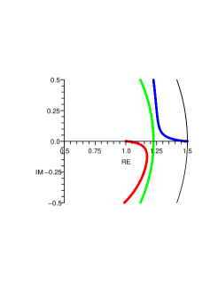
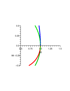
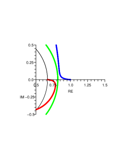
For each , the number exists and is contained in . (See Figure 6.1.)
Proof: From Lemma 6.2, when is large. Substitute this into the expression for in Theorem 5.2 to see that for large , in fact becomes very small. When , Lemma 6.1 implies that .
It is now sufficient to prove that for the absolute values are never equal. So suppose there are and so that . The first item in Theorem 5.2 gives:
Dividing this by , squaring the equation, and noting that , we see that
This implies that is a positive real and therefore is real for some , which is impossible by Lemma 6.2.
Lemma 6.4
For each , there is a unique such that
Proof: We know that and (from the proof of the previous Lemma) for large : is small. It is sufficient to prove that is the unique solution in of and that it is simple.
Consider the characteristic equation and suppose that there is a root . Then . Equate this to the expression given in Lemma 6.2 and use the fact that to obtain:
This equation factors as follows:
The second factor gives exactly one simple positive root for , yielding a unique simple positive root .
Remark: In fact,
| (6.1) |
References
- [1] V. I. Arnold, Ordinary Differential Equations, 3rd Ed, Springer, 1992.
- [2] P. Barooah, J. Hespanha, Error Amplification and Disturbance Propagation in Vehicle Strings with Decentralized Linear Control, Proc 44th Conf. on Decision and Contr., 2005.
- [3] C. M. da Fonseca, J. J. P. Veerman, On the Spectra of Certain Directed Paths, Applied Mathematics Letters 22 (2009) 1351-1355.
- [4] P. Seiler, A. Pant, K. Hedrick, Disturbance propagation in vehicle strings, IEEE Trans. Automatic Control Vol 49, Issue 10, 1835 - 1842, 2004.
- [5] F. Seitz, Modern Theory of Solids, McGraw-Hill, 1940.
- [6] J. J. P. Veerman, John S. Caughman, G. Lafferriere, A. Williams, Flocks and Formations, J. Stat.Phys. 121, Vol 5-6, 901-936, 2005.
- [7] J. J. P. Veerman, B. D. Stosic, A. Olvera, Spatial Instabilities and Size Limitations of Flocks, Networks and Heterogeneous Media, Volume 2, Number 4, December 2007.
- [8] J. J. P. Veerman, B. D. Stosic, F. M. Tangerman, Automated Traffic and The Finite Size Resonance, submitted.
- [9] J. J. P. Veerman, F. M. Tangerman, Impulse Stability of Large Flocks: an Example, in preparation.