$1/f^{\beta}$ noise in a model for weak ergodicity breaking

Abstract

In systems with weak ergodicity breaking, the equivalence of time averages and ensemble averages is known to be broken. We study here the computation of the power spectrum from realizations of a specific process exhibiting $1/f^{\beta}$ noise, the Rebenshtok–Barkai model. We show that even the binned power spectrum does not converge in the limit of infinite time, but that instead the resulting value is a random variable stemming from a distribution with finite variance. However, due to the strong correlations in neighboring frequency bins of the spectrum, the exponent $\beta$ can be safely estimated by time averages of this type. Analytical calculations are illustrated by numerical simulations.

1 Introduction

In recent years, the study of long range correlations in experimental data has moved into the focus of interest. Whereas a large amount of empirical results has been obtained using detrended fluctuation analysis [1], the same information is, in principle, also contained in the power spectrum. Observations of nontrivial power law decays of the power spectrum have a long tradition and are usually denoted by $1/f$-noise, or, more precisely, $1/f^{\beta}$ with $\beta\approx 1$. Examples include noise in electric resistors, in semiconductor devices (flicker noise), and fluctuations in geophysical data [2, 3, 4].

By weak ergodicity breaking one describes the behavior of a system which is ergodic in the sense that a single trajectory is able to explore completely some invariant component of the phase-space (it is indecomposable), but where the invariant measure is not normalizable, so that the time scales for this exploration might diverge (in other words, there is no finite microscopic time scale). This concept goes back to Bouchaud [5]. A consequence of this is that time averages computed on a single (infinite) trajectory will not converge to the ensemble mean. Instead, the time average is a random variable itself, as a function of the initial condition of the trajectory, which is drawn from a distribution with non-zero variance. It has been shown that Continuous-Time Random Walks [6], but also specific deterministic dynamical systems [7] exhibit this behavior. A natural consequence of it is the non-existence of a finite correlation time, reflected by a power law decay of the auto-correlation function, which translates itself into a $1/f^{\beta}$-behavior of the power spectrum. This type of spectrum has been derived for a two state process of this type by Margolin and Barkai [8, Eq. (33)].

As said, the crucial aspect of systems with weak ergodicity breaking is that a time average in the limit of an infinite trajectory does not converge to a sharp value but is a random variable with a distribution of finite width. This should also hold for the power spectrum. Therefore, it is not evident that an estimation of $\beta$ from a numerically computed power spectrum of a single trajectory is reliable. We therefore investigate the estimation of the power spectrum from single realizations of a specific process with weak ergodicity breaking.

A relevant remark is necessary: If one estimates the power spectrum by a discrete Fourier transform from a time series with sampling interval $\Delta t$ (i.e., uses the periodogram), then the variance of the estimator $f_{k}$ for the power contained in the $k$th discrete frequency is $f_{k}^{2}$. However, if the correlations in the time domain decay exponentially fast, then the errors in adjacent frequencies $f_{k}$ and $f_{k\pm 1}$ are sufficiently weakly correlated such that the error of a binned spectrum where one takes averages over $M$ adjacent frequencies decays like $1/\sqrt{M}$ [9, Sect.13.4]. In the limit of an infinite time series, the estimation error of the binned power spectrum of an ergodic process therefore decays to zero, i.e., the spectrum assumes uniquely defined values. In the following, we will discuss results for binned power spectra of processes with weak ergodicity breaking. The binning implies that in the analytical calculations we are allowed to ignore the time discretization which is present in every numerical data analysis.

The next Sections are devoted to an analytical derivation of the fact that the binned power spectrum of a weakly non-ergodic process is a random variable whose distribution has a non-zero variance. In addition, we compute the correlations between different bins. We will show that because of these correlations, further binning cannot reduce the uncertainty about the true power, and moreover, that the whole uncertainty about the power spectrum reduces to a random normalization factor. This has the important consequence that the power law exponent $\beta$ can indeed be estimated numerically regardless of the difficulties to estimate the spectrum itself.

In Section 5 we illustrate the analytical (asymptotic) results by numerical simulations, also opposing time averages to ensemble averages. Note that because of the long range correlations, cutting a long trajectory into pieces and treat these as an ensemble is not valid, since this ensemble would not represent an independent sample of initial conditions.

2 The model and basic approach

Rebenshtok and Barkai introduced the following model for a thermodynamic system showing weak ergodicity breaking [10, 11]: In its simplest form it is characterized by two distributions, one waiting time distribution with density $\phi(t)$ and one distribution of an observable $x\in\mathbb{R}$ according to the probability density $\kappa(x)$. In the model let $\chi_{0},\chi_{1},\dotsc$ be i.i.d. random variables distributed according to $\kappa(x)$ and let $\tau_{0},\tau_{1},\dotsc$ be i.i.d. waiting times distributed according to $\phi(t)$. The process $X(t)$ takes the value $\chi_{0}$ in the time $0\leq t<\tau_{0}$ and $\chi_{1}$ for the next time interval of length $\tau_{1}$. In general

$$X(t)=\chi_{i}\quad\text{ for }T_{i-1}\leq t<T_{i}$$ (1)

with

$$T_{i}=\sum_{j=0}^{i-1}\tau_{j}.$$ (2)

We assume that the first four moments of $\kappa(x)$ are finite, i.e.,

$$\mu_{i}=\int\textrm{d}x\,x^{i}\kappa(x)<\infty\quad\text{for }i=1,2,3,4.$$ (3)

Moreover, we assume that the distribution is centered, i.e., $\mu_{1}=0$. The waiting time distribution $\phi(t)$ should be in the domain of normal attraction of an one-sided Lévy stable distribution with exponent $\alpha$ ($0<\alpha<1$). Therefore, the Laplace transform $\hat{\phi}(\lambda)$ of $\phi(t)$,

$$\hat{\phi}(\lambda)=\int\textrm{d}t\,e^{-\lambda t}\phi(t),$$ (4)

can be expanded as

$$\hat{\phi}(\lambda)=1-(\nu\lambda)^{\alpha}+o(\lambda^{\alpha})\quad\text{as }\lambda\to 0+$$ (5)

with the scaling parameter $\nu>0$.

The Fourier transform of the time series $X(t)$ up to time $T$ is given by

$$F_{T}(\omega)=\int_{0}^{T}\textrm{d}t\,e^{i\omega t}X(t).$$ (6)

The spectrum may be estimated from

$$S_{T}(\omega)=\frac{1}{n(T)}F_{T}(\omega)F_{T}(-\omega).$$ (7)

The function $n(T)$ denotes a normalization. Normally, it takes the form $n(T)=T$, but this model requires to take $n(T)=T^{\alpha}$ for a non trivial spectrum. For finite time series one would have to add correction terms for the fact that the basis for Eq. (7) is a biased estimate of the correlation function (e.g., see [12, chapter 8.1]). These terms vanish for the asymptotic case $T\to\infty$ which we are considering here. If we have an ensemble of realizations, one can look at the unbinned spectrum

$$S_{\text{ub}}(\omega)=\lim_{T\to\infty}S_{T}(\omega).$$ (8)

Denoting the ensemble average by $\langle\cdot\rangle$, we are interested in the expectation value of the spectrum

$$\langle S_{\text{ub}}(\omega)\rangle=\lim_{T\to\infty}\frac{1}{T^{\alpha}}\langle F_{T}(\omega)F_{T}(-\omega)\rangle$$ (9)

and the covariances

$$\begin{split}\langle&S_{\text{ub}}(\omega_{1})S_{\text{ub}}(\omega_{2})\rangle\\ &=\lim_{T\to\infty}\frac{1}{T^{2\alpha}}\langle F_{T}(\omega_{1})F_{T}(-\omega_{1})F_{T}(\omega_{2})F_{T}(-\omega_{2})\rangle.\end{split}$$ (10)

The limits Eqs. (9) and (10) can be rewritten to

$$\begin{split}\langle&S_{\text{ub}}(\omega)\rangle=\biggl{.}\lim_{r\to\infty}\frac{1}{r^{\alpha}}\langle F_{rT_{1}}(\omega)F_{rT_{2}}(-\omega)\rangle\biggr{|}_{T_{1}=T_{2}=1},\\ \langle&S_{\text{ub}}(\omega_{1})S_{\text{ub}}(\omega_{2})\rangle\\ &=\biggl{.}\lim_{r\to\infty}\frac{1}{r^{2\alpha}}\begin{aligned} \langle&F_{rT_{1}}(\omega_{1})F_{rT_{2}}(-\omega_{1})F_{rT_{3}}(\omega_{2})F_{rT_{4}}(-\omega_{2})\rangle\biggr{|}_{\begin{subarray}{c}T_{1}=T_{2}=1\\ T_{3}=T_{4}=1\end{subarray}}.\end{aligned}\end{split}$$ (11)

In the following, it is helpful to define the two- and four point correlations

$$\begin{split}&C_{2}(t_{1},t_{2})=\langle X(t_{1})X(t_{2})\rangle,\\ &C_{4}(t_{1},t_{2},t_{3},t_{4})=\langle X(t_{1})X(t_{2})X(t_{3})X(t_{4})\rangle\end{split}$$ (12)

and their (double resp. quadruple) Laplace transforms

$$\begin{split}\hat{C}_{2}(\lambda_{1},\lambda_{2})&=\mathcal{L}\left[C_{2}(t_{1},t_{2})\right]\\ &=\int\textrm{d}t_{1}\,\int\textrm{d}t_{2}\,e^{-\lambda_{1}t_{1}-\lambda_{2}t_{2}}C_{2}(t_{1},t_{2}),\end{split}$$ (13)

$$\begin{split}\hat{C}_{4}(\lambda_{1},\lambda_{2},\lambda_{3},\lambda_{4})&=\mathcal{L}\left[C_{4}(t_{1},t_{2},t_{3},t_{4})\right]\\ &=\int\textrm{d}^{4}t\,e^{-\boldsymbol{\lambda}\mathbf{t}}C_{4}(\mathbf{t}).\end{split}$$ (14)

The double resp. quadruple Laplace transforms of the expressions in Eq. (11) are

$$\begin{split}\mathcal{L}&\bigl{[}\langle F_{T_{1}}(\omega)F_{T_{2}}(-\omega)\rangle\bigr{]}=\frac{1}{\lambda_{1}\lambda_{2}}\hat{C}_{2}(\lambda_{1}-i\omega,\lambda_{2}+i\omega),\\ \mathcal{L}&\bigl{[}\langle F_{T_{1}}(\omega_{1})F_{T_{2}}(-\omega_{1})F_{T_{3}}(\omega_{2})F_{T_{4}}(-\omega_{2})\rangle\bigr{]}\\ &=\frac{1}{\lambda_{1}\lambda_{2}\lambda_{3}\lambda_{4}}\hat{C}_{4}(\lambda_{1}-i\omega_{1},\lambda_{2}+i\omega_{1},\lambda_{3}-i\omega_{2},\lambda_{4}+i\omega_{2}).\end{split}$$ (15)

The limits in Eq. (11) can also be expressed in Laplace space using a formulation following the multidimensional Tauberian theorem by Drozhzhinov and Zav’jalov [13, 14] as

$$\begin{split}\mathcal{L}&\Bigl{[}\lim_{r\to\infty}\frac{1}{r^{\alpha}}\langle F_{rT_{1}}(\omega)F_{rT_{2}}(-\omega)\rangle\Bigr{]}\\ &=\lim_{\zeta\to 0+}\frac{\zeta^{\alpha}}{\lambda_{1}\lambda_{2}}\hat{C}_{2}(\zeta\lambda_{1}-i\omega,\zeta\lambda_{2}+i\omega),\end{split}$$ (16)

$$\begin{split}\mathcal{L}&\Bigl{[}\lim_{r\to\infty}\frac{1}{r^{2\alpha}}\langle F_{rT_{1}}(\omega_{1})F_{rT_{2}}(-\omega_{1})F_{rT_{3}}(\omega_{2})F_{rT_{4}}(-\omega_{2})\rangle\Bigr{]}\\ &=\lim_{\zeta\to 0+}\frac{\zeta^{2\alpha}}{\lambda_{1}\lambda_{2}\lambda_{3}\lambda_{4}}\hat{C}_{4}(\begin{aligned} \zeta&\lambda_{1}-i\omega_{1},\zeta\lambda_{2}+i\omega_{1},\\ &\zeta\lambda_{3}-i\omega_{2},\zeta\lambda_{4}+i\omega_{2}).\end{aligned}\end{split}$$ (17)

In the next section, we will show how one can calculate the Laplace transforms $\hat{C}_{n}(\boldsymbol{\lambda})$ of the multi point correlations $C_{n}(\mathbf{t})$.

However, when only one time series is given, taking $S_{T}(\omega)$ from Eq. (7) as estimate of the spectrum will lead to unsatisfactory results as the value of $S_{T}(\omega)$ will fluctuate except for some pathological cases. One often relies to the concept of binning. Instead of considering a single frequency $\omega$, one averages all available frequencies in an given interval $[\omega-\frac{1}{2}\Delta\omega,\omega+\frac{1}{2}\Delta\omega]$. For a time series of length $T$ the Fourier transform returns values at frequencies which are evenly spaced with distance $\frac{2\pi}{T}$. For large $T$ the sum can be approximated by an integral and we can consider as observable for the binned spectrum

$$S_{T}(\omega,\Delta\omega)=\frac{1}{\Delta\omega}\int_{\omega-\frac{1}{2}\Delta\omega}^{\omega+\frac{1}{2}\Delta\omega}\textrm{d}\omega^{\prime}\,S_{T}(\omega^{\prime}).$$ (18)

The spectrum can be estimated from

$$S_{\text{bin}}(\omega,\Delta\omega)=\lim_{T\to\infty}S_{T}(\omega,\Delta\omega).$$ (19)

Analytically, it is helpful to let the bin size go to zero as a last step

$$S_{\text{bin}}(\omega)=\lim_{\Delta\omega\to 0}S(\omega,\Delta\omega).$$ (20)

It is important to take the last limit at the very end. In most of the important cases, the value of $S_{\text{bin}}(\omega)$ will converge almost surely to the value of the spectrum.

In this paper, we want to consider the situation where the stochastic process $X(t)$ is the model by Rebenshtok and Barkai. The estimation of the spectrum is connected with averaging over the time series, therefore the question arises how the weak ergodicity breaking affects the observable $S_{\text{bin}}(\omega)$. Does the value of $S_{\text{bin}}(\omega)$ converge to a single value or does it converge to a non trivial probability distribution? It will turn out that the latter is the case. Unlike the observable discussed by Rebenshtok and Barkai [10, 11], it seems not to be possible to determine directly the probability distribution of $S_{\text{bin}}(\omega)$. But one can obtain important information from the moments $\langle S_{\text{bin}}(\omega)\rangle$ and $\langle S_{\text{bin}}(\omega_{1})S_{\text{bin}}(\omega_{2})\rangle$.

The first step is to look at $\langle S(\omega,\Delta\omega)\rangle$ with $2|\omega|>\Delta\omega$:

$$\langle S_{\text{bin}}(\omega,\Delta\omega)\rangle=\lim_{T\to\infty}\frac{T^{-\alpha}}{\Delta\omega}\int_{\omega-\frac{1}{2}\Delta\omega}^{\omega+\frac{1}{2}\Delta\omega}\textrm{d}\omega^{\prime}\,\langle F_{T}(\omega^{\prime})F_{T}(-\omega^{\prime})\rangle.$$ (21)

We proceed similarly to the unbinned case and formulate the limit in Laplace space (note that the Laplace transform and the $\omega$-integral commute by Fubini’s theorem and the estimate $|\langle F_{T_{1}}(\omega)F_{T_{2}}(-\omega)\rangle|\leq\mu_{2}T_{1}T_{2}$ where $\mu_{2}$ is defined in Eq. (3))

$$\begin{split}\mathcal{L}&\left[\lim_{r\to\infty}r^{-\alpha}\frac{1}{\Delta\omega}\int_{\omega-\frac{1}{2}\Delta\omega}^{\omega+\frac{1}{2}\Delta\omega}\textrm{d}\omega^{\prime}\,\langle F_{rT_{1}}(\omega^{\prime})F_{rT_{2}}(-\omega^{\prime})\rangle\right]\\ &\!=\lim_{\zeta\to 0+}\frac{\zeta^{\alpha}}{\Delta\omega}\int_{\omega-\frac{1}{2}\Delta\omega}^{\omega+\frac{1}{2}\Delta\omega}\textrm{d}\omega^{\prime}\,\frac{1}{\lambda_{1}\lambda_{2}}\hat{C}_{2}(\zeta\lambda_{1}-i\omega^{\prime},\zeta\lambda_{2}+i\omega^{\prime}).\end{split}$$ (22)

Similarly, $\langle S(\omega_{1},\Delta\omega_{1})S(\omega_{2},\Delta\omega_{2})\rangle$ with $2|\omega_{1}|>\Delta\omega_{1}$ and $2|\omega_{2}|>\Delta\omega_{2}$ can be obtained from

$$\begin{split}\langle&S_{\text{bin}}(\omega_{1},\Delta\omega_{1})S_{\text{bin}}(\omega_{2},\Delta\omega_{2})\rangle\\ &=\begin{aligned} \biggl{.}\lim_{r\to\infty}&r^{-2\alpha}\frac{1}{\Delta\omega_{1}\Delta\omega_{2}}\int_{\omega_{1}-\frac{1}{2}\Delta\omega_{1}}^{\omega_{1}+\frac{1}{2}\Delta\omega_{1}}\textrm{d}\omega_{1}^{\prime}\,\int_{\omega_{2}-\frac{1}{2}\Delta\omega_{2}}^{\omega_{2}+\frac{1}{2}\Delta\omega_{2}}\textrm{d}\omega_{2}^{\prime}\\ &\langle F_{rT_{1}}(\omega_{1}^{\prime})F_{rT_{2}}(-\omega_{1}^{\prime})F_{rT_{3}}(\omega_{2}^{\prime})F_{rT_{4}}(-\omega_{2}^{\prime})\rangle\biggl{|}_{\begin{subarray}{c}T_{1}=T_{2}=1\\ T_{3}=T_{4}=1\end{subarray}}.\end{aligned}\end{split}$$ (23)

One gets

$$\begin{split}\mathcal{L}&\biggl{[}\begin{aligned} \lim_{r\to\infty}\frac{r^{-2\alpha}}{\Delta\omega_{1}\Delta\omega_{2}}&\int_{\omega_{1}-\frac{1}{2}\Delta\omega_{1}}^{\omega_{1}+\frac{1}{2}\Delta\omega_{1}}\textrm{d}\omega_{1}^{\prime}\,\int_{\omega_{2}-\frac{1}{2}\Delta\omega_{2}}^{\omega_{2}+\frac{1}{2}\Delta\omega_{2}}\textrm{d}\omega_{2}^{\prime}\\ &\langle F_{rT_{1}}(\omega_{1}^{\prime})F_{rT_{2}}(-\omega_{1}^{\prime})F_{rT_{3}}(\omega_{2}^{\prime})F_{rT_{4}}(-\omega_{2}^{\prime})\rangle\biggr{]}\end{aligned}\\ &=\begin{aligned} \lim_{\zeta\to 0+}&\frac{\zeta^{2\alpha}}{\Delta\omega_{1}\Delta\omega_{2}}\int_{\omega_{1}-\frac{1}{2}\Delta\omega_{1}}^{\omega_{1}+\frac{1}{2}\Delta\omega_{1}}\textrm{d}\omega_{1}^{\prime}\,\int_{\omega_{2}-\frac{1}{2}\Delta\omega_{2}}^{\omega_{2}+\frac{1}{2}\Delta\omega_{2}}\textrm{d}\omega_{2}^{\prime}\frac{1}{\lambda_{1}\lambda_{2}\lambda_{3}\lambda_{4}}\\ &\hat{C}_{4}(\zeta\lambda_{1}-i\omega_{1}^{\prime},\zeta\lambda_{2}+i\omega_{1}^{\prime},\zeta\lambda_{3}-i\omega_{2}^{\prime},\zeta\lambda_{4}+i\omega_{2}^{\prime}).\end{aligned}\end{split}$$ (24)

Therefore the problem can be reduced to the determination of the Laplace transforms $\hat{C}_{n}(\boldsymbol{\lambda})$ of the $n$ point correlations functions. We describe in the next section how to obtain them.

3 A diagrammatic approach to the multi point correlation functions

In [15] a diagrammatic method was introduced how to determine the joint probability distributions and multi point correlation functions of a continuous-time random walk. In this section we are adapting this method to determine $\hat{C}_{n}(\boldsymbol{\lambda})$. For any set of natural numbers $q_{1},\dotsc,q_{n}\in\mathbb{N}_{0}$, one defines

$$C_{n}[\mathbf{q}](\mathbf{t})=\left\langle\prod_{k=1}^{n}\chi_{q_{k}}1_{[T_{q_{k}},T_{q_{k}+1}[}(t_{k})\right\rangle$$ (25)

with the indicator function ($A$ being any subset $A\subseteq\mathbb{R}$)

$$1_{A}(t)=\begin{cases}1&\text{for }t\in A,\\ 0&\text{for }t\notin A.\end{cases}$$ (26)

The $C_{n}[\mathbf{q}](\mathbf{t})$ can be considered as partial correlations which only contribute, when the time $t_{i}$ is in the $(q_{i}+1)$th waiting time (for $i=1,\dotsc,n$). Therefore,

$$\begin{split}C_{n}(\mathbf{t})&=\langle X(t_{1})\dotsm X(t_{n})\rangle\\ &=\sum_{q_{1},\dotsc,q_{n}=0}^{\infty}C_{n}[\mathbf{q}](\mathbf{t}).\end{split}$$ (27)

Define the contribution of one step as

$$\eta^{(j)}_{n}[\mathbf{q}](\mathbf{t})=\prod_{i:q_{i}=j}\chi_{j}1_{[0,\tau_{j}[}(t_{i})\prod_{i:q_{i}>j}\delta(t_{i}-\tau_{j})\prod_{i:q_{i}<j}\delta(t_{i}).$$ (28)

One obtains by induction

$$C_{n}[\mathbf{q}](\mathbf{t})=\left\langle\underset{j}{\bigstar}\eta^{(j)}_{n}[\mathbf{q}](\mathbf{t})\right\rangle$$ (29)

where $\star$ denotes the convolution in the time variable $t_{1},\dotsc,t_{n}$ and $j$ runs from $0$ to any natural number larger than $\max(q_{1},\dotsc,q_{n})$.

Transforming into Laplace space gives

$$\begin{split}\hat{C}_{n}[\mathbf{q}](\boldsymbol{\lambda})&=\mathcal{L}\left[C_{n}[\mathbf{q}](\mathbf{t})\right]\\ &=\prod_{j}\langle\hat{\eta}^{(j)}_{n}[\mathbf{q}](\boldsymbol{\lambda})\rangle.\end{split}$$ (30)

Using the following notations from [15] (suppressing the dependence on $\mathbf{q}$)

$$\mathbb{V}_{j}=\{i:q_{j}=i\},\quad\mathbb{E}_{j}=\{i:q_{i}<j\},\quad\mathbb{L}_{j}=\{i:q_{i}>j\}.$$ (31)

The set $\mathbb{V}_{j}$ (“vertex”) contains the indices which are at position $j$, the set $\mathbb{E}_{j}$ (“earlier”) contains the indices which are before that position and the set $\mathbb{L}_{j}$ (“later”) contains the indices which are after that position. With the notation

$$\Lambda_{J}=\sum_{j\in J}\lambda_{j}$$ (32)

one gets

$$\begin{split}\langle\hat{\eta}^{(j)}_{n}[\mathbf{q}](\boldsymbol{\lambda})\rangle&=\biggl{\langle}\int\mathrm{d}^{n}t\,e^{-\boldsymbol{\lambda}\mathbf{t}}\prod_{i\in\mathbb{V}_{j}}\chi_{j}1_{[0,\tau_{j}[}(t_{i})\prod_{i\in\mathbb{E}_{j}}\delta(t_{i}-\tau_{j})\prod_{i\in\mathbb{L}_{j}}\delta(t_{i})\biggr{\rangle}\\ &=\frac{\mu_{|\mathbb{V}_{j}|}}{\prod_{v\in\mathbb{V}_{j}}\lambda_{v}}\sum_{J\in P(\mathbb{V}_{j})}(-1)^{|J|}\hat{\phi}(\Lambda_{J\cup\mathbb{L}_{j}}).\\ \end{split}$$ (33)

Here, the power set of $\mathbb{V}_{j}$ is denoted by $P(\mathbb{V}_{j})$ and $|J|$ is the number of elements of $J$. Therefore, the last sum goes over all subsets $J$ of indices of $\mathbb{V}_{j}$.

Figure 1: A generic diagram

As in [15] we introduce diagrams which denote the relative ordering of the $q_{i}$s. A generic diagram is given in Fig. 1. The main idea behind this consists in grouping all steps $i$ with the same $\mathbb{V}_{i}$, $\mathbb{E}_{i}$ and $\mathbb{L}_{i}$. If $\mathbb{V}_{i}=\{\}$ then there can be several successive steps with the same $\mathbb{E}_{i}$ and $\mathbb{L}_{i}$. These successive steps are combined to a horizontal line. If $\mathbb{V}_{i}\neq\{\}$ then there can be only one step with these sets of indices. This is represented by a vertex with the indices $\mathbb{V}_{i}$ leaving. Therefore the diagram Fig. 1 represents all $\mathbf{q}$ with the following properties: First there is any number of steps $i$ with $\mathbb{E}_{i}=\{\}$, $\mathbb{V}_{i}=\{\}$ and $\mathbb{L}_{i}=L_{0}$. A single step with $\mathbb{E}_{i}=\{\}$, $\mathbb{V}_{i}=V_{1}$ and $\mathbb{L}_{i}=L_{1}$ follows. At next is any number of steps $i$ with $\mathbb{E}_{i}=V_{1}$, $\mathbb{V}_{i}=\{\}$ and $\mathbb{L}_{i}=L_{1}$. The rest in interpreted analogously. For each $n$ point correlation there is only a finite number of diagrams and summing over all $\mathbf{q}$ represented by a diagram turns out to be easy. It turns out that one can associate to each part of the diagram a factor (for a more comprehensive derivation of these results, we refer to [15]). One obtains the following rules (where $\mu_{i}$ is defined in Eq. (3))

$$\begin{split}&\gamma_{\text{vertex }i}=\frac{\mu_{|V_{i}|}}{\prod_{v\in V_{i}\lambda_{v}}}\sum_{J\in P(V_{i})}(-1)^{|J|}\hat{\phi}(\Lambda_{J\cup L_{i}}),\\ &\gamma_{\text{line }i}=\sum_{j=0}^{\infty}\hat{\phi}^{j}(\Lambda_{L_{i}})=\frac{1}{1-\hat{\phi}(\Lambda_{L_{i}})}.\end{split}$$ (34)

Since we assumed that $\mu_{1}=0$, we do not need to consider diagrams which contain vertices with only one leaving line. Therefore a single diagram remains for $\hat{C}_{2}(\lambda_{1},\lambda_{2})$ which drawn in Fig. 2a. This gives

$$\begin{split}\hat{C}_{2}(\lambda_{1},\lambda_{2})&=\gamma_{\text{line},L=\{1,2\}}\gamma_{\text{vertex},V=\{1,2\},L=\{\}}\\ &=\frac{\mu_{2}}{\lambda_{1}\lambda_{2}}\frac{1-\hat{\phi}(\lambda_{1})-\hat{\phi}(\lambda_{2})+\hat{\phi}(\lambda_{1}+\lambda_{2})}{1-\hat{\phi}(\lambda_{1}+\lambda_{2})}.\end{split}$$ (35)

Figure 2: The types of diagrams relevant for a) the two point correlation and b) four point correlation

For the four point correlation two types of diagrams are relevant, which are drawn in Fig. 2b. The contributions are

$$\begin{split}&D_{\text{I}}(\boldsymbol{\lambda})\begin{aligned} &=\gamma_{\text{line},L=\{1,2,3,4\}}\gamma_{\text{vertex},V=\{3,4\},L=\{1,2\}}\\ &\phantom{=}\times\gamma_{\text{line},L=\{1,2\}}\gamma_{\text{vertex},V=\{1,2\},L=\{\}}\end{aligned}\\ &=\frac{\mu_{2}^{2}}{\lambda_{1}\lambda_{2}\lambda_{3}\lambda_{4}}\frac{\hat{\phi}(\Lambda_{\{1,2\}})-\hat{\phi}(\Lambda_{\{1,2,3\}})-\hat{\phi}(\Lambda_{\{1,2,4\}})+\hat{\phi}(\Lambda_{\{1,2,3,4\}})}{1-\hat{\phi}(\Lambda_{\{1,2,3,4\}})}\\ &\phantom{=}\times\frac{1-\hat{\phi}(\lambda_{1})-\hat{\phi}(\lambda_{2})+\hat{\phi}(\lambda_{1}+\lambda_{2})}{1-\hat{\phi}(\lambda_{1}+\lambda_{2})}\end{split}$$ (36)

$$\begin{split}D_{\text{II}}(\boldsymbol{\lambda})=&\gamma_{\text{line},L=\{1,2,3,4\}}\gamma_{\text{vertex},V=\{1,2,3,4\},L=\{\}}\\ =&\frac{\mu_{4}}{\lambda_{1}\lambda_{2}\lambda_{3}\lambda_{4}}\frac{\sum_{J\in P(\{1,2,3,4\})}(-1)^{|J|}\hat{\phi}(\Lambda_{J})}{1-\hat{\phi}(\Lambda_{\{1,2,3,4\}})}.\end{split}$$ (37)

The function $\hat{C}_{4}(\boldsymbol{\lambda})$ is obtained by summing over all possible combinations of indices at the vertices, i.e.,

$$\begin{split}\hat{C}_{4}(\boldsymbol{\lambda})=&D_{\text{I}}(\lambda_{1},\lambda_{2},\lambda_{3},\lambda_{4})+D_{\text{I}}(\lambda_{1},\lambda_{3},\lambda_{2},\lambda_{4})\\ &+D_{\text{I}}(\lambda_{1},\lambda_{4},\lambda_{2},\lambda_{3})+D_{\text{I}}(\lambda_{2},\lambda_{3},\lambda_{1},\lambda_{4})\\ &+D_{\text{I}}(\lambda_{2},\lambda_{4},\lambda_{1},\lambda_{3})+D_{\text{I}}(\lambda_{3},\lambda_{4},\lambda_{1},\lambda_{2})\\ &+D_{\text{II}}(\lambda_{1},\lambda_{2},\lambda_{3},\lambda_{4}).\end{split}$$ (38)

4 Evaluating the spectral observables

4.1 The unbinned observables

We can use the results of the last section to determine the spectral observables. Using the expansion Eq. (5) and the two point correlations Eq. (35) to calculate the limit Eq. (16)

$$\begin{split}&\lim_{\zeta\to 0+}\frac{\zeta^{\alpha}}{\lambda_{1}\lambda_{2}}\hat{C}_{2}(\zeta\lambda_{1}-i\omega,\zeta\lambda_{2}+i\omega)\\ &\quad=\frac{1}{\lambda_{1}\lambda_{2}(\lambda_{1}+\lambda_{2})^{\alpha}}\frac{\mu_{2}}{\nu^{\alpha}}\frac{2-\hat{\phi}(i\omega)-\hat{\phi}(-i\omega)}{\omega^{2}}\end{split}$$ (39)

The Laplace transform can be inverted by using

$$\mathcal{L}\left[\frac{\min(T_{1},T_{2})^{\alpha}}{\Gamma(1+\alpha)}\right]=\frac{1}{\lambda_{1}\lambda_{2}(\lambda_{1}+\lambda_{2})^{\alpha}}.$$ (40)

Therefore, one has

$$\langle S_{\text{ub}}(\omega)\rangle=\frac{\mu_{2}}{\nu^{\alpha}\Gamma(1+\alpha)}\frac{2-\hat{\phi}(i\omega)-\hat{\phi}(-i\omega)}{\omega^{2}}$$ (41)

with the behavior near $\omega\to 0+$

$$\langle S_{\text{ub}}(\omega)\rangle=\frac{2\mu_{2}\cos\left(\frac{\pi}{2}\alpha\right)}{\nu^{\alpha}\Gamma(1+\alpha)}\frac{1}{|\omega|^{2-\alpha}}+o\left(\frac{1}{|\omega|^{2-\alpha}}\right).$$ (42)

This last equation shows that the spectrum has a $1/f^{2-\alpha}$ form near the origin.

Following [16, Lemma XV.1.3], there exists an $\Omega\geq 0$ such that

$$\hat{\phi}(i\omega)=1\quad\Leftrightarrow\quad\omega\in\Omega\mathbb{Z}.$$ (43)

The case $\Omega\neq 0$ appears if and only if the waiting times $\tau_{i}$ can take only the values $0,\frac{2\pi}{\Omega},\frac{4\pi}{\Omega},\dotsc$. Therefore, more generally,

$$\hat{\phi}(z)=\hat{\phi}(z+i\omega)\quad\text{for }\operatorname{Re}(z)\geq 0\text{ and }\omega\in\Omega\mathbb{Z}.$$ (44)

In this paper we concentrate on the spectrum for frequencies $\omega\notin\Omega\mathbb{Z}$. The frequencies $\omega\in\Omega\mathbb{Z}$ behave differently, e.g., the behavior of $S_{\mathrm{ub}}(0)$ is completely described by the result of Rebenshtok and Barkai [10, 11]. Now, we can proceed to calculate the limit Eq. (17) by looking at the terms Eqs. (36) and (37) with the parameters given in Eq. (38). We have

$$\begin{split}&\lim_{\zeta\to 0+}\zeta^{2\alpha}\begin{aligned} \Bigl{(}&D_{\text{I}}(\zeta\lambda_{1}-i\omega_{1},\zeta\lambda_{2}+i\omega_{1},\zeta\lambda_{3}-i\omega_{2},\zeta\lambda_{4}+i\omega_{2})\\ &+D_{\text{I}}(\zeta\lambda_{3}-i\omega_{2},\zeta\lambda_{4}+i\omega_{2},\zeta\lambda_{1}-i\omega_{1},\zeta\lambda_{2}+i\omega_{1})\Bigr{)}\end{aligned}\\ &=\Gamma(1+\alpha)^{2}\frac{1}{\Lambda_{\{1,2,3,4\}}^{\alpha}}\left(\frac{1}{\Lambda_{\{1,2\}}^{\alpha}}+\frac{1}{\Lambda_{\{3,4\}}^{\alpha}}\right)\langle S_{\text{ub}}(\omega_{1})\rangle\langle S_{\text{ub}}(\omega_{2})\rangle.\end{split}$$ (45)

Using the fact $\hat{\phi}(i\omega_{1})1_{\Omega\mathbb{Z}}(\omega_{1}-\omega_{2})=\hat{\phi}(i\omega_{2})1_{\Omega\mathbb{Z}}(\omega_{1}-\omega_{2})$, yields similarly

$$\begin{split}&\lim_{\zeta\to 0+}\zeta^{2\alpha}\begin{aligned} \Bigl{(}&D_{\text{I}}(\zeta\lambda_{1}-i\omega_{1},\zeta\lambda_{4}+i\omega_{2},\zeta\lambda_{2}+i\omega_{1},\zeta\lambda_{3}-i\omega_{2})\\ &+D_{\text{I}}(\zeta\lambda_{2}+i\omega_{1},\zeta\lambda_{3}-i\omega_{2},\zeta\lambda_{1}-i\omega_{1},\zeta\lambda_{4}+i\omega_{2})\Bigr{)}\end{aligned}\\ &=\Gamma(1+\alpha)^{2}\frac{1}{\Lambda_{\{1,2,3,4\}}^{\alpha}}\left(\frac{1}{\Lambda_{\{2,3\}}^{\alpha}}+\frac{1}{\Lambda_{\{1,4\}}^{\alpha}}\right)\langle S_{\text{ub}}(\omega_{1})\rangle\langle S_{\text{ub}}(\omega_{2})\rangle\\ &\phantom{=}\times 1_{\Omega\mathbb{Z}}(\omega_{1}-\omega_{2})\end{split}$$ (46)

and

$$\begin{split}&\lim_{\zeta\to 0+}\zeta^{2\alpha}\begin{aligned} \Bigl{(}&D_{\text{I}}(\zeta\lambda_{1}-i\omega_{1},\zeta\lambda_{3}-i\omega_{2},\zeta\lambda_{2}+i\omega_{1},\zeta\lambda_{4}+i\omega_{2})\\ &+D_{\text{I}}(\zeta\lambda_{2}+i\omega_{1},\zeta\lambda_{4}+i\omega_{2},\zeta\lambda_{1}-i\omega_{1},\zeta\lambda_{3}-i\omega_{2})\Bigr{)}\end{aligned}\\ &=\Gamma(1+\alpha)^{2}\frac{1}{\Lambda_{\{1,2,3,4\}}^{\alpha}}\left(\frac{1}{\Lambda_{\{1,3\}}^{\alpha}}+\frac{1}{\Lambda_{\{2,4\}}^{\alpha}}\right)\langle S_{\text{ub}}(\omega_{1})\rangle\langle S_{\text{ub}}(\omega_{2})\rangle\\ &\phantom{=}\times 1_{\Omega\mathbb{Z}}(\omega_{1}+\omega_{2}).\end{split}$$ (47)

Finally

$$\lim_{\zeta\to 0+}\zeta^{2\alpha}D_{\text{II}}(\zeta\lambda_{1}-i\omega_{1},\zeta\lambda_{4}+i\omega_{2},\zeta\lambda_{2}+i\omega_{1},\zeta\lambda_{3}-i\omega_{2})=0.$$ (48)

In A, we derive the following Laplace transform

$$\begin{split}\mathcal{L}&\begin{aligned} \biggl{[}\min(T_{1},&T_{2},T_{3},T_{4})^{\alpha}\min(T_{1},T_{2})^{\alpha}\\ &\times F(\alpha,-\alpha;1+\alpha;\frac{\min(T_{1},T_{2},T_{3},T_{4})}{\min(T_{1},T_{2})})\biggr{]}\end{aligned}\\ &=\frac{\Gamma(1+\alpha)^{2}}{\lambda_{1}\lambda_{2}\lambda_{3}\lambda_{4}}\frac{1}{\Lambda_{\{1,2,3,4\}}^{\alpha}}\frac{1}{\Lambda_{\{1,2\}}^{\alpha}}\end{split}$$ (49)

with the hypergeometric function $F(\alpha,-\alpha;1+\alpha;x)$. As

$$F(\alpha,-\alpha;1+\alpha;1)=\frac{\Gamma(1+\alpha)^{2}}{\Gamma(1+2\alpha)}$$ (50)

we obtain for the limit Eq. (11)

$$\begin{split}\langle S_{\text{ub}}(\omega_{1})S_{\text{ub}}(\omega_{2})\rangle=&2\frac{\Gamma(1+\alpha)^{2}}{\Gamma(1+2\alpha)}\langle S_{\text{ub}}(\omega_{1})\rangle\langle S_{\text{ub}}(\omega_{2})\rangle\\ &\times\left(1+1_{\Omega\mathbb{Z}}(\omega_{1}-\omega_{2})+1_{\Omega\mathbb{Z}}(\omega_{1}+\omega_{2})\right).\end{split}$$ (51)

Eq. (51) will play an important role in determining the properties of the binned case. In particular, the last equation determines the variance of $S_{\text{ub}}(\omega)$ (for $2\omega\notin\Omega\mathbb{Z}$)

$$\operatorname{Var}[S_{\text{ub}}(\omega)]=V_{\text{ub}}(\alpha)\langle S_{\text{ub}}(\omega)\rangle^{2}$$ (52)

with the function

$$V_{\text{ub}}(\alpha)=4\frac{\Gamma(1+\alpha)^{2}}{\Gamma(1+2\alpha)}-1.$$ (53)

As already mentioned in the introduction, even in the ergodic limit $\alpha\to 1$, the value $V_{\text{ub}}(1)=1$ is larger than zero and therefore the observable $S_{\text{ub}}(\omega)$ does fluctuate.

The correlation coefficient between $S_{\text{ub}}(\omega_{1})$ and $S_{\text{ub}}(\omega_{2})$ (for $2\omega_{1}\notin\Omega\mathbb{Z}$ and $2\omega_{2}\notin\Omega\mathbb{Z}$; here $\Omega$ denotes the periodicity of $\hat{\phi}(\lambda)$, see Eq. (43))

$$\rho[S_{\text{ub}}(\omega_{1}),S_{\text{ub}}(\omega_{2})]=\begin{cases}1&\text{for }\omega_{1}-\omega_{2}\in\Omega\mathbb{Z}\\ R(\alpha)&\text{for }\omega_{1}-\omega_{2}\notin\Omega\mathbb{Z}\end{cases}$$ (54)

with

$$R(\alpha)=\frac{2\Gamma(1+\alpha)^{2}-\Gamma(1+2\alpha)}{4\Gamma(1+\alpha)^{2}-\Gamma(1+2\alpha)}.$$ (55)

In many cases we have $\Omega=0$, i.e.,

$$\rho[S_{\text{ub}}(\omega_{1}),S_{\text{ub}}(\omega_{2})]=R(\alpha)\quad\text{for }|\omega_{1}|\neq|\omega_{2}|.$$ (56)

In the ergodic limit, we have $R(1)=0$. Therefore, the observations $S_{\text{ub}}(\omega_{1})$ and $S_{\text{ub}}(\omega_{2})$ of the spectrum at two different frequencies $\omega_{1}$ and $\omega_{2}$ are uncorrelated.

4.2 The binned observables

Here, we are going to use the results from the unbinned case to evaluate the limits Eqs. (22) and (24). The limits on the right hand sides of these equations can be commuted with the frequency integrals describing the binning. As this statement is not obvious, we are giving an argument.

First, we are considering $\langle S_{\text{bin}}(\omega,\Delta\omega)\rangle$ with $2|\omega|>\Delta\omega$. Then we have the simple estimate

$$|\hat{C}_{2}(\zeta\lambda_{1}-i\omega,\zeta\lambda_{2}+i\omega)|\leq\frac{1}{\omega^{2}}\frac{4}{1-\hat{\phi}(\zeta(\lambda_{1}+\lambda_{2}))}.$$ (57)

The commutativity follows by dominated convergence. Therefore, we get

$$\langle S_{\text{bin}}(\omega,\Delta\omega)\rangle=\frac{1}{\Delta\omega}\int_{\omega-\frac{1}{2}\Delta\omega}^{\omega+\frac{1}{2}\Delta\omega}\textrm{d}\omega^{\prime}\,\langle S_{\text{ub}}(\omega^{\prime})\rangle$$ (58)

and accordingly

$$\langle S_{\text{bin}}(\omega)\rangle=\langle S_{\text{ub}}(\omega)\rangle.$$ (59)

It is not surprising that the binned estimate yields also the correct expectation value for an ensemble of realizations.

The argument for $\langle S_{\text{bin}}(\omega_{1},\Delta\omega_{1})S_{\text{bin}}(\omega_{2},\Delta\omega_{2})\rangle$ (with $2|\omega_{1}|>\Delta\omega_{1}$ and $2|\omega_{2}|>\Delta\omega_{2}$) needs more work. First notice that we have the following inequality

$$|1-\hat{\phi}(\lambda+i\omega)|\geq 1-|\hat{\phi}(\lambda+i\omega)|\geq 1-\hat{\phi}(\lambda).$$ (60)

This gives the following estimates (replace the tilded variables by the corresponding permutations of the $\lambda_{i}$s and $\omega_{i}$s)

$$\begin{split}&\bigl{|}D_{\text{I}}(\zeta\tilde{\lambda}_{1}+i\tilde{\omega}_{1},\zeta\tilde{\lambda}_{2}+i\tilde{\omega}_{2},\zeta\tilde{\lambda}_{3}+i\tilde{\omega}_{3},\zeta\tilde{\lambda}_{4}+i\tilde{\omega}_{4})\bigr{|}\\ &\quad\leq\frac{1}{|\tilde{\omega}_{1}\tilde{\omega}_{2}\tilde{\omega}_{3}\tilde{\omega}_{4}|}\frac{4}{1-\hat{\phi}(\zeta\tilde{\Lambda}_{\{1,2,3,4\}})}\frac{4}{1-\hat{\phi}(\zeta\tilde{\Lambda}_{\{1,2\}})}\end{split}$$ (61)

and

$$\begin{split}&\bigl{|}D_{\text{II}}(\zeta\lambda_{1}-i\omega_{1},\zeta\lambda_{2}+i\omega_{1},\zeta\lambda_{3}-i\omega_{2},\zeta\lambda_{4}+i\omega_{2})\bigr{|}\\ &\quad\leq\frac{1}{\omega_{1}^{2}\omega_{2}^{2}}\frac{16}{1-\hat{\phi}(\zeta\Lambda_{\{1,2,3,4\}})}.\end{split}$$ (62)

By dominated convergence and Eq. (51), this leads to

$$\begin{split}&\langle S_{\text{bin}}(\omega_{1},\Delta\omega_{1})S_{\text{bin}}(\omega_{2},\Delta\omega_{2})\rangle\\ &=\frac{1}{\Delta\omega_{1}\Delta\omega_{2}}\int_{\omega_{1}-\frac{1}{2}\Delta\omega_{1}}^{\omega_{1}+\frac{1}{2}\Delta\omega_{1}}\textrm{d}\omega_{1}^{\prime}\,\int_{\omega_{2}-\frac{1}{2}\Delta\omega_{2}}^{\omega_{2}+\frac{1}{2}\Delta\omega_{2}}\textrm{d}\omega_{2}^{\prime}\,\langle S_{\text{ub}}(\omega_{1}^{\prime})S_{\text{ub}}(\omega_{2}^{\prime})\rangle\\ &=2\frac{\Gamma(1+\alpha)^{2}}{\Gamma(1+2\alpha)}\frac{1}{\Delta\omega_{1}\Delta\omega_{2}}\int\textrm{d}\omega_{1}^{\prime}\,\int\textrm{d}\omega_{2}^{\prime}\,\langle S_{\text{bin}}(\omega_{1}^{\prime})\rangle\langle S_{\text{bin}}(\omega_{2}^{\prime})\rangle\end{split}$$ (63)

or shorter

$$\langle S_{\text{bin}}(\omega_{1})S_{\text{bin}}(\omega_{2})\rangle=2\frac{\Gamma(1+\alpha)^{2}}{\Gamma(1+2\alpha)}\langle S_{\text{bin}}(\omega_{1})\rangle\langle S_{\text{bin}}(\omega_{2})\rangle$$ (64)

for all $\omega_{1},\omega_{2}\neq 0$. The additional factor present in Eq. (51) for the values $\omega_{1}-\omega_{2}\in\Omega\mathbb{Z}$ and $\omega_{1}+\omega_{2}\in\Omega\mathbb{Z}$ has vanished due to the binning.

The variance of $S_{\text{bin}}(\omega)$ turns out to be

$$\operatorname{Var}\left[S_{\text{bin}}(\omega)\right]=V_{\text{bin}}(\alpha)\langle S_{\text{bin}}(\omega)\rangle^{2}$$ (65)

with the function

$$V_{\text{bin}}(\alpha)=2\frac{\Gamma(1+\alpha)^{2}}{\Gamma(1+2\alpha)}-1.$$ (66)

For $0<\alpha<1$, the value of $V_{\text{bin}}(\alpha)$ is positive, i.e., the variance of $S_{\text{bin}}(\omega)$ does not vanish and the observable $S_{\text{bin}}(\omega)$ is a proper probability distribution. $V_{\text{bin}}(\alpha)$ describes the part of the fluctuation of the spectrum which is connected with the weak ergodicity breaking, i.e., the part that remains after binning. Correspondingly, for the ergodic limit $\alpha\to 1$, the function $V_{\text{bin}}(\alpha)$ vanishes ($V(1)=0$) and the observable $S_{\text{bin}}(\omega)$ does not fluctuate.

In general, the whole spectrum is estimated. The question arises, how the weak ergodicity breaking affect different frequencies. Is it possible that one would estimate a wrong exponent $\beta$ of the $1/f^{\beta}$ noise? This can be answered by using Eq. (64) to calculate the correlation coefficient for all $0<\alpha<1$ and $\omega_{1},\omega_{2}\neq 0$:

$$\rho\left[S_{\text{bin}}(\omega_{1}),S_{\text{bin}}(\omega_{2})\right]=1.$$ (67)

This implies that $S_{\text{bin}}(\omega_{1})$ and $S_{\text{bin}}(\omega_{2})$ are linearly coupled

$$S_{\text{bin}}(\omega_{2})=\frac{\langle S_{\text{bin}}(\omega_{2})\rangle}{\langle S_{\text{bin}}(\omega_{1})\rangle}S_{\text{bin}}(\omega_{1}).$$ (68)

Therefore, as soon as one value of the spectrum is evaluated, the other values follows from this one. In other words, the weak ergodicity breaking does only affect a random prefactor which is the same for all frequencies.

5 Numerical Verification

In order to verify the presented analytical results we have performed numerical realizations of the process described above. To this purpose we have generated time series according to the following procedure:

• Pick random numbers, $\tau_{i}$, from a totally asymmetric Lévy $\alpha$-stable distribution with a given $\alpha$. These numbers represent the waiting times. The random numbers were generated by means of the procedure introduced in [17] with the scaling parameter set to one.

• Pick additional random numbers, $\chi_{i}$, from a normal distribution. These numbers are the values of the process during the respective time intervals.

• The values $\chi_{i}$ are written into the entries of an array, $A_{j}$, of total length $L$, for $j\in[\Delta t\sum_{k=1}^{i-1}\tau_{k},\Delta t\sum_{k=1}^{i}\tau_{k}[$. In all simulations presented here we chose $\Delta t=0.25$, defining the minimal resolution of the process.

The unbinned spectra, $S_{\mathrm{ub}}(\omega)$, can than be determined straight forwardly by means of the fast Fourier transform of the array $\mathbf{A}$. Of course, the spectra obtained for these processes are discrete. In order to obtain the binned spectra, $S_{\mathrm{bin}}(\omega,\Delta\omega)$, we average $S_{\mathrm{ub}}$ over various consecutive frequencies and assign the obtained value to the average of these frequencies.

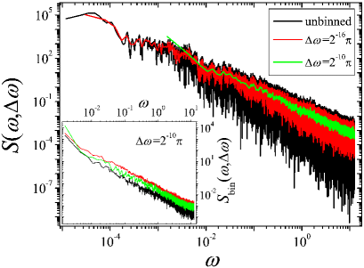
Figure 3: Power spectra corresponding to a single realization of the waiting time process are plotted for $\alpha=0.5$ for the unbinned case as well as for two different choices of the bin size. In the inset we show spectra corresponding to different realizations of the same process for a fixed choice of the binning for $\alpha=0.5$. Note that the curves exhibit a shift with respect to one another.

In Fig. 3 we plot the unbinned spectrum of a typical realization of a process of length $L=2^{21}$ for $\alpha=0.5$ together with the binned spectra for two choices of the binning, $\Delta\omega=2^{-16}\pi$, and $\Delta\omega=2^{-10}\pi$, respectively. It should be observed how the spectra get smoother when increasing the bin size, while the average slope of the spectra is not changed by the binning. Deviations from the power law behavior at small and large frequencies stem from the finite size of array $\mathbf{A}$ and the minimal resolution of the process, respectively.

The inset of Fig. 3 shows the binned spectrum with $\Delta\omega=2^{-10}\pi$ for various realizations of the processes with length $L=2^{21}$ for $\alpha=0.5$. Note that, while the exponent characterizing the decay of the spectrum does not depend on the realization, the normalization factor of the spectrum does. We would like to emphasize that the normalization factor will neither converge by increasing the length of the process nor by choosing larger bins. This probabilistic property of the normalization factor is a consequence of the weak ergodicity breaking.

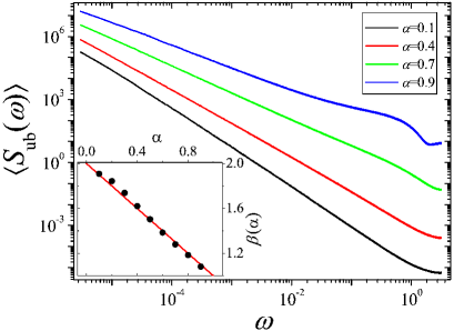
Figure 4: The averaged unbinned spectra corresponding to various choices of $\alpha$ are plotted. Note that the spectra show an algebraic decay over various decades of $\omega$ with an exponent $\beta$ depending on $\alpha$. The curves have been shifted for better visibility. In the inset we compare the theoretical prediction for the exponent $\beta$ (solid line) to the numerical findings (dots).

To verify our predictions with respect to the dependence of the spectrum on $\alpha$, we have considered the unbinned spectrum averaged over 10000 realizations of the process, $\langle S_{\mathrm{ub}}(\omega)\rangle$. In Fig. 4 we plot $\langle S_{\mathrm{ub}}(\omega)\rangle$ for processes of length $L=2^{21}$ and $\alpha=0.1,0.4,0.7,0.9$ (bottom to top), respectively. The curves have been shifted with respect to one another for better visibility. Note that the spectra show a $\sim 1/\omega^{\beta}$ behavior over various decades with an an exponent $\beta$ that decreases with increasing $\alpha$. In the inset of Fig. 4 we compare our prediction for the value of the exponent $\beta(\alpha)=2-\alpha$ (solid line), see Eq. (42), to the values obtained numerically by means of measuring the slope of the spectra in log-log scale at the intermediate region. A fairly good agreement is observed.

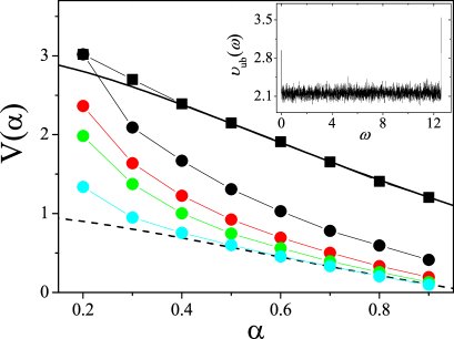
Figure 5: The theoretical predictions for $V(\alpha)$ are plotted for the unbinned (solid line) and binned (dashed line) case. Numerical results for the unbinned and the binned case are represented by the square and circular dots, respectively. In the binned case, various choices of process length have been considered, $L=2^{13},2^{15},2^{17},2^{23}$ (top to bottom). The inset shows the proportionality factor between the spectrum and the square root of the variance for the unbinned case, $\upsilon_{\mathrm{ub}}(\omega)=\mathrm{Var}[S_{\mathrm{ub}}(\omega)]/\langle S_{\mathrm{ub}}(\omega)\rangle^{2}$, for $\alpha=0.5$. Note that it is constant over various decades.

Let us now check the predictions with respect to the variance of the spectra. To calculate the variance of the unbinned spectra we have considered processes of length $L=2^{21}$ and averaging was carried out over 10000 realizations of the process. In accordance with Eq. (52) it is found that the variance is proportional to the squared expectation value of the spectrum over various decades with deviations at very high and very small frequencies only (see inset of Fig. 5). To determine the proportionality factor we have averaged this factor over the intermediate frequency region. In Fig. 5 the theoretical prediction Eq. (53) for the proportionality factor $V_{\mathrm{ub}}(\alpha)$ (solid line) is compared to the numerical results (square dots), for various choices of $\alpha$. We find a reasonable correspondence with deviations at very small $\alpha$. However, these deviations become smaller when considering longer process lengths.

To verify the predictions for the asymptotic behavior of binned spectra we have considered processes of various lengths, $L=2^{13},2^{15},2^{17},2^{23}$, while the size of the bins in frequency space was kept fixed at $\Delta\omega=2^{-8}\pi$. Note that, by augmenting the process length while keeping the bin size fixed, the number of frequencies of the discrete spectrum falling into a specific bin increases. Again, the averaging was carried out over 10000 realizations of each process. In Fig. 5 the theoretical prediction for $V_{\text{bin}}(\alpha)$ for the binned case (dashed line), see Eq. (66), is compared to the numerical data obtained for the binned processes (circular dots). It should be observed that, as the length of the process is increased (top to bottom), the values of $V_{\text{bin}}$ depart from the predictions of the unbinned case (solid line) and approach the predictions for the binned case (dashed line).

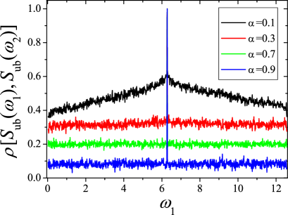
Figure 6: $\rho[S_{\mathrm{ub}}(\omega_{1}),S_{\mathrm{ub}}(\omega_{2})]$ is plotted for $\omega_{1}=2\pi$ and various choices of $\alpha$. The curves shift upwards as $\alpha$ is decreased. The peak appears at $\omega_{1}=\omega_{2}$. For very small $\alpha$ the peak extends over the whole frequency domain.

Next, we have verified our predictions with respect to the correlation coefficient of the spectra. For the unbinned case we have again considered processes of length $L=2^{21}$ and averaged over 10000 realizations. In Fig. 6, the correlation coefficient of the unbinned spectrum, $\rho[S_{\mathrm{ub}}(\omega_{1}),S_{\mathrm{ub}}(\omega_{2})]$, is plotted for the fixed frequency $\omega_{1}=2\pi$ and various choices of $\alpha$. Note that the correlation coefficient for not too small $\alpha$ is indeed flat (apart from the trivial peak at $\omega_{1}=\omega_{2}$) and that its value increases for decreasing $\alpha$. For very small values of $\alpha$ the peak around $\omega_{1}=\omega_{2}$ gets extended over the whole frequency domain but this effect can be remedied by considering longer process lengths.

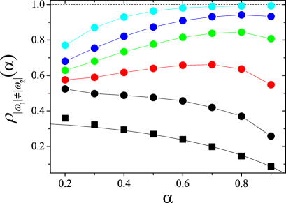
Figure 7: The theoretical predictions for $\rho_{|\omega_{1}|\neq|\omega_{2}|}(\alpha)$ are plotted for the unbinned (solid line) and binned (dashed line) case. Numerical results for the unbinned and the binned case are represented by the square and circular dots, respectively. In the binned case, various choices of process length have been considered, $L=2^{13},2^{15},2^{17},2^{19},2^{23}$ (bottom to top).

In Fig. 7 we compare the predicted value for the correlation coefficient in the unbinned case (solid line), $\rho_{|\omega_{1}|\neq|\omega_{2}|}(\alpha)=R(\alpha)$, see Eq. (55), with the numerically obtained data (squared dots). For the numerical data the correlation coefficient was averaged over $2^{16}$ choices of the pairs $\omega_{1}$ and $\omega_{2}$. Reasonable agreement between theory and numerical data is found with deviations at small $\alpha$ values stemming from the broadening of the peak around $|\omega_{1}|=|\omega_{2}|$.

Finally, we repeated the analysis of the correlation coefficient for the binned spectra. Again, we considered processes of various lengths, $L=2^{13},2^{15},2^{17},2^{19},2^{23}$, while keeping the bin size fixed in frequency space with $\Delta\omega=2^{-8}\pi$. In Fig. 7 the theoretical prediction for the correlation coefficient, $\rho_{|\omega_{1}|\neq|\omega_{2}|}(\alpha)=1$, see Eq. (67), is plotted as dotted line while the numerical data is represented by the circular dots. As the length of the process is increased, the numerical values for $\rho_{|\omega_{1}|\neq|\omega_{2}|}$ depart from the theoretical prediction for the unbinned case (solid line) and approach the predicted line for the binned case (dashed line).

6 Summary

In this paper, we have determined the spectral properties of a model by Rebenshtok and Barkai which shows weak ergodicity breaking. The analytical results were verified by numerical simulations. Near the origin, the spectrum shows a typical $1/f^{2-\alpha}$ behavior with $\alpha$ characterizes the tail behavior of the waiting time. Using a single time series will result in fluctuations of the unbinned spectrum which are also seen in the ergodic case. Therefore, one commonly uses binning to determine reliable values. While the fluctuations of the binned spectral observable vanish in the ergodic case, this is not the case for weak ergodicity breaking. However, the fluctuation does only affect a common prefactor for the whole spectrum. Consequently, the measurement of the exponent $\beta$ of the $1/f^{\beta}$ behavior is not hindered by the weak ergodicity breaking.

Recently, the emergence of universal fluctuation for processes with weak ergodicity breaking has been discussed by He et al. [18], Sokolov et al. [19] and Esposito et al. [20]. It has been shown that for several time averaged observables as the average mean square displacement the fluctuations are described by a Mittag–Leffler distribution. As can be infered from Eqs. (65) and (66), the first two moments of the binned spectrum are also in agreement with the assumption of a Mittag–Leffler distribution. However, it remains to be seen in a future work if the binned spectrum does also belong to this universality class.

The analytical results for the binned spectrum are valid in the limit of infinite time series length. In a numerical realization of this, binning means averaging only over a finite number of discrete frequencies due to the finite process time. It is therefore a nontrivial observation that these binned spectra converge for numerical manageable process lengths towards the theoretical prediction.

Appendix A Calculation of the quadruple Laplace transform

In this appendix, we derive the Laplace transform Eq. (49). We want to mention that it is possible to obtain and motivate this result by the more general methods discussed in the derivation of Eq. (71) in [15]. First consider the function

$$g(\mathbf{t})=\delta(t_{1}-t_{2})(t_{2}-t_{3})^{\alpha-1}\theta(t_{2}-t_{3})\delta(t_{3}-t_{4})t_{4}^{\alpha-1}$$ (69)

with the Dirac delta $\delta(t)$ and the Heaviside step function $\theta(t)$. Its quadruple Laplace transform can be directly calculated:

$$\mathcal{L}[g(\mathbf{t})]=\frac{\Gamma(1+\alpha)^{2}}{\alpha^{2}}\frac{1}{\Lambda_{\{1,2,3,4\}}^{\alpha}}\frac{1}{\Lambda_{\{1,2\}}^{\alpha}}.$$ (70)

Integration yields

$$\begin{split}&\int_{0}^{T_{1}}\textrm{d}t_{1}\,\int_{0}^{T_{2}}\textrm{d}t_{2}\,\int_{0}^{T_{3}}\textrm{d}t_{3}\,\int_{0}^{T_{4}}\textrm{d}t_{4}\,g(\mathbf{t})\\ &\quad=\frac{1}{\alpha}\int_{0}^{\min(T_{1},T_{2},T_{3},T_{4})}\textrm{d}t\,\left(\min(T_{1},T_{2})-t\right)^{\alpha}t^{\alpha-1}\\ &\quad=\frac{1}{\alpha^{2}}\min(T_{1},T_{2})^{\alpha}\min(T_{1},T_{2},T_{3},T_{4})^{\alpha}\\ &\qquad\times F\left(\alpha,-\alpha;1+\alpha;\frac{\min(T_{1},T_{2},T_{3},T_{4})}{\min(T_{1},T_{2})}\right).\end{split}$$ (71)

Eq. (49) follows from the properties of the Laplace transform with respect to integration.

References

References

• [1] C.-K. Peng, S. Havlin, H. E. Stanley, A. L. Goldberger, Quantification of scaling exponents and crossover phenomena in nonstationary heartbeat time series, Chaos: An Interdisciplinary Journal of Nonlinear Science 5 (1) (1995) 82–87.
• [2] M. B. Weissman, $1/f$ noise and other slow, nonexponential kinetics in condensed matter, Rev. Mod. Phys. 60 (2) (1988) 537–571.
• [3] F. N. Hooge, T. G. M. Kleinpenning, L. K. J. Vandamme, Experimental studies on 1/f noise, Reports on Progress in Physics 44 (5) (1981) 479–532.
• [4] M. Balasco, V. Lapenna, L. Telesca, $1/f^{\alpha}$ fluctuations in geoelectrical signals observed in a seismic area of southern italy, Tectonophysics 347 (4) (2002) 253 – 268.
• [5] J. P. Bouchaud, Weak ergodicity breaking and aging in disordered systems, Journal de Physique I 2 (9) (1992) 1705–1713.
• [6] G. Bel, E. Barkai, Weak ergodicity breaking in the continuous-time random walk, Physical Review Letters 94 (24) (2005) 240602.
• [7] G. Bel, E. Barkai, Weak ergodicity breaking with deterministic dynamics, Europhysics Letters 74 (1) (2006) 15–21.
• [8] G. Margolin, E. Barkai, Nonergodicity of a time series obeying Lévy statistics, Journal of Statistical Physics 122 (1) (2006) 137–167.
• [9] W. H. Press, S. A. Teukolsky, W. T. Vetterling, B. P. Flannery, Numerical recipes in FORTRAN : the art of scientific computing, 2nd Edition, Cambridge University Press, Cambridge, 1986.
• [10] A. Rebenshtok, E. Barkai, Distribution of time-averaged observables for weak ergodicity breaking, Physical Review Letters 99 (21) (2007) 210601.
• [11] A. Rebenshtok, E. Barkai, Weakly non-ergodic statistical physics, Journal of Statistical Physics 133 (3) (2008) 565–586.
• [12] K.-D. Kammeyer, K. Kroschel, Digitale Signalverarbeitungs - Filterung und Spektralanalyse mit MATLAB-Übungen, 6th Edition, Teubner, Wiesbaden, 1989.
• [13] J. N. Drozhzhinov, B. I. Zav’jalov, Tauberian theorems for generalized functions with supports in cones, Mathematics of the USSR - Sbornik 36 (1) (1980) 75–86.
• [14] Y. N. Drozhzhinov, A multidimensional Tauberian theorem for holomorphic functions of bounded argument and the quasi-asymptotics of passive systems, Mathematics of the USSR - Sbornik 45 (1) (1983) 45–61.
• [15] M. Niemann, H. Kantz, Joint probability distributions and multipoint correlations of the continuous-time random walk, Physical Review E 78 (5) (2008) 051104.
• [16] W. Feller, An Introduction to Probability Theory and Its Applications - Volume II, 2nd Edition, John Wiley & Sons, New York, 1971.
• [17] R. Weron, Levy-stable distributions revisited: tail-index $>2$ does not exclude the levy-stable regime, International Journal of Modern Physics C 12 (2) (2001) 209–223.
• [18] Y. He, S. Burov, R. Metzler, E. Barkai, Random time-scale invariant diffusion and transport coefficients, Physical Review Letters 101 (5) (2008) 058101.
• [19] I. M. Sokolov, E. Heinsalu, P. Hänggi, I. Goychuk, Universal fluctuations in subdiffusive transport, Europhysics Letters 86 (3) (2009) 30009.
• [20] M. Esposito, K. Lindenberg, I. M. Sokolov, On the relation between event-based and time-based current statistics, Europhysics Letters 89 (1) (2010) 10008.