Numerical Models of Sgr A*

Abstract

We review results from general relativistic axisymmetric magnetohydrodynamic simulations of accretion in Sgr A*. We use general relativistic radiative transfer methods and to produce a broad band (from millimeter to gamma-rays) spectrum. Using a ray tracing scheme we also model images of Sgr A* and compare the size of image to the VLBI observations at 230 GHz. We perform a parameter survey and study radiative properties of the flow models for various black hole spins, ion to electron temperature ratios, and inclinations. We scale our models to reconstruct the flux and the spectral slope around 230 GHz. The combination of Monte Carlo spectral energy distribution calculations and 230 GHz image modeling constrains the parameter space of the numerical models. Our models suggest rather high black hole spin ($a_{*}\approx 0.9$), electron temperatures close to the ion temperature ($T_{i}/T_{e}\sim 3$) and high inclination angles ($i\approx 90\hbox{${}^{\circ}$}$).

¹Department of Physics, University of Illinois, 1110 West Green Street, Urbana, IL 61801
²Astronomy Department, University of Illinois, 1002 West Green Street, Urbana, IL 61801

1. Introduction

Observations of the Galactic Center provide strong evidence for the existence of a supermassive black hole in Sgr A* (which hereafter refers to the black hole, the accretion flow, and the radio source). Sgr A*’s proximity allows us to perform observations with higher angular resolution than other galactic nuclei. Estimates of Sgr A*’s mass $M=4.5\pm 0.4\times 10^{6}M_{\odot}$ and distance $D=8.4\pm 0.4$ kpc (Ghez et al. 2008, Gillessen et al. 2009) indicate that it has the largest angular size of any known black hole ($GM/(c^{2}D)\simeq 5.3{\rm\mu as}$).

Recent 230 GHz VLBI constrains the structure of Sgr A* on angular scales comparable to the size of the black hole horizon (Doeleman et al. 2008, see also Doeleman contribution to this conference proceeding). Using a two-parameter, symmetric Gaussian brightness distribution model VLBI infers a full width at half maximum FWHM $=37^{+16}_{-10}$ ${\rm\mu as}$. This is smaller than the apparent diameter of the black hole: $\approx 2\sqrt{27}GM/(c^{2}D)\simeq 55{\rm\mu as}$ (this depends only weakly on black hole spin). Sgr A* radio - submm emission is usually modeled as synchrotron emission, with the turnover at $\sim 230$ GHz indicating transition from optically thick to optically thin emission. The model of accretion and its geometry is still under debate because Sgr A* is dim at shorter wavelengths (in NIR and X-ray band) or completely obscured (UV and optical light). Moreover in the NIR and X-ray the source is not resolved and we only have upper limits for its quiescent luminosity.

Sgr A* is a strongly sub-Eddington source ($L_{Bol}\approx 10^{-9}L_{Edd}$). Models suggest that the source is accreting inefficiently (in the sense that $L_{bol}/(\dot{M}c^{2})\ll 1$), which justifies treating the dynamics of the flow and its radiative properties independently. Therefore most of Sgr A* models published to this day consists of two separate parts: plasma dynamics model and/or radiative transfer model. We can further categorize the dynamical models into: accretion flow vs. outflow models, stationary vs. time-dependent, Newtonian/post-Newtonian vs. General Relativistic, models covering small region (a couple of gravitational radii) vs. large region (thousands of gravitational radii). The radiative transfer modeling usually uses ray tracing (always relativistic) or Monte Carlo methods (nonrelativistic as well as fully relativistic). Ray tracing allows one to model source images at sub-mm frequencies and the SED of direct synchrotron emission (radio,sub-mm). Monte Carlo allows one to model the Compton scattering and multiwavelength (from radio to gamma-rays) SED of Sgr A*. In Table 1 we summarize the recent progress in models.

Reference	dynamical	radiative	plasma	range
	model	model		of model
Narayan et al. (1998)	stat. rel. ADAF	non-rel. MC	th	$10^{5}R_{g}$
Markoff et al. (2001)	Jet	scaling	non-th	–
Yuan et al. (2003)	stat non-rel. RIAF	non-rel rays	th+non-th	$2\times 10^{5}R_{g}$
Ohsuga et al. (2005)	MHD-time dep.	non-rel. MC	th	$60R_{g}$
Goldston et al. (2005)	MHD-time dep.	polarized non-rel. rays	th+non-th	$512R_{g}$
Broderick & Loeb (2006b)	stat. non-rel RIAF	polarized RT	non-th	$2\times 10^{5}R_{g}$
Mościbrodzka et al. (2007)	MHD-time dep.	non-rel. MC	th+non-th	$2.4\times 10^{3}R_{g}$
Loeb & Waxman (2007)	Jet	scaling	th+non-th	–
Huang et al. (2007)	stat. RIAF	RT	th	$2\times 10^{5}R_{g}$
Markoff et al. (2007)	Jet	non-rel rays /w corr	non-th	–
Huang et al. (2009)	stat. rel. RIAF	RT	th	$10^{4}R_{g}$
Broderick et al. (2009)	stat. rel. RIAF	RT	th+non-th	$2\times 10^{5}R_{g}$
Chan et al. (2009)	MHD-time dep.	non-rel rays /w corr.	th+non-th	$43R_{g}$
Yuan et al. (2009)	stat. rel. RIAF	RT	th	$100R_{g}$
Hilburn et al. (2009)	GRMHD-time dep.	non-rel MC	th	$40R_{g}$
Dexter et al. (2009)	GRMHD-time dep.	RT	th	$40R_{g}$
Mościbrodzka et al. (2009)	GRMHD-time dep.	RT + rel. MC	th	$40R_{g}$

Table 1.: Summary of selected models of Sgr A*. Abbreviations: RT-ray tracing, MC-Monte Carlo, GR-general relativistic, RIAF-radiatively inefficient accretion flow, ADAF-advection dominate accretion flow, plasma-particles distribution, th-thermal, non-th-non-thermal, range-model radial range.

2. Methodology

Our numerical model of accretion onto Sgr A* consist of: a physical model of the accretion flow dynamics with its numerical realization, and a radiative transfer model. We assume that the accreting plasma is geometrically thick, optically thin, turbulent and it accretes onto a spinning black hole. The spin angular momentum $J$ of the black hole, whose magnitude is parameterized by $a_{*}=Jc/(GM^{2})$, is assumed to be aligned with the angular momentum of the accretion flow.

The accretion flow in Sgr A* is collisionless. We assume that ions and electrons have thermal distributions, possibly with different temperatures. In our model we allow the electron temperature $T_{e}$ to differ from the ion temperature $T_{i}$, but we fix the ratio ($T_{i}/T_{e}=const$). The plasma equation of state is described by the $P=e(\gamma-1)$ relation with $\gamma=13/9$ (non-relativistic ions and relativistic electrons). A more physical model would evolve $T_{e}$ and $T_{i}$ independently with a model for dissipation and energy exchange between the electrons and ions, but this would complicate the model and introduce a host of new parameters.

We realize the physical model using an axisymmetric version of the GRMHD code harm (Gammie et al. 2003). As initial conditions we adopt an analytical model of a thick disk (a torus) in hydrostatic equilibrium (Fishbone & Moncrief 1976). Since the code is not designed to evolve MHD equations in vacuum, we surround the equilibrium torus with a hot, low density plasma which does not influence the torus evolution. We seed the torus with a poloidal, concentric loops of weak magnetic field. Small perturbations are added to the internal energy which allows to for magnetorotational instability and turbulence development. We solve the GRMHD evolution equations of evolution until a quasi-equilibrium accretion flow is established (meaning that the flow is not evolving on the dynamical timescale). The details of torus initial setup and discussion of the flow evolution is presented in McKinney & Gammie (2004).

Our numerical domain extends from the black hole event horizon to $40GM/c^{2}=1.8$ AU or $210\mu as$, but is only in equilibrium to $\sim 15GM/c^{2}=0.7$AU or $80\mu as$. Since low frequency emission from Sgr A* is believed to arise at larger radius, we are unable to model the low frequency (radio, mm) portion of spectral energy distribution (SED). Our (untested) hypothesis is that at $r<15GM/c^{2}$ the model accurately represent the inner portions of a relaxed accretion flow extending over many decades in radius.

Our fluid dynamical model is scale free but the radiative transfer calculation is not. Therefore we need to specify the simulation length unit ${\mathcal{L}}=GM/c^{2}$, time unit ${\mathcal{T}}=GM/c^{3}$, and mass unit ${\mathcal{M}}$ (which scales the mass accretion rate). ${\mathcal{L}}$ and ${\mathcal{T}}$ are defined by the black hole mass adopted from observations. ${\mathcal{M}}$ is a free parameter set to reproduce the submillimeter flux $F_{230GHz}=3.4Jy$, (Marrone 2006). To “observe” the numerical model we need to specify the inclination $i$ of the black hole spin to the line of sight. The distance to the observer is assumed to be $D=8.4kpc$.

The SED is calculated in a Monte Carlo fashion. We use grmonty - a general relativistic radiative transfer scheme (Dolence et al. 2009) to calculate the light propagation in the strong gravity taking into account synchrotron emission and absorption and Compton scattering. grmonty has been extensively tested. As one of our tests we compared the code performance in a flat space with independent Monte Carlo scheme Sphere (kindly provided by its author, Shane Davies). In Fig.1 we present a standard test for Compton scattering in the spherical, homogenous, cloud of hot plasma (Pozdniakov et al. 1979).

Figure 1.: Code testing: grmonty (points) and Sphere (independent Monte Carlo code for radiative transfer, solid line) SED comparison. In this test problem a thermal point source emits photons from the center of the spherical, hot plasma cloud. The cloud is characterized by two parameters: optical thickness $\tau$ (here $\tau=0.1$) and electron temperature $\Theta_{e}$ ($\Theta_{e}=kT_{e}/m_{e}c^{2}=4.$). Lower panel shows the difference between two SEDs.

In the present models we compute spectra through a time slice of a simulation as if the light had infinite speed (’fast light’ approximation). In reality the light crossing time is comparable to the dynamical time which suggest radiative transfer through the changing medium ($t_{dyn}\sim t_{cross}\sim 20$s in Sgr A*). Finally we use a ray-tracing scheme, ibothros (Noble et al. 2007), which accounts only for synchrotron emission and absorption in order to calculate the 230 GHz intensity maps of an accretion flow as seen by a distant observer (again in the fast light approximation). To estimate the size of the emitting region we calculate the eigenvalues of the matrix formed by taking the second angular moments of the image one the sky (the lengths of the principal axes). The eigenvalues along the major and minor axis are then compared to the FWHM VLBI constraint.

We accept or reject numerical models based on several observational constraints: the flux at 230 GHz (we scale our models to reconstruct the flux F=3.4 Jy at 230 GHz), submillimeter spectral slope $\alpha$ around a turn over frequency (230-690 GHz, $\alpha$ changing from -0.46 to 0.08 Marrone 2006), upper limit for near-IR quiescent luminosity (e.g. Genzel et al. 2003), an upper limit for X-ray luminosity $L_{X}<2.4\times 10^{33}[ergs^{-1}]$ (Baganoff et al. 2003), size of the image at 230 GHz (Doeleman et al. 2008). We compare only time-averaged SEDs and time-averaged images to the observations.

3. Results

Best-bet model

We vary three (free) model parameters: spin of the black hole ($a_{*}$=0.5, 0.75, 0.84, 0.94, 0.96, 0.98), the ion to electron temperature ratio ($T_{i}/T_{e}=1,3,10$), and inclination of the observer with respect to the spin axis ($i=5^{\hbox{${}^{\circ}$}},45^{\hbox{${}^{\circ}$}}$, and $85^{\hbox{${}^{\circ}$}}$). In Table 2 we show a set of accretion flow models in which SEDs are consistent with multiwavelength data as observed at at least one inclinations. We find the “best-bet” model, that best satisfies all the observational constraints (including VLBI 230 GHz size constrains) has spin $a_{*}=0.94$, $T_{i}/T_{e}=3$ and $i=85^{\hbox{${}^{\circ}$}}$. All other models are inconsistent with the observed SED or only marginally consistent with the VLBI size measurement.

run	$a_{*}$	$i$	$<\dot{M}\cdot 10^{-9}>$	$\alpha$	$\log_{10}L_{X}$	$\eta$	cons.
		[deg]	$[M_{\odot}/yr^{-1}]$		$[ergs^{-1}]$		w/ obs.?
		5	1.9	-1.68	31.5	$3.5\times 10^{-2}$	NO
D3	0.94	45	1.7	-1.27	31.8	$3.1\times 10^{-2}$	NO
		85	1.86	-0.44	32.9	$3.4\times 10^{-2}$	YES
		5	90.8	-1.37	30.1	$5.4\times 10^{-4}$	NO
A10	0.5	45	117.1	-0.2	31.4	$6.7\times 10^{-4}$	YES
		85	369.0	1.38	33.5	$1.6\times 10^{-3}$	NO
		5	38.3	-1.05	30.0	$1.6\times 10^{-3}$	NO
B10	0.75	45	50.2	0.04	31.8	$2.0\times 10^{-3}$	YES
		85	190.6	1.49	34.6	$6.9\times 10^{-3}$	NO
		5	19.5	-1.15	31.4	$5.1\times 10^{-3}$	NO
C10	0.875	45	23.6	-0.07	32.0	$6.2\times 10^{-3}$	YES
		85	41.4	1.19	34.2	$1.7\times 10^{-2}$	NO
		5	13.7	-0.93	31.8	$1.1\times 10^{-2}$	NO
D10	0.94	45	15.2	-0.05	32.3	$1.1\times 10^{-2}$	YES
		85	31.2	1.17	34.4	$2.5\times 10^{-2}$	NO
		5	13.6	-0.40	32.5	$2.6\times 10^{-2}$	YES
E10	0.97	45	14.3	0.2	33.1	$2.8\times 10^{-2}$	NO
		85	26.5	1.19	35.2	$5.1\times 10^{-2}$	NO
		5	9.07	-0.6	32.7	$5.3\times 10^{-2}$	YES
F10	0.98	45	9.16	-0.08	33.2	$5.2\times 10^{-2}$	NO
		85	15.5	1.12	35.4	$9.0\times 10^{-2}$	NO

Table 2.: Chosen set of models with temperature ratio 3 and 10 which SEDs are consistent with observations at least at one observation angle. The columns from left to right are: run ID (the number is the run name indicates $T_{i}/T_{e}$), dimensionless spin of the black hole, inclination angle of the observer with respect to the black hole spin axis, averaged rest mass accretion rate, $\alpha$ spectral slope between 230-690 GHz ($F\sim\nu^{\alpha}$), and luminosity in the X-rays (at $\nu\sim 10^{18}$ Hz), the radiative efficiency $\eta=L_{\rm BOL}/\dot{M}c^{2}$, and whether the model is consistent with the data. We do not show models with $T_{i}/T_{e}=1$ here because they are all inconsistent with the observations.

In Figure 2 we show the SED of our best-bet model. The SED peaks around 690 GHz due to thermal synchrotron emission. Below 100 GHz it fails to fit the data because that emission is produced outside the simulation volume. A second peak in the far UV is due to the first Compton scattering order, at higher energies the photons are produced as an effect of two or more scatterings.

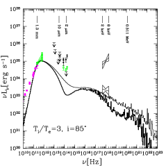
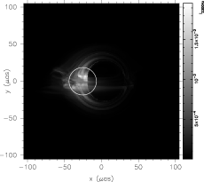
Figure 2.: Left panel: SEDs computed based on a single time slice $t=1680GM/c^{3}$ (thick line) (see Figure 3 for the distributions of the physical variables corresponding to the same time) along with the time averaged spectrum (thin line) of our best-bet model. Observational points are taken from: Falcke et al. 1998, An et al. 2005, Marrone et al. 2006 at radio, Genzel et al. 2003 at NIR (1.65, 2.16, and 3.76 ${\rm\mu m}$) and Baganoff et al. 2003 at X-rays (2-8 keV). The upper limits in the NIR band are taken from Melia & Falcke 2001 (30, 24.5 and 8.6 ${\rm\mu m}$), Schödel et al. 2007 (8.6 $\mu m$) and Hornstein et al. 2007 (2 ${\rm\mu m}$). The points in the NIR at flaring state are from Genzel et al. 2003 (1.65, 2.16, and 3.76 ${\rm\mu m}$) , and Dodds-Eden et al. 2009 (3.8 ${\rm\mu m}$). An example of X-ray flare ($L_{X}=1\times 10^{35}$ $ergs^{-1}$) is taken from Baganoff et al. 2001. Right panel: corresponding to SED in the left panel Image of the accretion flow at $230GHz$ correspindign to $t=1680GM/c^{3}$. Intensities are given in units of $ergs^{-1}{\rm pixelsize^{-2}Hz^{-1}sr^{-1}}$, where the pixel size is $0.82\mu as$. The image shows inner $40GM/c^{2}$. The white circle marks FWHM=37 $\mu as$ of a symmetric Gaussian brightness profile centered at the image centroid.

In Figure 3, we show the dynamical model corresponding to our best-bet model. We show maps of number density density, magnetic field strength and electron temperature ($\theta_{e}=k_{b}T_{e}/m_{e}c^{2}$) on a single time slice.

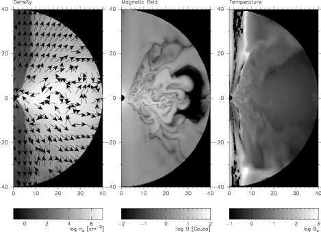
Figure 3.: Accretion flow structure in our best-bet model with $a_{*}=0.94$ and with $T_{i}/T_{e}=3$ (model D3). The number density overplotted with the velocity field, the magnetic field strength, and the electron temperature are shown in the left, middle, and right panel respectively. The axis units are $GM/c^{2}$.The figure shows a single time slice.

Figure 4 maps the points of origin for photons below and in the synchrotron peak (100-690 GHz), in the NIR ($10^{13}-10^{14}Hz$), and in the X-ray (2-8 keV). The figure again corresponds to a single time slice from our best-bet model presented in Figures 2, 3. Most of the submillimeter emission originates near the mid plane at $4<rc^{2}/(GM)<6$. NIR photons are produced in the hot regions close to the innermost circular orbit ($r_{ISCO}\approx 2.04GM/c^{2}$). Photons in the X-ray band are produces mainly by scatterings in the hottest parts of the disk also close to the $r_{ISCO}$. A small fraction of photons are emitted from the funnel wall at large radii ($15-40GM/c^{2}$).

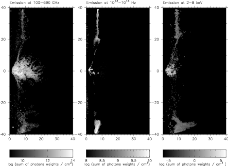
Figure 4.: Maps showing the point of origin for photons in our best-bet model. We show the logarithm of the sum of the photon weights in each zone, which is proportional to the number of photons seen at $100-690GHz$ (left), $10^{13}-10^{14}Hz$ (middle) and 2-8 keV (right) band. The axis scale units are $GM/c^{2}$. The figure presents a single time slice at $t=1680GM/c^{3}$. Note that gray scale bands differ in scales.

Summary of parameter survey

We can draw the following general conclusions from our work: (1) Very few of the time averaged SEDs based on a single-temperature ($T_{i}/T_{e}=1$) models produce the correct spectral slope between 230-690 GHz. The exception is edge-on tori ($i=85^{\hbox{${}^{\circ}$}}$) around a fast spinning black hole ($a_{*}=0.98,0.96$), but these models overproduce NIR and X-ray flux.

(2) For $T_{i}/T_{e}=3$ the only one model with $a_{*}=0.94$ at $i=85^{\hbox{${}^{\circ}$}}$ is consistent with all observational constraints. For $i=85\hbox{${}^{\circ}$}$, models with spins below $a_{*}=0.94$ are ruled out by the inconsistent spectral slope, and models with higher spins ($a_{*}>0.94$), although consistent with the observed $\alpha$, overproduce the quiescent NIR and X-ray emission. All models with $T_{i}/T_{e}=3$ observed at $i=5^{\hbox{${}^{\circ}$}}$ and $45^{\hbox{${}^{\circ}$}}$ are ruled out by the inconsistent $\alpha$.

(3) For $T_{i}/T_{e}=10$, we find that all models with $i=85^{\hbox{${}^{\circ}$}}$ are ruled out by both incorrect $\alpha$ and violation of NIR and X-ray limits. For lower inclination angles ($i=5^{\hbox{${}^{\circ}$}},45^{\hbox{${}^{\circ}$}}$) a few models (E10 and F10 with $i=5\hbox{${}^{\circ}$}$, and A10, B10, C10, and D10 at $i=45\hbox{${}^{\circ}$}$) reproduce the observed $\alpha$. These models are consistent with X-rays and NIR limitations. Models E and F for $i=45\hbox{${}^{\circ}$}$ are ruled out by NIR and X-ray limitations whereas models A10, B10, C10 and D10 for $i=5\hbox{${}^{\circ}$}$ produce $\alpha$ which is too small.

(4) The dependence on $a_{*}$ arises largely because as $a_{*}$ increases the inner edge of the disk — the ISCO – reaches deeper into the gravitational potential of the black hole, where the temperature and magnetic field strength are higher. In the disk mid-plane, the temperature is proportional to the virial temperature and scales with radius $\Theta_{e}\propto 1/r$. $B\propto 1/r$, while the density $\sim r$, below the pressure maximum (longer simulations in 3D show a more relaxed, declining density profile). Holding all else constant this implies a higher peak frequency for synchrotron emission, a constant Thomson depth (in our models the Thomson depth at the ISCO is roughly constant, since the path length $1/\sim r_{ISCO}$ but the density $\sim r_{ISCO}$), and a larger energy boost per scattering $A\approx 16\Theta_{e}^{2}$, as can be seen in comparing models with different spin in Figure 4. The X-ray flux therefore increases with $a_{*}$ because $\Theta_{e}$ at the ISCO increases.

(5) The dependence on $T_{i}/T_{e}$ is mainly due to synchrotron self-absorption, which is strongest at high inclination. For example, because the $i=85^{\hbox{${}^{\circ}$}}$, $T_{i}/T_{e}=10$ model is optically thick at $230GHz$ the emission is produced in a synchrotron photosphere well outside $r_{ISCO}$. The typical radius of the synchrotron photosphere ranges between 15 $GM/c^{2}$ for low spin models ($a_{*}=0.5,0.75$) and 8 $GM/c^{2}$ for high spin models ($a_{*}>0.75$). The $230GHz$ flux can then be produced only with large ${\mathcal{M}}$; as ${\mathcal{M}}$ increases the optically thin flux in the NIR increases due to increasing density and field strength. The scattered spectrum also depends on $T_{i}/T_{e}$ since the energy boost per scattering is $\sim 16\Theta_{e}^{2}\propto 1/(T_{i}/T_{e})^{2}$.

(6) The inclination dependence is a relativistic effect. ${\mathcal{M}}$ is nearly independent of $i$ (it varies by $\sim 10\%$, except for $T_{i}/T_{e}=10$, which due to optical depth effects has much larger variation), so models with different inclination are nearly identical. Nevertheless the X-ray flux varies dramatically with $i$, increasing by almost 2 orders of magnitude from $i=5\hbox{${}^{\circ}$}$ to $i=85^{\hbox{${}^{\circ}$}}$. This occurs because Compton scattered photons are beamed forward parallel to the orbital motion of the disk gas. The variation of mm flux with $i$ is due to self-absorption. The mm flux reflects the temperature and size of the synchrotron photosphere. At lower $i$ the visible synchrotron photosphere is hotter than at high $i$.

4. Future prospects

We have made a number of approximations that will be removed in future models of Sgr A*. We plan to (1) add cooling, (2) run 3D (rather than axisymmetric) models, (3) model a larger range of radii, (4) include a population of nonthermal electrons, (5) eliminate the fast-light approximation by doing fully time-dependent radiative transfer.

Acknowledgments.

This work was supported by the National Science Foundation under grants AST 00-93091, PHY 02-05155, and AST 07-09246, by NASA grant NNX10AD03G, through TeraGrid resources provided by NCSA and TACC, and by a Richard and Margaret Romano Professorial scholarship, a Sony faculty fellowship, and a University Scholar appointment to CFG.

References

- Abramowicz et al. (1978) Abramowicz, M., Jaroszynski, M., Sikora, M., & Sikora, M. 1978, A&A, 63, 221
- An et al. (2005) An, T., Goss, W. M., Zhao, J.-H., Hong, X. Y., Roy, S., Rao, A. P., & Shen, Z.-Q. 2005, ApJ, 634, L49
- Baganoff et al. (2001) Baganoff, F. K., Bautz, M. W., Brandt, W. N., Chartas, G., Feigelson, E. D., Garmire, G. P., Maeda, Y., Morris, M., Ricker, G. R., Townsley, L. K., & Walter, F. 2001, Nat, 413, 45
- Baganoff et al. (2003) Baganoff, F. K., Maeda, Y., Morris, M., Bautz, M. W., Brandt, W. N., Cui, W., Doty, J. P., Feigelson, E. D., Garmire, G. P., Pravdo, S. H., Ricker, G. R., & Townsley, L. K. 2003, ApJ, 591, 891
- Broderick et al. (2009) Broderick, A. E., Fish, V. L., Doeleman, S. S., & Loeb, A. 2009, , ApJ, 697, 45
- Broderick & Loeb (2005) Broderick, A. E. & Loeb, A. 2005, MNRAS, 363, 353
- Broderick & Loeb (2006a) —. 2006a, ApJ, 636, L109
- Broderick & Loeb (2006b) —. 2006b, MNRAS, 367, 905
- Chan et al. (2009) Chan, C.-k., Liu, S., Fryer, C. L., Psaltis, D., Özel, F., Rockefeller, G., & Melia, F. 2009, ApJ, 701, 521
- Dexter et al. (2009) Dexter, J., Agol, E., & Fragile, P. C. 2009, ApJ, 703, 142
- Dodds-Eden et al. (2009) Dodds-Eden, K., Porquet, D., Trap, G., Quataert, E., Haubois, et al. 2009, ApJ, 698, 676
- Doeleman et al. (2008) Doeleman, S. S., Weintroub, J., Rogers, A. E. E., Plambeck, R., Freund, R., et al. 2008, Nat, 455, 78
- Dolence et al. (2009) Dolence, J. C., Gammie, C. F., Mościbrodzka, M., & Leung, P. 2009, ApJ, 1, 1
- Falcke et al. (1998) Falcke, H., Goss, W. M., Matsuo, H., Teuben, P., Zhao, J.-H., & Zylka, R. 1998, ApJ, 499, 731
- Fishbone & Moncrief (1976) Fishbone, L. G. & Moncrief, V. 1976, ApJ, 207 , 962
- Gammie et al. (2003) Gammie, C. F., McKinney, J. C., & Tóth, G. 2003, ApJ, 589, 444
- Genzel et al. (2003) Genzel, R., Schödel, R., Ott, T., Eckart, A., Alexander, T., Lacombe, F., Rouan, D., & Aschenbach, B. 2003, Nat, 425, 934
- Ghez et al. (2008) Ghez, A. M., Salim, S., Weinberg, N. N., Lu, J. R., Do, T., Dunn, J. K., Matthews, K., Morris, M. R., Yelda, S., Becklin, E. E., Kremenek, T., Milosavljevic, M., & Naiman, J. 2008, ApJ, 689, 1044
- Gillessen et al. (2009) Gillessen, S., Eisenhauer, F., Trippe, S., Alexander, T., Genzel, R., Martins, F., & Ott, T. 2009, ApJ, 692, 1075
- Goldston et al. (2005) Goldston, J. E., Quataert, E., & Igumenshchev, I. V. 2005, ApJ, 621, 785
- Hilburn et al. (2009) Hilburn, G., Liang, E., Liu, S., & Li, H. 2009, arXiv/0909.4780
- Hornstein et al. (2007) Hornstein, S. D., Matthews, K., Ghez, A. M., Lu, J. R., Morris, M., Becklin, E. E., Rafelski, M., & Baganoff, F. K. 2007, ApJ, 667, 900
- Huang et al. (2007) Huang, L., Cai, M., Shen, Z.-Q., & Yuan, F. 2007, MNRAS, 379, 833
- Huang et al. (2009) Huang, L., Takahashi, R., & Shen, Z.-Q. 2009, ApJ, 706, 960
- Loeb & Waxman (2007) Loeb, A., & Waxman, E. 2007, J. Cosmol. Astropart. Phys, 03, 011
- Markoff et al. (2001) Markoff, S., Falcke, H., Biermann, P.L., & Yuan, F. 2001, A&A, 379, L13
- Markoff et al. (2007) Markoff, S., Bower, C.B., & Falcke, H. 2007, MNRAS, 379, 1519
- Marrone (2006) Marrone, D. P. 2006, PhD thesis, Harvard University
- Marrone et al. (2006) Marrone, D. P., Moran, J. M., Zhao, J.-H., & Rao, R. 2006, Journal of Physics Conference Series, 54, 354
- McKinney & Gammie (2004) McKinney, J. C. & Gammie, C. F. 2004, ApJ, 611, 977
- Melia & Falcke (2001) Melia, F. & Falcke, H. 2001, ARA&A, 39, 309