Metal-Ion Absorption in Conductively Evaporating Clouds

Abstract

We present computations of the ionization structure and metal-absorption properties of thermally conductive interface layers that surround evaporating warm spherical clouds, embedded in a hot medium. We rely on the analytical steady-state formalism of Dalton and Balbus to calculate the temperature profile in the evaporating gas, and we explicitly solve the time-dependent ionization equations for H, He, C, N, O, Si, and S in the conductive interface. We include photoionization by an external field. We estimate how departures from equilibrium ionization affect the resonance-line cooling efficiencies in the evaporating gas, and determine the conditions for which radiative losses may be neglected in the solution for the evaporation dynamics and temperature profile. Our results indicate that non-equilibrium cooling significantly increases the value of the saturation parameter $\sigma_{0}$ at which radiative losses begin to affect the flow dynamics. As applications we calculate the ion fractions and projected column densities arising in the evaporating layers surrounding dwarf-galaxy-scale objects that are also photoionized by metagalactic radiation. We compare our results to the UV metal-absorption column densities observed in local highly-ionized metal-absorbers, located in the Galactic corona or intergalactic medium. Conductive interfaces significantly enhance the formation of high-ions such as C³⁺, N⁴⁺, and O⁵⁺ relative to purely photoionized clouds, especially for clouds embedded in a high-pressure corona. However, the enhanced columns are still too low to account for the O VI columns ($\sim 10^{14}$ cm^-2) observed in the local high-velocity metal-ion absorbers. We find that column densities larger than $\sim 10^{13}$ cm^-2 cannot be produced in evaporating clouds. Our results do support the conclusion of Savage and Lehner, that absorption due to evaporating O VI likely occurs in the local interstellar medium, with characteristic columns of $\sim 10^{13}$ cm^-2.

1. Introduction

The physics of conductively evaporating clouds has applications to a variety of astrophysical environments. This includes the study of the Local Cloud and Local Bubble (Slavin 1989; Smith & Cox 2001, Slavin & Frisch 2002; Savage & Lehner 2006; Jenkins 2009), cloud evaporation in the interstellar medium (e.g. B$\ddot{\rm o}$hringer & Hartquist 1987; Dalton & Balbus 1993; Nagashima et al. 2007; Slavin 2007; Vieser & Hensler 2007), supernovae remnants (e.g. Shelton 1998; Slavin & Cox 1992; Balsara et al. 2008), active galactic nuclei (e.g. McKee & Begelman 1990), and the galaxy formation process (Nipoti & Binney 2007).

In this paper, we present new computations of the non-equilibrium ionization states and metal absorption line signatures of thermally conductive interfaces that surround evaporating warm ($\sim 10^{4}$ K) spherical gas clouds embedded in a hot ionized medium (HIM, $\gtrsim 10^{6}$ K). In such interfaces, the warm clouds undergo steady evaporation, while heat from the hot ambient medium flows into the clouds (Cowie & McKee 1977; McKee & Cowie 1977). We compute the integrated metal-ion column densities through the conductive interfaces, for comparison to absorption line observations. We consider the effect of photoionization by the metagalactic radiation field on the non-equilibrium ionization states in the conduction fronts.

As matter flows from the warm cloud toward the hot ambient medium, its ionization state changes continuously. Non-equilibrium effects become significant when the ionization time-scale is long compared to the rate of temperature change. The gas then tends to remain “underionized” compared to gas in ionization equilibrium at the same temperature. Because the energy losses in the evaporating gas are dominated by atomic and ionic line emissions from many species, the cooling efficiencies are affected by the non-equilibrium abundances. For underionized gas, cooling is enhanced.

Our theoretical work is motivated by recent ultraviolet and X-ray absorption line spectroscopy of hot gas in the Galactic halo, around higher redshift galaxies, and in intergalactic environments (e.g. Sembach et al. 2003; Collins et al. 2005; Savage et al. 2005; Tumlinson et al. 2005; Fang et al. 2006; Stocke et al. 2006; Narayanan et al. 2010). We are also motivated by observations of discrete ionized “high-velocity clouds” (Sembach et al. 1999, 2000, 2002, 2003; Murphy et al. 2000; Wakker et al. 2003; Collins et al. 2003, 2004, 2007; Fox et al. 2005, 2006). These observations indicate that the ionized gas is not in equilibrium ionization (Sembach et al. 2002; Fox et al. 2004, 2005; Gnat & Sternberg 2004), and non-equilibrium processes such as time-dependent radiative cooling (e.g. Gnat & Sternberg 2007; Sutherland & Dopita 1993), shock ionization (e.g. Allen et al. 2008; Gnat & Sternberg 2009), or ionization in conductive interfaces (this paper) may be at play in these objects.

Theoretical models of cloud evaporation in a hot medium have been studied extensively. Cowie & McKee (1977) developed an analytical solution for the mass loss rate and temperature profile in static conductive interfaces around spherical clouds. In their solution, they included the possible effects of heat flow saturation that occurs when the electron mean free path is not small compared to the temperature scale height (see §2). The saturation in the flow can be measured by one global parameter, the “saturation parameter” $\sigma_{0}$. McKee & Cowie (1977) studied the effects of radiative losses on the interface. In particular, they demarcated the range of saturation parameters for which radiative losses may be neglected. The situation becomes much more complicated if the dynamics of the evaporation are affected by magnetic fields (e.g. Slavin 1989; Borkowski, Balbus & Fristrom 1990) or if the evaporation is time-dependent (e.g. Shelton 1998; Smith & Cox 2001; Vieser & Hensler 2007).

Non-equilibrium ionization in conductive interfaces was considered previously in several studies (Ballet, Arnaud & Rothenflug 1986; B$\ddot{\rm o}$hringer & Hartquist 1987; Dalton & Balbus 1993; Slavin 1989; Slavin & Cox 1992; Shelton  1998; Smith & Cox 2001). However, most of these works explored only a limited range of parameters (with $P_{\rm HIM}/k_{\rm B}\sim 10^{4}$ cm^-3 K and $R_{\rm cloud}\sim 1$ pc), appropriate for interstellar clouds. None of the previous computations included photoionization by an external radiation field.

Here we calculate the ion fractions created in the conductive interfaces surrounding evaporating gas clouds. We consider pressures between $0.1$ and $10^{4}$ cm^-3 K, cloud radii between $1$ pc and $100$ kpc, and ambient temperatures between $5\times 10^{5}$ K and $10^{7}$ K. We study how the metal absorption line properties depend on the interface parameters. We consider the effects of non-equilibrium cooling and reexamine the criterion derived by McKee & Cowie (1977) for the neglect of radiative losses in the evaporative flows.

As applications, we then focus on the example of the local “ionized high-velocity clouds”. Over the past decade, UV absorption line observations have revealed a population of local high-velocity metal-ion absorbers (Sembach et al. 1999, 2000, 2002, 2003; Murphy et al. 2000; Wakker et al. 2003; Collins et al. 2004; Fox et al. 2005, 2006). The observations, carried out with the Goddard High Resolution Spectrometer (GHRS) and Space Telescope Imaging Spectrograph (STIS) on board HST, and more recently with the Far Ultraviolet Spectroscopic Explorer (FUSE), indicate the presence of many high-ionization metal absorption lines, including Si III $\lambda~{}1206.5$, Si IV $\lambda\lambda~{}1393.8,~{}1402.8$, and C IV $\lambda\lambda~{}1548.2,~{}1550.8$ with little or no associated H I (N${}_{\rm{HI}}\lesssim 10^{15}-10^{16}$ cm^-2). Of particular interest is O VI $\lambda~{}1031.9$, for which absorbing column densities of order $10^{14}$ cm^-2 have been measured (Collins et al. 2004; Fox et al. 2006; Sembach et al. 2000, 2003).

Many of these ionized absorbers can be identified with the diffuse nearby H I high-velocity cloud complexes, such as the Magellanic Stream or Complex C (Sembach et al. 2003). However, some of these absorbers do not appear directly linked to such structures, and could be clouds at much larger distances, perhaps pervading the Local Group. The absorbers towards Mrk 509 and PKS 2155-304 are examples of such isolated high-velocity metal-ion absorbers (Sembach et al. 1999; Collins et al. 2004; Fox et al. 2005). As a guide to these observations, we list in Table 1 the data presented by Collins et al. (2004) for the metal-ion absorbers towards Mrk 509.

In Gnat & Sternberg (2004, hereafter GS04), we modeled the high-velocity metal ion absorbers as photoionized gas clouds associated with low-mass dark matter “minihalos” (see also Kepner et al. 1999). For this purpose, we studied the metal photoionization properties of hydrostatic gas clouds embedded in gravitationally dominant dark-matter halos, that are photoionized by the present-day cosmological metagalactic radiation field, and are pressure-confined by an external hot medium. We considered minihalo models for dwarf-galaxy-scale objects and for the lower mass compact H I high velocity clouds (CHVCs), based on the properties derived by Sternberg, McKee, & Wolfire (2002; see also Giovanelli et al. 2010).

For low mass objects ($M_{\rm vir}\sim 10^{8}$ M_⊙) embedded in the relatively high-pressure environment of the Galactic corona ($P\sim 50$ cm^-3 K), we found that the ionization parameter is too low to efficiently produce C IV and other high ions. However, for the more massive dwarf-galaxy-scale halos ($M_{\rm vir}\sim 2\times 10^{9}$ M_⊙, $P\lesssim 1$ cm^-3 K) embedded in the low-pressure intergalactic medium (IGM), we found that their ionized envelopes are natural sites for the formation of high-ions. Photoionized envelopes of dwarf-galaxy-scale halos could be detectable as UV metal-line absorbers, with ionization states similar to those observed in the ionized high-velocity absorbers. O VI remains an important exception, as it is inefficiently produced by photoionization.

The strong O VI absorption in the high-velocity metal-ion absorbers strongly suggests that photoionization is not the only ionization mechanism at play in these objects (Sembach et al. 1999; Fox et al. 2004, 2005; GS04). The contribution of additional ionization processes may produce high-ions that are suppressed in the purely photoionized clouds.

The fact that minihalo clouds may be embedded in a hot plasma, such as the Galactic corona or the intergalactic medium at various redshifts, suggests the possibility of significant collisional interactions between the hot gas and the warm clouds. Here we use our evaporating cloud models to study the interface layers surrounding dwarf-galaxy-scale minihalos ($0.1<P/k_{\rm B}<50$ cm^-3 K, $R_{\rm cloud}\sim$ kpc, $T_{\rm HIM}\gtrsim 10^{6}$ K, $Z=0.1$ solar) for comparison with the observations of the high-velocity metal ion absorbers. As we describe below, we include the effect of photoionization by the metagalactic external radiation on the non-equilibrium ionization properties of the gas in the interface.

In §2 we describe the basic equations and numerical method. In §3 we present a set of computations of the ion fractions in conductive interfaces, and we discuss the resulting metal absorption column densities for the dwarf-galaxy-scale models in §4. We find that conductive interfaces significantly enhance the formation of high ions such as C³⁺, N⁴⁺ and O⁵⁺ relative to purely photoionized clouds, especially for clouds embedded in a high-pressure medium. However, the enhanced columns are still too low to account for the O VI columns ($\sim 10^{14}$ cm^-2) observed in the high-velocity metal-ion absorbers. We find that O VI column densities larger than $\sim 10^{13}$ cm^-2 cannot be produced in evaporating clouds. Our models do support the conclusion by Savage & Lehner (2006) that evaporating O VI absorption occurs in the local ISM, with characteristic columns of $\sim 10^{13}$ cm^-2. We summarize in §5.

Table 1Column-Density Measurements in MrK 509

Ion	-300 km s-1	-240 km s-1
C II	$4.79^{+0.97}_{-0.90}\times 10^{13}$	$<2.09\times 10^{13}$
N I	$<3.39\times 10^{13}$	$<2.40\times 10^{13}$
Si II	$<1.23\times 10^{12}$	$8.51^{+2.05}_{-1.33}\times 10^{12}$
S II	$<1.00\times 10^{14}$	$<7.08\times 10^{13}$
C IV	$1.41^{+0.37}_{-0.21}\times 10^{14}$	$3.39^{+0.41}_{-0.44}\times 10^{13}$
N V	$<1.74\times 10^{13}$	$<1.20\times 10^{13}$
O VI	$8.51^{+0.82}_{-0.93}\times 10^{13}$	$7.76^{+0.75}_{-0.68}\times 10^{13}$
Si III	$2.04^{+0.15}_{-0.18}\times 10^{13}$	$2.75^{+0.71}_{-0.66}\times 10^{12}$
Si IV	$3.39^{+1.86}_{-0.88}\times 10^{13}$	$<3.09\times 10^{12}$
S III	$<8.51\times 10^{13}$	$<6.03\times 10^{13}$

Note. — Column densities for two velocity components toward Mrk 509 by Collins et al. (2004). The error estimates are the $1\sigma$ estimates, and the upper limits are $3\sigma$ limits.

2. Basic Equations and Processes

2.1. Evaporation

We are interested in studying the evolving non-equilibrium ionization states in thermally conductive gas that evaporates from warm purely photoionized clouds into a hot ambient medium. In our treatment of the ionization in the evaporating layers we use an analytic solution for the temperature profiles in the conductive interfaces surrounding steady-state, spherical, non-magnetic clouds. The temperature profiles are obtained by solving the equation of energy conservation in the flow, balancing the outward energy flux with the inward heat flux. Within the interface, the heat flux changes from a classical diffusive form,

$$\mathbf{q}_{\rm cl}=-\kappa\nabla T$$ (1)

(Spitzer 1962) that applies when the electron mean free path is small compared to the temperature scale height ($T/\nabla T$), to a saturated form,

$$|\mathbf{q}_{\rm sat}|=5\phi_{s}\rho c^{3}$$ (2)

(Cowie & McKee 1977) when the mean free path is comparable to, or greater than, the temperature scale height. In the above expressions, $\kappa$ is the thermal conductivity, $\rho$ is the mass density, $c$ is the sound speed, and $\phi_{s}$ is a factor of order unity that allows for various uncertainties in the estimation of $q_{\rm sat}$.

The local saturation in the flow is defined by the ratio (Cowie & McKee 1977),

$$\sigma=\frac{q_{\rm cl}}{q_{\rm sat}}\;,$$ (3)

and is proportional to the ratio of the mean free path to the temperature scale height.

For a classical diffusive interface, the rate of mass loss

$$\dot{m}_{\rm cl}=\frac{16\pi\mu R\kappa_{\rm HIM}}{25k_{\rm B}}$$ (4)

(Cowie & McKee 1977), where $R$ is the cloud radius, $\mu$ is the mean mass per particle, $k_{B}$ is the Boltzmann constant, and subscript “HIM” refers to the surrounding hot ionized medium. As the flow saturates, the heat flux is limited to a maximal rate given by equation (2), and the classical mass loss rate is reduced by a factor $\omega$ such that $\dot{m}=\omega\dot{m}_{\rm cl}$. The global level of saturation in the flow is parametrized by the saturation parameter,

$$\sigma_{0}\equiv\frac{2\kappa_{\rm HIM}T_{\rm HIM}}{25\phi_{s}\rho_{\rm HIM}c_{\rm HIM}^{3}R}\propto\frac{T_{\rm HIM}^{2}}{\rho_{\rm HIM}R}\propto\frac{T_{\rm HIM}^{3}}{PR}\;$$ (5)

(Cowie & McKee 1977). In this expressions $T$ is the temperature, and $P=\rho k_{\rm B}T/\mu$ is the gas pressure.

To obtain the steady state temperature profile in the conductive interface, the equation of energy conservation,

$$\nabla\cdot\left[\frac{\rho\mathbf{v}}{2}(\mathbf{v}^{2}+5c^{2})\right]+\left(n^{2}\Lambda-n\Upsilon\right)=-\nabla\cdot\mathbf{q}$$ (6)

must be solved, where $\Lambda$ is the cooling efficiency (erg cm³ s^-1), and $\Upsilon$ is the heating rate (erg s^-1). The first term on the left hand side of equation (6) is a bulk kinetic energy term; the second is due to internal energy and $PdV$ work; and the next two terms account for radiative losses (cooling) and gains (heating). This outward energy flux is balanced by an inward heat flux represented by the right hand side of equation (6).

We rely on the formalism developed by Dalton & Balbus (1993, hereafter DB93) for determining the temperature profile in the interface. The DB93 formalism allows the thermal conductivity to change continuously from the classical diffusive form to a saturated form, by using an effective heat flux $q$, defined as the harmonic mean of the local classical and saturated fluxes,

$$\frac{1}{q}\equiv\frac{1}{q_{\rm cl}}+\frac{1}{q_{\rm sat}}\;.$$ (7)

DB93 then solve for the steady state temperature profile that develops in the interface layer between the warm cloud and the hot medium surrounding it.

When solving the energy equation, DB93 neglect the kinetic energy term, as well as the radiative losses (cooling) term. We discuss both assumptions in detail below. With these simplifying assumptions, the equation of energy conservation becomes,

$$\nabla\cdot\left(\frac{5}{2}\rho\mathbf{v}c^{2}\right)=-\nabla\cdot\mathbf{q}\;.$$ (8)

The temperature profile in the conductive interface then depends only on the global saturation parameter, $\sigma_{0}$, which is a function of the cloud radius, and the ambient pressure and temperature, as given by equation (5). Temperature profiles for various values of $\sigma_{0}$ are shown in Figure 1.

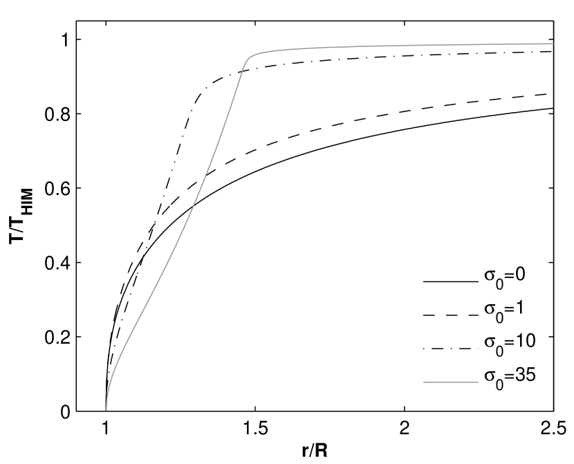
Figure 1.— Scaled temperature, $T/T_{\rm HIM}$ versus scaled distance $r/R$, computed using the DB93 analytical solutions, for a range of saturation parameters.

2.1.1 On the Validity of the Subsonic Approximation

The kinetic energy term may be neglected when $v^{2}\ll 5c^{2}$ (see equation 6), or equivalently when $M^{2}\ll 5$. If the kinetic energy is small relative to the internal energy, the flow is isobaric, with a constant gas pressure $P=\rho_{\rm HIM}k_{\rm B}T_{\rm HIM}/\mu$.

In classical flows, $M$ is always less than unity, and the subsonic approximation holds. However, as the flow saturates, the maximal Mach number increases. In fully saturated flows, the heat flux is given by equation (2), and equation (6) reads

$$5/2\;\;\rho vr^{2}c^{2}(1+M^{2}/5)-5\phi_{s}\rho c^{3}r^{2}=0,$$ (9)

This implies that in fully saturated flows

$$M(1+M^{2}/5)=2\phi_{s}$$ (10)

(e.g. Cowie & McKee 1977). Therefore, for $\phi_{s}<0.6$, the subsonic approximation holds throughout the flow.

As a consistency check, we also consider the local Mach number in the analytic profiles derived by Dalton & Balbus neglecting the kinetic energy term. In this case

$$M=T^{1/2}\frac{k_{\rm B}}{P}\frac{\omega}{4\pi r^{2}}\left(\frac{16\pi\mu^{1/2}\kappa_{\rm HIM}R}{25k_{\rm B}^{3}}\right)$$ (11)

(DB93 equation B3). Given a set of temperature profiles appropriate for a range of saturation parameters (see Figure 1), this equation shows that the maximal Mach number is an increasing  function of $\sigma_{0}$. With the kinetic energy term neglected, the maximal Mach number approaches $2\phi_{s}$ in highly saturated flows, implying that for $\phi_{s}<0.5$ the subsonic approximation holds even for large $\sigma_{0}$.

Experimental evidence suggests that $\phi_{s}\sim 0.3$ (see Balbus & McKee 1982). Throughout this paper we therefore assume $\phi_{s}=0.3$, consistent with the use of subsonic approximation.

2.1.2 On the Validity of the Non-Radiative Approximation

The fate of warm clouds that are embedded in a hot ambient medium depends of the delicate balance between the conductive heating and the radiative losses in the interface. Evaporation takes place if the radiative losses are small compared to conductive heating. If, on the other hand, cooling overcomes the conductive heating, the evaporation stops, and instead the ambient medium condenses onto the warm cloud.

McKee & Cowie (1977) used an approximate analytical method to determine the critical cloud radii at which radiative losses balance the conductive heating. They used fits to the equilibrium cooling functions of solar metallicity gas to derive these critical radii as a function of the external temperature and density. McKee & Cowie found that radiative losses are important only at low saturations, $\sigma_{0}\lesssim 0.03/\phi_{s}$. Such small values of $\sigma_{0}$ are generally out of the regime “occupied” by dwarf-galaxy scale halos (for which $\sigma_{0}>0.2$).

Our models differ from those presented by McKee & Cowie. First, we explicitly follow the non-equilibrium ion fractions in the interface. As mentioned above, the outflowing gas may be underionized relative to gas in equilibrium at the same temperature. Underionized gas tends to radiate more efficiently (McCray 1987; Gnat & Sternberg 2007), thus increasing the contributions of radiative losses. Second, we include photoionization by an external background radiation field. This both increases the ionization level in the gas and provides heating, both effects acting to reduce the importance of radiative losses. Finally, we assume gas metallicity of $0.1$ solar, thus reducing the cooling efficiency. The relative importance of these three effects must be estimated numerically.

Using our numerical results we check, for each model, whether the emissivity associated with the heat flux is indeed everywhere larger than the radiative cooling. Given our non-equilibrium ion fractions (including photoionization, see section 2.2), we use the cooling functions included in Cloudy (version 07.02, Ferland et al. 1998) to compute the local cooling efficiencies. We then compare these values with $\nabla\cdot\mathbf{q}$.

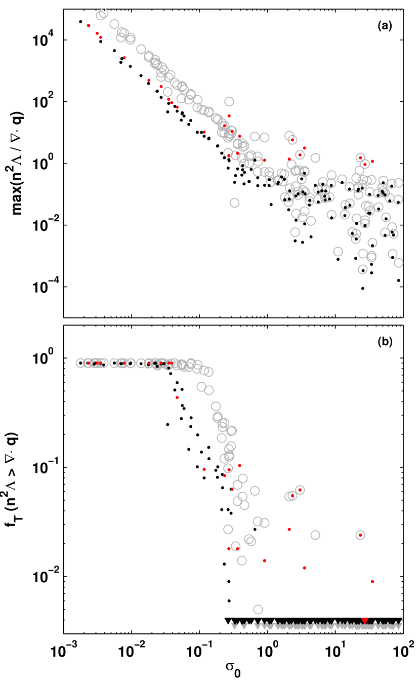
Figure 2.— (a) Maximum of $n^{2}\Lambda/\nabla\cdot\mathbf{q}$ versus saturation parameter $\sigma_{0}$. The black ($P/k_{\rm B}\leq 10^{3}$ cm^-3 K) and red ($P/k_{\rm B}=10^{4}$ cm^-3 K) points are for $Z=0.1$ solar metallicity gas. For $P/k_{\rm B}=10^{4}$ cm^-3 K the neutral fraction on the cloud surface is considerable ($x_{\rm HI}=0.574$). The gray circles are for solar metallicity gas (all pressures). (b) Fraction of interface temperature range over which the cooling is locally larger than $\nabla\cdot\mathbf{q}$. Triangles indicate models for which this fraction is smaller than $0.003$.

Figure 2 displays our results. Panel (a) shows the maximal ratio of the radiative to conductive emissivity in each model as a function of the saturation. Panel (b) shows the fraction of the interface temperature over which the cooling is larger than the conductive heating as a function of saturation. The points (black and red) are for our assumed heavy element abundances of $Z=0.1$ times solar. The gray circles show results for solar metallicity gas, for a direct comparison with the critical $\sigma_{0}$ derived by McKee & Cowie (1977).

For $Z=0.1$ times solar, both panels show that for $\sigma_{0}\lesssim 0.2$ (for $\phi_{s}=0.3$) radiative losses are significant and may not be neglected. For larger values of $\sigma_{0}$ the importance of radiative cooling is generally smaller, and depends on the specific parameters of the evaporating cloud.

For $\sigma_{0}\gtrsim 0.2$, enhanced cooling and larger values of $n^{2}\Lambda/\nabla\cdot\mathbf{q}$ are associated with interfaces of higher gas densities, with larger neutral fractions at the cloud surface. We find that for our assumed $10^{4}$ K-photoionized clouds, the neutral fraction on the surface is significant when $P\gtrsim 10^{4}$ cm^-3 K. For example, for pressures of $P=10^{4}$, $10^{3}$, and $100$ cm^-3 K, the neutral fractions are $0.57$, $0.20$, and $0.03$, respectively. Neutral gas cools very efficiently, and in underionized flows the lingering and enhanced contribution of H I Ly$\alpha$ cooling significantly affects the energy balance.

To study the impact of the surface ionization on the flow dynamics, we distinguish between “neutral cloud” models for which $P/k_{\rm B}\gtrsim 10^{4}$ cm^-3 K (red points), and “ionized cloud” models with $P/k_{\rm B}\leq 10^{3}$ cm^-3 K (black points). Figure 2 shows that for $\sigma_{0}\gtrsim 0.2$, radiative losses are negligible for bounding pressures $\leq 10^{3}$ cm^-3 K. However, in more neutral clouds cooling may be significant even at high saturations.

The fact that the limiting saturation parameter that we find is similar to the one derived by McKee & Cowie (1977, $\sigma_{0}=0.03/\phi_{s}$) – despite the $10$ times lower metallicity that we use, and the inclusion of photoionization – implies that the cooling efficiencies in our non-equilibrium interfaces are considerably larger than their equilibrium counterparts. In fact, we find that Ly$\alpha$ from underionized He⁺ dramatically increases the cooling efficiency in the interface. We discuss this point in detail in section 3.

For $Z=1$ solar, we find that radiative losses are important up to a critical saturation parameter of $\sigma_{0}\sim 0.5$ (for $\phi_{s}=0.3$), and become less significant for larger values of $\sigma_{0}$. Since underionized He⁺ is one of the dominant coolants in the interface, increasing the metallicity from a tenth-solar to solar changes the critical saturation parameter by a factor smaller than $10$. Figure 2 shows that this factor is $\sim 3$.

For the tenth solar metallicity dwarf-galaxy-scale models that we use for comparison with the observations of the high-velocity metal-ion absorbers, the radiative losses are, in fact, everywhere smaller than the conductive heating.

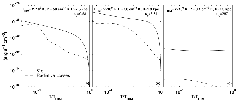
Figure 3.— Comparison of the radiative losses and $\nabla\cdot\mathbf{q}$ (erg s^-1 cm^-3), for three interface models, with $\sigma_{0}$ of $3.34$ (a), $0.58$ (b), and $267$ (c).

Some examples are shown in Figure 3, in which we compare $\nabla\cdot\mathbf{q}$ (solid curves) with the radiative losses (dashed curves) in three interface models. The left hand panels are for interfaces embedded in a high pressure corona, with $P/k_{\rm B}=50$ cm^-3 K. We show results for a small, marginally saturated cloud ($R=1.3$ kpc, $\sigma_{0}\sim 3$) in panel (a), and for a classical interface surrounding a larger cloud ($R=7.5$ kpc, $\sigma_{0}\sim 0.6$) in panel (b). In panel (c) we present a highly saturated interface, with $\sigma_{0}\sim 270$, surrounding a $7.5$ kpc cloud, embedded in a low pressure intergalactic medium ($P/k_{\rm B}=0.1$ cm^-3 K). In all cases, the radiative losses are everywhere smaller than the emissivity associated with the heat flux. These plots confirm that the significance of radiative losses is larger for lower saturation parameters, and becomes small at larger $\sigma_{0}$.

2.2. Ionization

Given the DB93 temperature profile, we solve for the non-equilibrium abundances of the various species in the interface. We follow the time-dependent ionization in the evaporating gas, given the initial photoionization equilibrium state in the warm cloud. We consider all ionization stages of the elements H, He, C, N, O, Si, and S. The temperature-dependent ionization and recombination processes that we include are collisional ionization by thermal electrons (Voronov 1997), radiative recombination (Aldrovandi & Pequignot 1973; Shull & van Steenberg 1982; Landini & Monsignori Fossi 1990; Landini & Fossi 1991; Pequignot, Petitjean, & Boisson 1991; Arnaud & Raymond 1992; Verner et al. 1996), dielectronic recombination (Aldrovandi & Pequignot 1973; Arnaud & Raymond 1992; Badnell et al. 2003, Badnell 2006; Colgan et al. 2003, 2004, 2005; Zatsarinny et al. 2003, 2004a, 2004b, 2005a, 2005b, 2006; Altun et al. 2004, 2005, 2006; Mitnik & Badnell 2004), and neutralization and ionization by charge transfer reactions with hydrogen and helium atoms and ions (Kingdon & Ferland fits, based on Kingdon & Ferland 1996, Ferland et al. 1997, Clarke et al. 1998, Stancil et al. 1998; Arnaud & Rothenflug 1985).

The time-dependent equations for the ion abundance fractions, $x_{i}$, of element $m$ in ionization stage $i$ are,

$$\begin{array}[]{l}v\;\;d{x_{i}}/dr=x_{i-1}~{}~{}[q_{i-1}n_{\rm e}+\Gamma_{i-1}+k^{\rm H}_{\uparrow i-1}n_{\rm H^{+}}\\ \;\;\;\;\;\;\;\;\;\;\;\;\;\;\;\;\;\;\;\;\;\;\;\;\;\;\;\;\;\;+k^{\rm He}_{\uparrow i-1}n_{\rm He^{+}}]\\ \;\;\;\;\;\;\;+x_{i+1}~{}~{}[\alpha_{i+1}n_{\rm e}+k^{\rm H}_{\downarrow i+1}n_{\rm H^{0}}+k^{\rm He}_{\downarrow i+1}n_{\rm He^{0}}]\\ \;\;\;\;\;\;\;-x_{i}~{}~{}[(q_{i}+\alpha_{i})n_{\rm e}+\Gamma_{i}+k^{\rm H}_{\downarrow i}n_{\rm H^{0}}+k^{\rm He}_{\downarrow i}n_{\rm He^{0}}\\ \;\;\;\;\;\;\;\;\;\;\;\;\;\;\;\;\;+k^{\rm H}_{\uparrow i}n_{\rm H^{+}}+k^{\rm He}_{\uparrow i}n_{\rm He^{+}}]\ \ \ .\end{array}$$ (12)

In this expression, $v$ is the gas velocity at radius $r$ in the evaporating flow. The parameters $q_{i}$ and $\alpha_{i}$ are the rate coefficients for collisional ionization and recombination (radiative plus dielectronic), and $k^{\rm H}_{\downarrow i}$, $k^{\rm H}_{\uparrow i}$, $k^{\rm He}_{\downarrow i}$, and $k^{\rm He}_{\uparrow i}$ are the rate coefficients for charge transfer reactions with hydrogen and helium that lead to ionization or neutralization. The quantities $n_{\rm H^{0}}$, $n_{\rm H^{+}}$, $n_{\rm He^{0}}$, $n_{\rm He^{+}}$, and $n_{\rm e}$ are the particle densities (cm^-3) for neutral hydrogen, ionized hydrogen, neutral helium, singly ionized helium, and electrons, respectively. $\Gamma_{i}$ are the photoionization rates of ions $i$, due to externally incident radiation.

For the external radiation, we use the Sternberg, McKee & Wolfire (2002) fit for the present-day metagalactic field,

$$J_{\nu}=\left\{\begin{array}[]{lcl}1.051\times 10^{2}J_{\nu 0}(\frac{\nu}{\nu_{0}})^{-1.5}&,&\frac{\nu}{\nu_{0}}~{}<~{}0.3\\ J_{\nu 0}(\frac{\nu}{\nu_{0}})^{-5.41}&,&0.3~{}<~{}\frac{\nu}{\nu_{0}}~{}<~{}1\\ J_{\nu 0}(\frac{\nu}{\nu_{0}})^{-3.13}&,&1~{}<\frac{\nu}{\nu_{0}}~{}<~{}4\\ 2.512\times 10^{-2}J_{\nu 0}(\frac{\nu}{\nu_{0}})^{-0.46}&,&4~{}<~{}\frac{\nu}{\nu_{0}}\\ \end{array}\right.$$ (13)

to compute $\Gamma_{i}$. In this expression $J_{\nu 0}=2\times 10^{-23}$ erg s^-1 cm^-2 Hz^-1 sr^-1, and $\nu_{0}$ is the Lyman limit frequency. This fit, which we plot in Figure 4, is based on observational constraints for the optical/UV and X-rays, (Bernstein et al. 2002; Martin et al. 1991; Chen et al. 1997) and on theoretical models (Haardt & Madau 1996) for the unobservable radiation from the Lyman limit to $\sim 0.25$ keV.

Recent observations and modeling have suggested that the spectral slope of the metagalactic radiation may be shallower near the Lyman limit, with $J_{\nu}$ varying as $\nu^{-1.8}$, and steepen gradually with increasing energy (e.g. Shull et al. 1999; Telfer et al. 2002; Scott et al. 2004; Shull et al. 2004; Zheng et al. 2004; Faucher-Giguere et al. 2009). In Appendix A we consider a radiation field (also plotted in Figure 4) that varies as $\nu^{-1.725}$ from the Lyman limit to $0.25$ keV, and investigate the sensitivity of our results to the spectral slope. For reference, we also plot in Figure 4 the Faucher-Giguere et al. (2009) model computation of the present-day metagalactic field. In Appendix A we show that the column densities of the high ions (O VI and N V) are insensitive to the spectral slope at the Lyman limit, while the column densities of lower ions (e.g. Si III) may be affected at a level of $<0.5$ dex, mostly for low external bounding pressures.

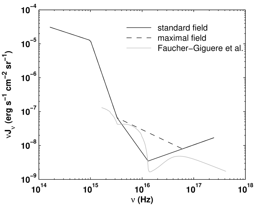
Figure 4.— The present-day metagalactic radiation field. The solid dark curve is for our standard field as represented by Sternberg et al. (2002; see text and Equation 13), the gray curve is for the Faucher-Giguere et al. (2009) field, and the dashed curve is for the shallower ”maximal field” considered in Appendix A (Gnat & Sternberg 2004).

The present-day metagalactic radiation field. The solid dark line is for the standard field as represented by Sternberg et al. (2002; see text and Equation 13), the gray line is for the Faucher-Giguere et al. (2009) field, and the dashed line is for the shallower ”maximal field” considered in Appendix A (Gnat & Sternberg 2004).

For each element $m$, the ion fractions $x_{i}\equiv n_{i,m}/(n_{\rm H}A_{m})$ satisfy

$$\sum x_{i}=1$$ (14)

where $n_{i,m}$ is the density (cm^-3) of ions in ionization stage $i$ of element $m$, $n_{\rm H}$ is total hydrogen density, and $A_{m}$ is the abundance of element $m$ relative to hydrogen. The sum is over all ionization stages of the element.

For the atomic elements that we include, equations (12) are a set of $54$ coupled ordinary differential equations (ODEs). For the initial conditions, we assume that the cloud surface is in photoionization equilibrium with the metagalactic filed, and has a temperature of $10^{4}$ K. We advance the solutions in small spatial steps $\Delta r$, where $r$ is the current distance from the cloud center ($r>R$), which is associated with a temperature $T(r)$ through the analytical solutions outlined by DB93. We integrate equations (12) over the interval $\Delta r$ using the same Livermore ODE solver (Hindmarsh 1983) we used in Gnat & Sternberg (2007). We verified that our code converges to the equilibrium abundances given a constant temperature, by comparing our solutions to those found by solving the set of algebraic equations for $x_{i}$ obtained by setting $dx_{i}/dr=0$ in equation (12), as appropriate for steady state. We verified our time-dependent computations by comparing with previous non-equilibrium models (e.g. Sutherland & Dopita 1993), as discussed in detail in Gnat & Sternberg (2007).

3. Metal Ions Fractions and Cooling in Evaporating Clouds

We computed the ionization states of the elements H, He, C, N, O, Si, and S in thermally conductive interfaces surrounding evaporating warm gas clouds. We calculate the non-equilibrium ionization states as a function of distance from the warm cloud surface. We consider a grid of models with pressures between $0.1$ and $10^{4}$ cm^-3 K, cloud radii between $1$ pc and $100$ kpc, and ambient (HIM) temperatures between $5\times 10^{5}$ and $10^{7}$ K. We assume heavy element abundance of $0.1$ times solar, as listed in Table 2. We begin with a brief discussion of our non-equilibrium conductive interfaces, and later focus on models for dwarf-galaxy-scale objects.

Table 2$0.1$ solar metallicity abundances

Element	Abundance
	(X/H)⊙
Carbon	$2.45\times 10^{-5}$
Nitrogen	$6.03\times 10^{-6}$
Oxygen	$4.57\times 10^{-5}$
Silicon	$3.24\times 10^{-6}$
Sulfur	$1.38\times 10^{-6}$

As the evaporating gas flows into the external, hotter, parts of the interface layer, its overall ionization state gradually increases. If the gas is heated faster than it is ionized, nonequilibrium effects become significant and the gas remains “underionized” throughout the flow. This happens when the heating time-scale, which is set by the flow time through the interface,

$$t_{\rm flow}\equiv\int{\frac{dr}{v}}\propto\frac{R^{3}\rho_{\rm HIM}}{\dot{m}},$$ (15)

becomes short compared to the ionization time scale for ion $i$, $t_{{\rm ion},i}$.

In the absence of external photoionization, the ionization time scale is given by

$$t_{{\rm ion},i}^{\rm no-rad}\simeq\frac{1}{n_{e}C_{i}(T)},$$ (16)

where $C_{i}(T)$ is the collisional ionization coefficient for ion $i$ at temperature $T$. The ionization state remains close to collisional ionization equilibrium when $t_{\rm flow}/t_{{\rm ion},i}\gg 1$. Nonequilibrium effects become significant when $t_{\rm flow}/t_{{\rm ion},i}\leq 1$. With no photoionization, the ratio of the flow to ionization time scale,

$$\frac{t_{\rm flow}}{t_{{\rm ion},i}^{\rm no-rad}}\propto\frac{T^{3/2}C_{i}(T)}{\sigma_{0}^{2}\omega(\sigma_{0})},$$ (17)

is a function just of the saturation parameter and ambient temperature. The ion fractions and integrated metal-ion column densities then depend on just the two parameters $\sigma_{0}$ and $T_{\rm HIM}$.

Here we also include photoionization by the external metagalactic radiation field, which increases the level of ionization in the gas, and provides heating. The ionization parameter at the surface of a photoionized, $10^{4}$ K cloud is given by,

$$U=\frac{4\pi}{n_{\rm H}c}\int_{\nu_{0}}^{\infty}\frac{J_{\nu}}{h\nu}d\nu=4.3\times 10^{-7}~{}n_{\rm H}^{-1},$$ (18)

where $\nu_{0}$ is the Lyman limit frequency, $c$ is the speed of light, and $n_{\rm H}$ is the hydrogen density (cm^-3) at the cloud surface. Photoionization is more efficient in lower density gas. With photoionization included, the ionization states and integrated column densities depend on all three interface parameters, $T_{\rm HIM}$, $P/k_{\rm B}$, and $R$. In general, we find that the ionization lag is so great that despite the inclusion of photoionization, the gas remains highly underionized, not only compared to photoionization equilibrium, but also compared to collisional ionization equilibrium (CIE).

Because the energy losses are dominated by atomic and ionic emission lines, the nonequilibrium cooling rates also differ (are enhanced for underionized gas) compared to equilibrium cooling. The lower ionization species that remain present at each temperature, most significantly He⁺, are more efficiently excited by the thermal electrons

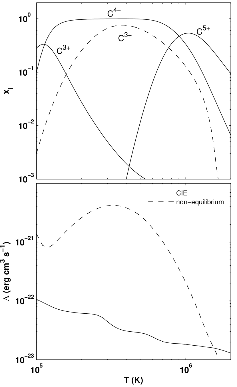
Figure 5.— Underionized gas in a model with $R=1.3$ kpc, $P_{\rm HIM}/k=50$ cm^-3 K, $T_{\rm HIM}=2\times 10^{6}$ K. (a) Non-equilibrium C³⁺ ion fraction (dashed curve). The carbon CIE ion fractions are shown by the solid curves for comparison. (b) Enhanced cooling in the underionized interface. The dashed curve shows the non-equilibrium cooling efficiency, and the solid curve shows the CIE cooling efficiency (for $Z=0.1$ solar).

We demonstrate the effect of “under-ionization” in Figure 5, for a model with $R=1.3$ kpc, $P_{\rm HIM}/k=50$ cm^-3 K, and $T_{\rm HIM}=2\times 10^{6}$ K ($\sigma_{0}=3.34$). In the upper panel we show the nonequilibrium C³⁺ ion fraction versus temperature (dashed curve), and the CIE ion fractions of C³⁺-C⁵⁺ (solid curves, Gnat & Sternberg 2007). The nonequilibrium C³⁺ abundance peaks at a temperature of $\sim 4\times 10^{5}$ K, whereas the CIE C³⁺ abundance peaks at $\sim 10^{5}$ K . For CIE, the dominant ion at $4\times 10^{5}$ K is C⁴⁺.

The modified ionization states enhance the cooling efficiency in this interface. We computed the local cooling efficiencies using Cloudy (version 07.02, Ferland et al. 1998) given our nonequilibrium ion fractions. This is shown in panel (b). The CIE cooling efficiency is shown by the solid curve (Gnat & Sternberg 2007). The non-equilibrium cooling efficiency (dashed curve) is an order of magnitude larger in this model, over a significant temperature range. This is mostly due to He⁺ which persists to much higher temperatures in the nonequilibrium gas compared to CIE.

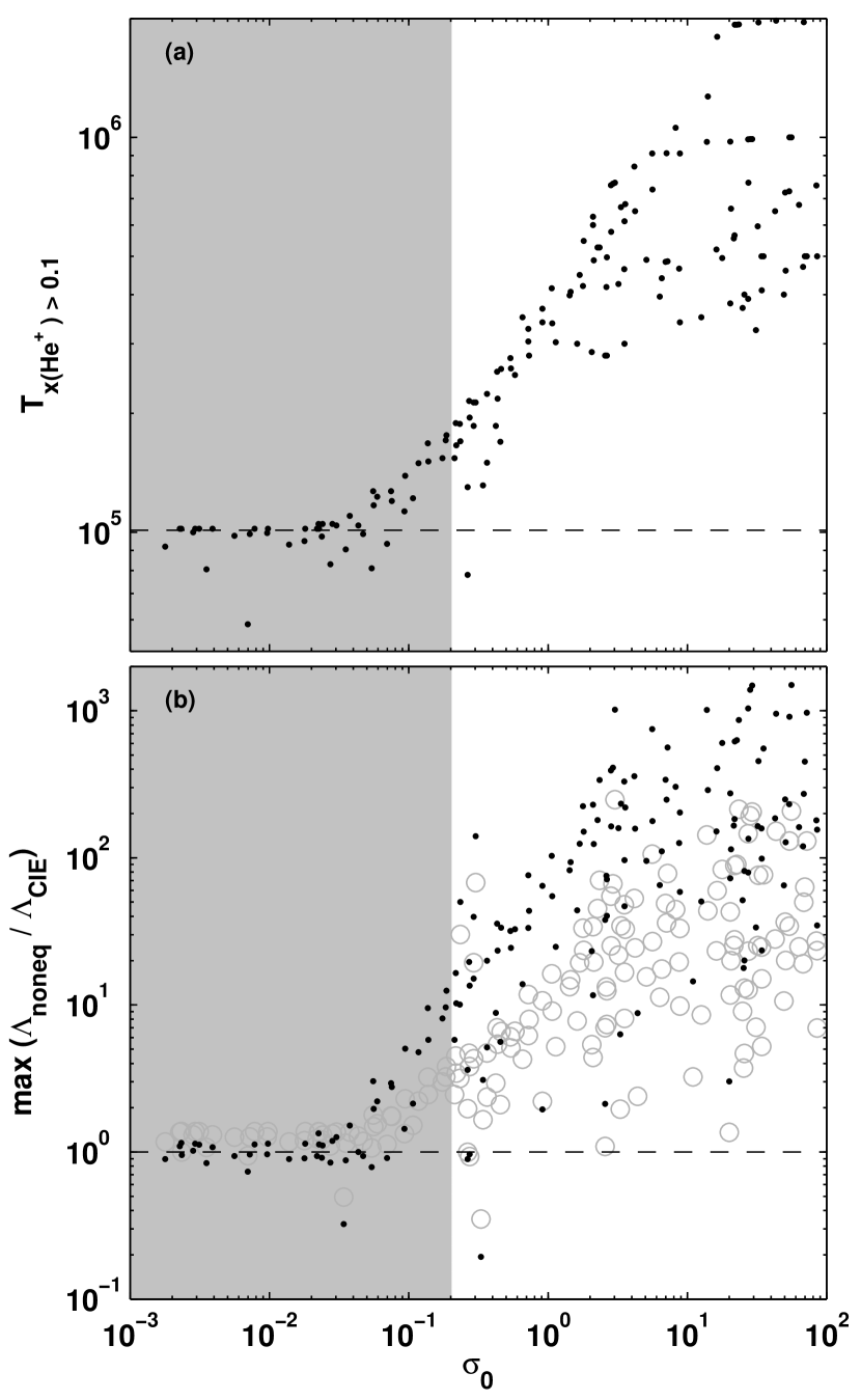
Figure 6.— Departures from equilibrium in conductive flows. (a) The temperature to which He⁺ persists, with a fractional abundance larger than $10\%$, in the non-equilibrium gas. The CIE value is shown by the dashed line. These results are independent of $Z$. (b) Maximal ratio of non-equilibrium to equilibrium cooling versus saturation for $Z=0.1$ solar (black points), and for $Z=1$ solar (gray circles). Models inside the shaded areas are not self-consistent, as cooling may not be neglected (see section 2.1.2).

In Figure 6 we demonstrate the effect of non-equilibrium ionization for our complete set of models. In panel (a) we show the ionization lag for He⁺. For each model, we plot the temperature to which He⁺ persists, with a fractional abundance larger than $10\%$, versus its saturation parameter. These values are independent of the gas metallicity. The corresponding CIE value ($\sim 10^{5}$ K) is shown by the dashed line. The shaded region indicates the range of saturation parameters for which no self-consistent evaporating solution exists (for $Z=0.1$ solar). In this region, radiative cooling may not be neglected (see section 2.1.2), and results in condensation. For the evaporating models, departures from equilibrium ionization can clearly be seen. He⁺ persists to higher temperatures than in CIE, despite the contribution of external photoionization by the metagalactic radiation field. For highly saturated models, in which the temperature profile is extremely steep, He⁺ may persist to $T\sim 10^{6}$ K.

The impact of these extended ion distributions on the cooling efficiencies is shown in panel (b). For each model we plot the maximal ratio of the non-equilibrium- to CIE-cooling efficiencies through the interface. The black points are for $Z=0.1$ times solar, and the gray circles are for $Z=1$. For the evaporating models, cooling is indeed enhanced by factors $\sim 5$ to $10^{3}$ relative to the CIE cooling efficiency.

These enhanced cooling efficiencies explain the results presented in section 2.1.2 (Figure 2). We found that for solar and $0.1$ solar metallicity gas, radiative cooling has a small impact on the dynamics of the flow for saturation parameters $\sigma_{0}>0.5$ and $\sigma_{0}>0.2$, respectively. Our results indicate that non-equilibrium effects significantly increase the value of $\sigma_{0}$ at which radiative effects set in. For comparison, in CIE radiative losses in solar metallicity gas become significant for $\sigma_{0}<0.1$ (for $\phi_{s}=0.3$, McKee and Cowie 1977), a factor of $\sim 5$ lower than for nonequilibrium cooling. The reason for this is that the cooling efficiencies in the underionized gas are larger, due to the enhanced contributions of He⁺ and metal-ion resonance-line cooling.

Does non-equilibrium ionization modify the observational signatures of evaporating clouds? In Figure 7(a) we compare the equilibrium (dashed curves) and non-equilibrium (solid curves) ion distributions versus position in the evaporating layers, for a model with $R=1.3$ kpc, $P_{\rm HIM}/k=50$ cm^-3 K, and $T_{\rm HIM}=2\times 10^{6}$ K. We show the abundances of C³⁺, N⁴⁺, O⁵⁺, and Si³⁺ including the effect of photoionization. The difference between the equilibrium and non-equilibrium curves is apparent: the non-equilibrium abundances reach their peaks further away from the cloud center (at higher temperatures) as the gas remains underionized, and they span considerably larger path-lengths than the equilibrium abundances. These larger path lengths result in enhanced column densities.

Finally, in panel (b) of Figure 7 we demonstrate the impact of photoionization by the metagalactic radiation field on the ionization states. Here we show a low-pressure model with $P_{\rm HIM}/k=0.1$ cm^-3 K, $T_{\rm HIM}=2\times 10^{6}$ K, and $R=7.5$ kpc. We compare the ionization state including photoionization by the metagalactic radiation field to the ionization in the absence of any external radiation. The presence of the external field increases the level of ionization both in the interface and in the surrounding HIM.

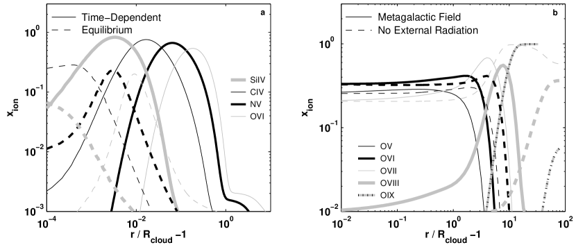
Figure 7.— (a) Non-equilibrium ionization in a high-pressure model with $R=1.3$ kpc, $P_{\rm HIM}/k=50$ cm^-3 K, and $T_{\rm HIM}=2\times 10^{6}$ K. The solid and dashed lines show the non-equilibrium and equilibrium abundances, respectively. The non-equilibrium abundances reach their peaks further away from the cloud center and span larger path-lengths. (b) The effect of photoionization by an external radiation field, for low-pressure model with $R=7.5$ kpc, $P_{\rm HIM}/k=0.1$ cm^-3 K, and $T_{\rm HIM}=2\times 10^{6}$ K. The solid and dashed lines show the abundances including photoionization by the metagalactic radiation file, and in the absence of external radiation, respectively. Photoionization increases the level of ionization in the interface.

Table 3Model Parameters

$T_{\rm HIM}$	$R$	$P/k_{\rm B}$	$U^{\ast}$		$\dot{m}_{\rm cl}$			$m_{7}/\dot{m}^{\ddagger}$
(K)	(kpc)	(cm-3 K)		$\sigma_{0}$	(g s-1)	$\omega$	max($M$)†	Gyr
$10^{6}$	$3$	$0.1$	$9.7\times 10^{-2}$	$85.62$	$6.45\times 10^{22}$	$0.03$	$0.60$	$330$
$10^{6}$	$3$	$1$	$9.7\times 10^{-3}$	$8.83$	$6.64\times 10^{22}$	$0.20$	$0.58$	$47.8$
$10^{6}$	$3$	$5$	$1.9\times 10^{-3}$	$1.81$	$6.80\times 10^{22}$	$0.63$	$0.38$	$14.8$
$10^{6}$	$3$	$10$	$9.7\times 10^{-4}$	$0.91$	$6.86\times 10^{22}$	$0.80$	$0.23$	$11.6$
$10^{6}$	$3$	$20$	$4.8\times 10^{-4}$	$0.46$	$6.93\times 10^{22}$	$0.89$	$0.13$	$10.3$
$10^{6}$	$3$	$50$	$1.9\times 10^{-4}$	$0.19$	$7.02\times 10^{22}$	$0.96$	$0.06$	$9.4$
${\bf 2\times 10^{6}}$	${\bf 1.3}$	${\bf 50}$	$1.9\times 10^{-4}$	${\bf 3.34}$	${\bf 1.67\times 10^{23}}$	${\bf 0.43}$	${\bf 0.50}$	${\bf 8.8}$
$2\times 10^{6}$	$3$	$0.1$	$9.7\times 10^{-2}$	$666.8$	$3.56\times 10^{23}$	$0.01$	$0.60$	$178$
$2\times 10^{6}$	$3$	$1$	$9.7\times 10^{-3}$	$68.70$	$3.66\times 10^{23}$	$0.04$	$0.60$	$43.4$
$2\times 10^{6}$	$3$	$5$	$1.9\times 10^{-3}$	$14.04$	$3.74\times 10^{23}$	$0.13$	$0.59$	$13.1$
$2\times 10^{6}$	$3$	$10$	$9.7\times 10^{-4}$	$7.08$	$3.77\times 10^{23}$	$0.24$	$0.57$	$7.0$
$2\times 10^{6}$	$3$	$20$	$4.8\times 10^{-4}$	$3.58$	$3.81\times 10^{23}$	$0.41$	$0.51$	$4.1$
$2\times 10^{6}$	$3$	$50$	$1.9\times 10^{-4}$	$1.45$	$3.86\times 10^{23}$	$0.69$	$0.33$	$2.4$
${\bf 2\times 10^{6}}$	${\bf 4.2}$	${\bf 1}$	$9.7\times 10^{-3}$	${\bf 49.40}$	${\bf 5.09\times 10^{23}}$	${\bf 0.05}$	${\bf 0.60}$	${\bf 24.9}$
$2\times 10^{6}$	$7.5$	$0.1$	$9.7\times 10^{-2}$	$266.7$	$8.87\times 10^{23}$	$0.01$	$0.60$	$71.6$
$2\times 10^{6}$	$7.5$	$1$	$9.7\times 10^{-3}$	$27.48$	$9.14\times 10^{23}$	$0.08$	$0.60$	$8.7$
$2\times 10^{6}$	$7.5$	$5$	$1.9\times 10^{-3}$	$5.62$	$9.34\times 10^{23}$	$0.29$	$0.56$	$2.3$
$2\times 10^{6}$	$7.5$	$10$	$9.7\times 10^{-4}$	$2.83$	$9.43\times 10^{23}$	$0.49$	$0.47$	$1.4$
$2\times 10^{6}$	$7.5$	$20$	$4.8\times 10^{-4}$	$1.43$	$9.52\times 10^{23}$	$0.70$	$0.33$	$0.95$
$2\times 10^{6}$	$7.5$	$50$	$1.9\times 10^{-4}$	$0.58$	$9.64\times 10^{23}$	$0.87$	$0.16$	$0.77$
$10^{7}$	$3$	$10$	$9.7\times 10^{-4}$	$831.1$	$1.98\times 10^{25}$	$0.007$	$0.60$	$4.7$
$10^{7}$	$3$	$20$	$4.8\times 10^{-4}$	$419.3$	$2.00\times 10^{25}$	$0.008$	$0.60$	$4.0$
$10^{7}$	$3$	$50$	$1.9\times 10^{-4}$	$169.7$	$2.02\times 10^{25}$	$0.02$	$0.60$	$1.9$
$10^{7}$	$7.5$	$10$	$9.7\times 10^{-4}$	$332.4$	$4.95\times 10^{25}$	$0.01$	$0.60$	$1.3$
$10^{7}$	$7.5$	$20$	$4.8\times 10^{-4}$	$167.7$	$4.99\times 10^{25}$	$0.02$	$0.60$	$0.75$
$10^{7}$	$7.5$	$50$	$1.9\times 10^{-4}$	$67.9$	$5.05\times 10^{25}$	$0.04$	$0.60$	$0.35$

Note. —

Results are shown for $\phi_{s}=0.3$.

$\ast$ – The ionization parameter $U=9.7\times 10^{-3}~{}(P/k_{\rm B})^{-1}$.

$\dagger$ – The maximal Mach number in the interface, max$(M)$.

$\ddagger$ – The evaporation time, $t_{\rm evap}\equiv m_{7}/\dot{m}$ Gyr, where $m_{7}$ is the warm cloud gas mass in units of $10^{7}$ M_⊙, and $\dot{m}=\omega\dot{m_{\rm cl}}$.

The highlighted lines correspond to the models considered in sections 4.1 and 4.2 below.

3.1. Metal Ion Fractions in Dwarf-Galaxy-Scale Objects

We now focus on the ion fractions in conductive interfaces surrounding dwarf galaxy-scale halos for comparison with the observed metal-ion absorbers. As a guide to the physical properties of dwarf-scale halos, we rely on the results presented in GS04, where we considered median halos with a virial mass $\sim 2\times 10^{9}$ M_⊙. For the dwarf-scale halos, we assume ambient temperatures of $10^{6}$ K, $2\times 10^{6}$ K, and $10^{7}$ K, gas cloud radii of $3$ kpc, $4.2$, and $7.5$ kpc, and bounding pressures in the range $0.1-50$ cm^-3 K. For bounding pressures in this range, the hydrogen in the $10^{4}$ K photoionized clouds is fully ionized at the surface, and the ionization parameter may be written as $U=9.7\times 10^{-3}~{}(P/k_{\rm B})^{-1}$.

In Table 3 we list the input parameters for the dwarf-scale models that we consider. These include the ambient temperature $T_{\rm HIM}$, the cloud radius $R$, and the gas pressure $P/k_{\rm B}$. We also list in Table 3 the ionization parameter $U$, saturation parameter $\sigma_{0}$, the classical (diffusive) mass loss rate $\dot{m}_{\rm cl}$, the mass-loss suppression factor $\omega=\dot{m}/\dot{m}_{\rm cl}$, the maximal Mach number in the flow, max$(M)$, and the evaporation time scale, $t_{\rm evap}\equiv m_{7}/\dot{m}$, for clouds with warm gas masses of $10^{7}$ M_⊙. All the values listed in Table 3 are computed assuming $\phi_{s}=0.3$.

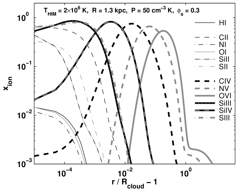
Figure 8.1.— Ion fractions as a function of scaled radius $r/R-1$, in conductive interfaces surrounding dwarf-galaxy-halos. The ambient temperature, $T_{\rm HIM}$, cloud radius, $R$, and bounding pressure, $P$ are indicated in each panel. In Fig 8.1 the non-equilibrium ion fractions are for $T_{\rm HIM}=2\times 10^{6}$ K, $R=1.3$ kpc, and $P/k_{\rm B}=50$ cm^-3 K.

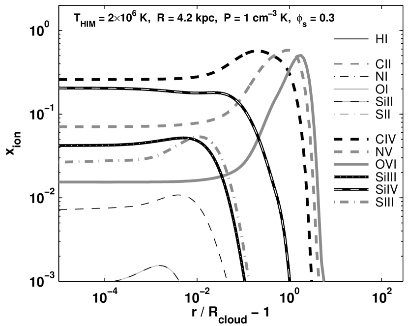
Figure 8.2.— Same as figure 8.1 but for $T_{\rm HIM}=2\times 10^{6}$ K, $R=4.2$ kpc, and $P/k_{\rm B}=1$ cm^-3 K.

In Figure set 8, we present the ion fractions as a function of distance from the cloud surface for the grid of dwarf galaxy-scale models. The ambient temperature, $T_{\rm HIM}$, cloud radius, $R$, and bounding pressure, $P/k_{\rm B}$ are indicated in each panel. Figure 8 displays the ion fractions of the low ions C II, N I, O I, Si II, and S II, and the high-ions C IV, N V, O VI, Si III, Si IV, and S III. These are the ions that were measured by Sembach et al. (1999, 2000), Collins et al. (2004), and Fox et al. (2005) in the high-velocity metal ion absorbers (see e.g. Table 1).

4. Metal-Absorption Column Densities

In this section we present computations of the integrated metal-ion column densities that are produced in the conductively evaporating layers.

The characteristic column density in an interface, $N_{\rm HIM}\equiv n_{\rm HIM}R$, is given by (see equation 5),

$$N_{\rm HIM}=2\times\frac{2\kappa_{\rm HIM}T_{\rm HIM}}{25\phi_{s}\mu_{\rm HIM}c^{3}_{\rm HIM}}=1.7\times 10^{17}\;\frac{T_{6,{\rm HIM}}^{2}}{\sigma_{0}\phi_{0.3}}\;\;{\rm cm}^{-2},$$ (19)

where $\mu_{\rm HIM}$ is the mean mass per particle, $T_{6,{\rm HIM}}$ is the HIM temperature in units of $10^{6}$ K, and $\phi_{0.3}=\phi_{\rm s}/0.3$. This equation shows that in general, models with lower saturation parameters produce larger columns. The column density of a given ionic species is related to this characteristic column by an “ionization correction”, that depends on the interface parameters.

For gas in collisional ionization equilibrium, the local ion fractions are a function of the temperature only. The ionization correction and implied metal-ion column densities therefore depend only on $\sigma_{0}$ (through its control of the temperature profile, see Figure 1) and on the ambient temperature, $T_{\rm HIM}$. However, the functional dependence on $\sigma_{0}$ and $T_{\rm HIM}$ may be complicated.

For non-equilibrium conditions, departures from equilibrium ionization and the ion fractions at a given temperature depend on the ratio of the heating time-scale and the ionization time-scale. Equation 17 shows that in the absence of photoionization, the non-equilibrium abundances and columns still depend only on $\sigma_{0}$ and $T_{\rm HIM}$. The inclusion of photoionization by the metagalactic radiation field introduces an implicit dependence on the gas density (or ionization parameter, see equation 18). The non-equilibrium column densities are therefore general functions of all three interface parameters.

Here we wish to find conditions that yield metal-ion column densities comparable to those observed in the high-velocity ionized absorbers, including the high observed O VI column ($N_{\rm O\,VI}\sim 10^{14}$ cm^-2). We focus on the column densities of the high ions C IV, N V, O VI, Si III, Si IV, and S III, as a function of the impact parameter from the cloud center, $b$. In Table 4, we list the (two-sided) central ($b=0$) and maximal column densities for the different models considered in section 3. For the evaporating gas, the line-of-sight column density of ion $i$ of element $m$ observed at an impact parameter $b$ is,

$$N_{i}=2\int_{{\rm max}(b,R)}^{\infty}\frac{n_{\rm H}(r)A_{m}x_{i}(r)rdr}{\sqrt{r^{2}-b^{2}}},$$ (20)

where $A_{m}$ is the abundance of element $m$ relative to hydrogen, $n_{\rm H}(r)$ is the position dependent hydrogen density, and $x_{i}(r)$ are the position-dependent ion fractions, as presented in section 3. The maximal columns are evaluated for each ion independently, and occur at different impact parameters for each ion and model.

The results presented in Table 4 are computed for $Z=0.1$ times solar. Since the fractional ion abundances are independent of metallicity, the integrated columns are proportional to $Z$. (However, as discussed in 2.1.2, the range of $\sigma_{0}$ values for which a self-consistent evaporating solution can be found is a function of $Z$.)

Table 4 lists the central column densities produced in the interface layers. When observing evaporating clouds, the observed absorption line properties will generally depend not only on the conductive interface, but also on the ionization properties of the embedded photoionized clouds. In the text that follows we discuss, as illustrative examples, the total (cloud $+$ interface) column densities that arise in two specific models. First we consider a low-ionization cloud embedded in a high-pressure corona, with $P/k_{\rm B}=50$ cm^-3 K (§4.1), and then we study a more highly-ionized cloud embedded a low-pressure medium, with $P/k_{\rm B}=1$ cm^-3 K (in §4.2). The lines representing these two illustrative models are highlighted in Table 3.

4.1. A Low-Ionization Cloud Embedded in a High Pressure Medium

As an example for a low-ionization photoionized cloud embedded in a high-pressure corona, we rely on the physical properties of the “CHVC-scale” model presented in GS04 (“model A” in GS04). This model represents a $10^{8}$ M_⊙ dark-matter halo that contains a warm gas mass of $1.1\times 10^{6}$ M_⊙, which is subjected to an external bounding pressure, $P/k_{\rm B}=50$ cm^-3 K. The resulting photoionized cloud has a radius $R=1.3$ kpc. The ionization parameter on the cloud surface is low, $U=1.9\times 10^{-4}$, and high ions are thus inefficiently produces in this cloud. Here we assume that the cloud is surrounded by a hot Galactic corona, with a temperature $T_{\rm HIM}=2\times 10^{6}$ K, and photoionized by the metagalactic radiation field.

These parameters imply that the cloud evaporates in a marginally-saturated flow, with $\sigma_{0}\simeq 3.3$. The mass loss rate is suppressed by a factor $0.43$ relative to that in a classical diffusive flow, and the maximal Mach number in the flow is $0.50$.

Figure 8.1 displays the ion fractions that arise in the conductive interface in this model. In evaluating the absorption-line signatures that arise from the evaporating cloud, we use the abundances given in GS04 for “model A” (Figure 3 in GS04) for the ion fractions within the photoionized cloud, and the ion fractions computed here and presented in Figure 8.1 for the evaporating layers. We then evaluate the projected column densities as a function of impact parameter from the cloud center. These column densities include the contributions of both the photoionized cloud and the conductive interface surrounding it.

Figure 9 shows the projected column densities in our evaporating high-pressure model. The ionization in this conductive interface results in a maximal O VI column density of $3.2\times 10^{12}$ cm^-2 (compared to $4.5\times 10^{6}$ cm^-2 in the purely photoionized cloud), and a C IV column density of $2.5\times 10^{12}$ cm^-2 (compared to $2.6\times 10^{11}$ cm^-2 in the purely photoionized cloud). The evaporating layers increase the O VI column by $\sim 6$ orders of magnitude, and the C IV column by $\sim 1$ order of magnitude relative to the purely photoionized cloud discussed in GS04. However, for this model, the enhanced columns still do not bring the model into harmony with the observations of the high-velocity metal-ion absorbers (see e.g. Table 1).

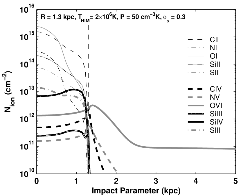
Figure 9.— Projected column densities as a function of impact parameter in a high-pressure model. For this model $R=1.3$ kpc, $P/k_{\rm B}=50$ cm^-3 K, and $T_{\rm HIM}=2\times 10^{6}$ K.

For pressure supported photoionized clouds in high-pressure environments ($P\sim 50$ cm${}^{-3}~{}K$), the ionization parameter is generally too low to allow for efficient production of high ions such as C³⁺ and O⁵⁺. The high-ion column densities are therefore dominated by ions produced in the evaporating layers, and are not significantly affected by the details of the cloud’s ionization state.

4.2. A Highly-ionized Cloud Embedded in a Low Pressure Medium

As an illustrative example for the physical properties of a more highly ionized photoionized cloud embedded in a low-pressure medium, we rely on the standard dwarf-scale model presented in GS04 (“model C” in GS04), based on the observed properties of Local Group dwarf galaxies Leo A and Sag DIG (Sternberg et al. 2002). This model represents a $2\times 10^{9}$ M_⊙ dark-matter halo that contains a total warm gas mass of $1.6\times 10^{7}$ M_⊙, and is subjected to an external bounding pressure $P/k_{\rm B}=1$ cm^-3 K. The resulting cloud has a radius $R\sim 4.2$ kpc. The ionization parameter on the surface of this cloud is higher, $U=9.7\times 10^{-3}$, and high ions such as C³⁺ and N⁴⁺ are efficiently produced in the ionized envelopes of this cloud. Here we assume that the halo is surrounded by a hot intergalactic medium, with a temperature $T_{\rm HIM}=2\times 10^{6}$ K, and is photoionized by the metagalactic radiation field.

Table 4Column Densities

THIM	R	P/kB	$\sigma_{0}$		C IV	N V	O VI	Si III	Si IV	S III
$10^{6}$	$3$	$0.1$	85.62	central	$8.9\times 10^{9}$	$7.1\times 10^{9}$	$8.6\times 10^{10}$	$0.0$	$9.0\times 10^{6}$	$1.9\times 10^{5}$
				maximal	$2.9\times 10^{10}$	$1.8\times 10^{10}$	$1.9\times 10^{11}$	$0.0$	$4.7\times 10^{7}$	$6.2\times 10^{5}$
$10^{6}$	$3$	$1$	8.83	central	$1.6\times 10^{11}$	$5.0\times 10^{10}$	$3.8\times 10^{11}$	$5.2\times 10^{8}$	$4.0\times 10^{9}$	$2.8\times 10^{8}$
				maximal	$4.8\times 10^{11}$	$7.8\times 10^{11}$	$5.6\times 10^{11}$	$6.3\times 10^{9}$	$2.9\times 10^{10}$	$2.8\times 10^{9}$
$10^{6}$	$3$	$5$	1.81	central	$3.6\times 10^{11}$	$1.3\times 10^{11}$	$1.1\times 10^{12}$	$5.4\times 10^{9}$	$2.0\times 10^{10}$	$2.1\times 10^{9}$
				maximal	$1.1\times 10^{12}$	$2.7\times 10^{11}$	$2.0\times 10^{12}$	$9.9\times 10^{10}$	$1.5\times 10^{11}$	$3.6\times 10^{10}$
$10^{6}$	$3$	$10$	0.91	central	$4.5\times 10^{11}$	$1.7\times 10^{11}$	$1.7\times 10^{12}$	$1.2\times 10^{10}$	$2.9\times 10^{10}$	$5.5\times 10^{9}$
				maximal	$2.1\times 10^{12}$	$4.9\times 10^{11}$	$3.5\times 10^{12}$	$2.9\times 10^{11}$	$2.6\times 10^{11}$	$1.3\times 10^{11}$
$10^{6}$	$3$	$20$	0.46	central	$5.4\times 10^{11}$	$2.2\times 10^{11}$	$2.5\times 10^{12}$	$1.3\times 10^{10}$	$3.6\times 10^{10}$	$6.9\times 10^{9}$
				maximal	$3.7\times 10^{12}$	$8.5\times 10^{11}$	$6.2\times 10^{12}$	$3.7\times 10^{11}$	$4.6\times 10^{11}$	$1.8\times 10^{11}$
$10^{6}$	$3$	$50$	0.19	central	$7.4\times 10^{11}$	$3.5\times 10^{11}$	$4.5\times 10^{12}$	$5.2\times 10^{10}$	$5.1\times 10^{10}$	$2.9\times 10^{10}$
				maximal	$7.0\times 10^{12}$	$1.6\times 10^{12}$	$1.2\times 10^{13}$	$1.8\times 10^{12}$	$8.8\times 10^{11}$	$9.3\times 10^{12}$
$2\times 10^{6}$	$1.3$	$50$	3.34	central	$4.2\times 10^{11}$	$1.6\times 10^{11}$	$1.3\times 10^{12}$	$7.6\times 10^{9}$	$2.5\times 10^{10}$	$3.6\times 10^{9}$
				maximal	$2.5\times 10^{12}$	$5.4\times 10^{11}$	$3.2\times 10^{12}$	$2.3\times 10^{11}$	$3.3\times 10^{11}$	$1.0\times 10^{11}$
$2\times 10^{6}$	$3$	$0.1$	666.8	central	$8.2\times 10^{9}$	$6.1\times 10^{9}$	$6.9\times 10^{10}$	$0.0$	$8.8\times 10^{6}$	$2.8\times 10^{5}$
				maximal	$3.1\times 10^{10}$	$1.9\times 10^{10}$	$1.8\times 10^{11}$	$0.0$	$5.1\times 10^{7}$	$1.5\times 10^{6}$
$2\times 10^{6}$	$3$	$1$	68.70	central	$1.5\times 10^{11}$	$3.6\times 10^{10}$	$2.3\times 10^{11}$	$4.5\times 10^{8}$	$3.8\times 10^{9}$	$2.1\times 10^{8}$
				maximal	$4.2\times 10^{11}$	$5.9\times 10^{10}$	$3.1\times 10^{11}$	$4.8\times 10^{9}$	$2.5\times 10^{10}$	$1.7\times 10^{9}$
$2\times 10^{6}$	$3$	$5$	14.04	central	$3.1\times 10^{11}$	$9.4\times 10^{10}$	$6.1\times 10^{11}$	$4.9\times 10^{9}$	$1.8\times 10^{10}$	$1.8\times 10^{9}$
				maximal	$9.4\times 10^{11}$	$1.7\times 10^{11}$	$9.5\times 10^{11}$	$9.3\times 10^{10}$	$1.4\times 10^{11}$	$3.3\times 10^{10}$
$2\times 10^{6}$	$3$	$10$	7.08	central	$3.7\times 10^{11}$	$1.2\times 10^{11}$	$9.0\times 10^{11}$	$6.3\times 10^{9}$	$2.2\times 10^{10}$	$2.8\times 10^{9}$
				maximal	$1.5\times 10^{12}$	$30.\times 10^{11}$	$1.6\times 10^{12}$	$1.5\times 10^{11}$	$2.0\times 10^{11}$	$6.6\times 10^{10}$
$2\times 10^{6}$	$3$	$20$	3.58	central	$4.1\times 10^{11}$	$1.5\times 10^{11}$	$1.3\times 10^{12}$	$1.7\times 10^{10}$	$2.6\times 10^{10}$	$8.0\times 10^{9}$
				maximal	$2.4\times 10^{12}$	$5.0\times 10^{11}$	$2.9\times 10^{12}$	$6.7\times 10^{11}$	$3.1\times 10^{11}$	$3.2\times 10^{11}$
$2\times 10^{6}$	$3$	$50$	1.45	central	$4.7\times 10^{11}$	$1.9\times 10^{11}$	$2.0\times 10^{12}$	$8.2\times 10^{9}$	$2.9\times 10^{10}$	$3.9\times 10^{9}$
				maximal	$4.7\times 10^{12}$	$1.1\times 10^{12}$	$6.8\times 10^{12}$	$3.6\times 10^{11}$	$6.0\times 10^{11}$	$1.6\times 10^{11}$
$2\times 10^{6}$	$4.2$	$1$	49.40	central	$1.7\times 10^{11}$	$4.5\times 10^{10}$	$2.8\times 10^{11}$	$5.1\times 10^{8}$	$4.2\times 10^{9}$	$2.4\times 10^{8}$
				maximal	$5.7\times 10^{11}$	$7.9\times 10^{10}$	$3.9\times 10^{11}$	$6.8\times 10^{9}$	$3.5\times 10^{10}$	$2.4\times 10^{9}$
$2\times 10^{6}$	$7.5$	$0.1$	226.7	central	$1.2\times 10^{10}$	$9.7\times 10^{9}$	$1.1\times 10^{11}$	$0.0$	$1.0\times 10^{7}$	$0.0$
				maximal	$5.2\times 10^{10}$	$3.3\times 10^{10}$	$3.2\times 10^{11}$	$0.0$	$7.9\times 10^{7}$	$0.0$
$2\times 10^{6}$	$7.5$	$1$	27.48	central	$2.1\times 10^{11}$	$6.2\times 10^{10}$	$4.0\times 10^{11}$	$6.3\times 10^{8}$	$4.4\times 10^{9}$	$3.7\times 10^{8}$
				maximal	$8.4\times 10^{12}$	$1.2\times 10^{11}$	$5.6\times 10^{11}$	$1.1\times 10^{10}$	$4.7\times 10^{10}$	$5.5\times 10^{9}$
$2\times 10^{6}$	$7.5$	$5$	5.62	central	$3.4\times 10^{11}$	$1.3\times 10^{11}$	$9.9\times 10^{12}$	$8.1\times 10^{9}$	$2.1\times 10^{10}$	$4.0\times 10^{9}$
				maximal	$1.7\times 10^{12}$	$3.5\times 10^{11}$	$1.9\times 10^{12}$	$3.0\times 10^{11}$	$2.7\times 10^{11}$	$1.4\times 10^{11}$
$2\times 10^{6}$	$7.5$	$10$	2.83	central	$4.1\times 10^{11}$	$1.6\times 10^{11}$	$1.4\times 10^{12}$	$4.3\times 10^{9}$	$2.2\times 10^{10}$	$1.9\times 10^{9}$
				maximal	$2.8\times 10^{12}$	$6.0\times 10^{11}$	$3.6\times 10^{12}$	$1.7\times 10^{11}$	$3.3\times 10^{11}$	$7.1\times 10^{10}$
$2\times 10^{6}$	$7.5$	$20$	1.43	central	$4.7\times 10^{11}$	$1.9\times 10^{11}$	$1.9\times 10^{12}$	$2.0\times 10^{10}$	$3.1\times 10^{10}$	$9.7\times 10^{0}$
				maximal	$4.7\times 10^{12}$	$1.1\times 10^{12}$	$6.7\times 10^{12}$	$1.2\times 10^{12}$	$6.1\times 10^{11}$	$5.6\times 10^{11}$
$2\times 10^{6}$	$7.5$	$50$	0.58	central	$5.7\times 10^{11}$	$2.4\times 10^{11}$	$2.9\times 10^{12}$	$3.5\times 10^{10}$	$4.2\times 10^{10}$	$1.7\times 10^{10}$
				maximal	$9.6\times 10^{12}$	$2.1\times 10^{12}$	$1.4\times 10^{13}$	$2.3\times 10^{12}$	$1.3\times 10^{12}$	$1.1\times 10^{12}$
$10^{7}$	$3$	$10$	831.1	central	$3.9\times 10^{11}$	$1.3\times 10^{11}$	$9.6\times 10^{11}$	$1.1\times 10^{10}$	$2.2\times 10^{10}$	$4.7\times 10^{09}$
				maximal	$1.7\times 10^{12}$	$3.4\times 10^{11}$	$1.7\times 10^{12}$	$3.4\times 10^{11}$	$2.1\times 10^{11}$	$1.4\times 10^{11}$
$10^{7}$	$3$	$20$	419.3	central	$4.1\times 10^{11}$	$1.5\times 10^{11}$	$1.2\times 10^{12}$	$1.2\times 10^{10}$	$2.5\times 10^{10}$	$6.0\times 10^{09}$
				maximal	$2.4\times 10^{12}$	$4.8\times 10^{11}$	$2.6\times 10^{12}$	$6.1\times 10^{11}$	$3.1\times 10^{11}$	$3.0\times 10^{11}$
$10^{7}$	$3$	$50$	169.7	central	$4.4\times 10^{11}$	$1.7\times 10^{11}$	$1.5\times 10^{12}$	$7.6\times 10^{09}$	$2.6\times 10^{10}$	$3.4\times 10^{09}$
				maximal	$4.1\times 10^{12}$	$8.7\times 10^{11}$	$5.0\times 10^{12}$	$3.2\times 10^{11}$	$5.2\times 10^{11}$	$1.4\times 10^{11}$
$10^{7}$	$7.5$	$10$	332.4	central	$4.2\times 10^{11}$	$1.5\times 10^{11}$	$1.3\times 10^{12}$	$1.2\times 10^{10}$	$2.4\times 10^{10}$	$5.4\times 10^{09}$
				maximal	$2.7\times 10^{12}$	$5.5\times 10^{11}$	$3.0\times 10^{12}$	$5.1\times 10^{11}$	$3.4\times 10^{11}$	$2.3\times 10^{11}$
$10^{7}$	$7.5$	$20$	167.7	central	$4.4\times 10^{11}$	$1.7\times 10^{11}$	$1.5\times 10^{12}$	$1.6\times 10^{10}$	$2.7\times 10^{10}$	$7.1\times 10^{09}$
				maximal	$4.1\times 10^{12}$	$8.7\times 10^{11}$	$5.0\times 10^{12}$	$8.9\times 10^{11}$	$5.3\times 10^{11}$	$3.9\times 10^{11}$
$10^{7}$	$7.5$	$50$	67.88	central	$4.6\times 10^{11}$	$1.8\times 10^{11}$	$1.7\times 10^{12}$	$2.3\times 10^{10}$	$3.0\times 10^{10}$	$9.5\times 10^{09}$
				maximal	$7.0\times 10^{12}$	$1.5\times 10^{12}$	$9.0\times 10^{12}$	$1.7\times 10^{12}$	$9.3\times 10^{11}$	$6.7\times 10^{11}$

Note. — Assuming $\phi_{s}=0.3$. Columns were computed for $Z=0.1$ times solar, and are proportional to $Z$.

This cloud then evaporates in a saturated flow, with $\sigma_{0}\sim 50$. The mass-loss rate is suppressed by a factor $0.05$ relative to a classical diffusive flow, and the maximal Mach number in the flow is $0.60$.

Figure 8.2 displays the ion fractions of the low ions C II, N I, O I, Si II, and S II, and the high-ions C IV, N V, O VI, Si III, Si IV, and S III in the conductive interface surrounding this dwarf scale halo.

For the column densities produced in this model, we rely on the ion-abundances given in GS04 (“model C”, Figure 5) for the photoionized component, and the ion fractions computed here and presented in Figure 8.2 for the conductive interface surrounding it. We compute the projected column densities as a function of impact parameter from the cloud center, again including both the photoionized core and the surrounding evaporating envelope.

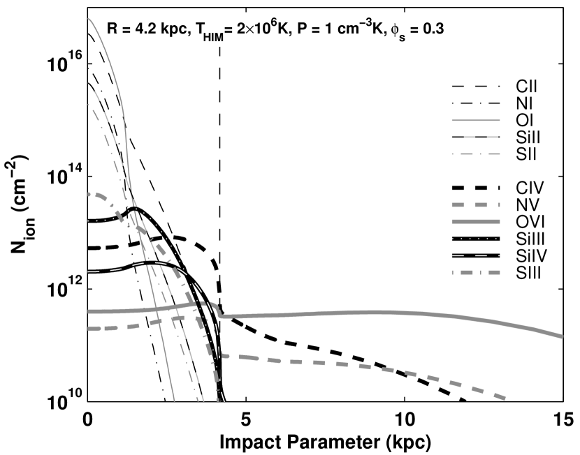
Figure 10.— Projected column densities as a function of impact parameter in a dwarf galaxy-scale model. For this model $R=4.2$ kpc, $P/k_{\rm B}=1$ cm^-3 K, and $T_{\rm HIM}=2\times 10^{6}$ K.

Figure 10 shows the projected column densities in our dwarf-galaxy-scale model. The ionization in this conductive interface results in a maximal O VI column density of $5.5\times 10^{11}$ cm^-2 (compared to $2.9\times 10^{11}$ cm^-2 in the photoionized cloud), and a maximal C IV column density of $8.3\times 10^{12}$ cm^-2, comparable to that produced in the photoionized cloud). This is only a minor enhancement relative to the purely photoionized cloud, and the columns in this dwarf galaxy-scale model are therefore still too low to account for the observed properties of the metal-ion absorbers (e.g. Table 1).

4.3. Diagnostics

Diagnostic diagrams for evaporating gas may be constructed using Equation 20 and the computational data presented in § 3, and used to probe the ionization mechanisms at play in observed metal-ion absorbers. As an example,

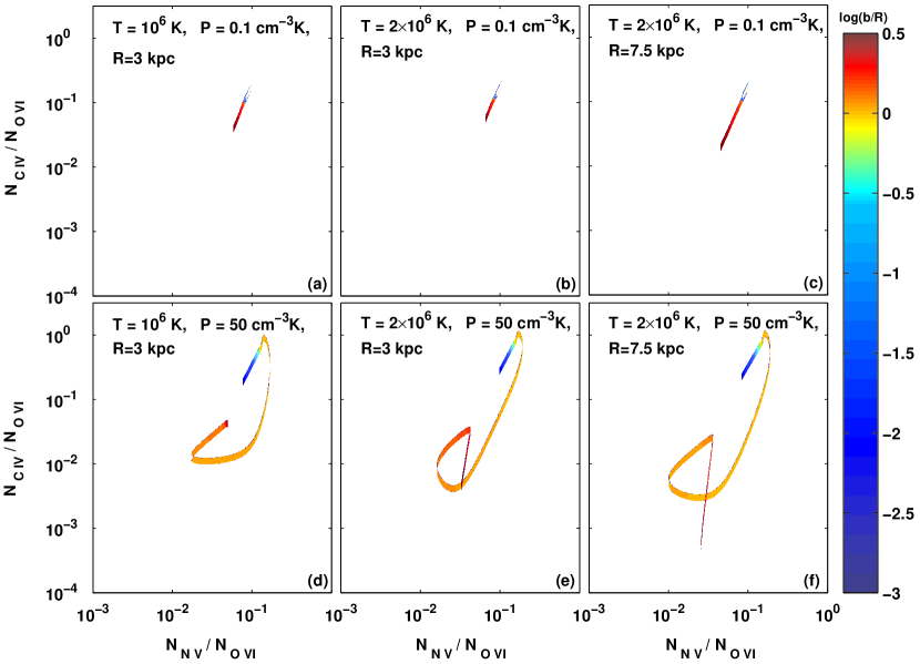
Figure 11.— Column density ratios $N_{\rm C~{}IV}/N_{\rm O~{}VI}$ versus $N_{\rm N~{}V}/N_{\rm O~{}VI}$ for evaporating gas. The impact parameter $b$ is indicated by the color along the trajectories, from the cloud center (blue) to the surrounding HIM (red). The different panels are for different interface parameters, as indicated by the legends. These ion ratios do not include any contribution from the embedded warm cloud.

in Figure  11 we display trajectories for $N_{\rm C~{}IV}/N_{\rm O~{}VI}$ versus $N_{\rm N~{}V}/N_{\rm O~{}VI}$, as a function of impact parameter, $b$ through the evaporative interface. The impact parameter is represented by the color along the curves, from the cloud center where $b=0$ (blue) to the surrounding HIM where $b>R$ (red). The different panels are for non-equilibrium evaporation for a range of dwarf-scale objects, drawn from the range of cloud radii, bounding pressures, and HIM temperatures considered in Table 4. These diagrams show the possible range of ion ratios produced in evaporating dwarf-scale models. Since the column densities are proportional to the metallicity, the ion ratios are independent of $Z$. Note that these ion ratios do not include any contribution from the embedded warm cloud, which depends on the astrophysical setting.

O⁵⁺ is the most highly ionized of the three ions that we consider. $N_{\rm C~{}IV}/N_{\rm O~{}VI}$ and $N_{\rm N~{}V}/N_{\rm O~{}VI}$ are therefore large at low temperatures where the O⁵⁺ fraction is small, and decrease at higher temperature as O⁵⁺ becomes more abundant. Small impact parameters (in blue) sample the lower-$T$ parts of the interface, where $N_{\rm C~{}IV}/N_{\rm O~{}VI}$ and $N_{\rm N~{}V}/N_{\rm O~{}VI}$ are large. The cooling trajectories therefore start in the upper right corner of the parameter space. Larger impact parameters only sample the hotter parts of the interface, and the trajectories evolve in the direction of decreasing $N_{\rm C~{}IV}/N_{\rm O~{}VI}$ and $N_{\rm N~{}V}/N_{\rm O~{}VI}$. Finally, as the temperature approaches $T_{\rm HIM}$ ($2\times 10^{6}$ K in Figure 11), O⁵⁺ is replaced by higher ionization states, and the evolutionary tracks turn up again.

An additional ion that is commonly observed in high-velocity absorbers, and that has been used as a diagnostic for the physical conditions prevailing in these systems, is Si III (Collins et al. 2004; Collins et al. 2009; Shull et al. 2009). The typical observed column densities of Si III in the high-velocity absorbers are $\sim 3\times 10^{13}$ cm^-2 (Shull et al. 2009). Si III is never efficiently produced in evaporating dwarf-galaxy-scale clouds. For low bounding pressures the ionization parameter is too high to efficiently produce Si III in the evaporating layers, but even at high pressures ($P\sim 50$ cm^-3 K), for which Si III is the dominant ionization state at the cloud surface, columns in excess of $10^{12}$ cm^-2 are rarely produced. Si III must therefore be produced by alternative ionization mechanisms. It may be efficiently produced by photoionization within an embedded warm cloud, as we demonstrate in Figures 9 and 10.

4.4. High O VI columns in evaporating clouds?

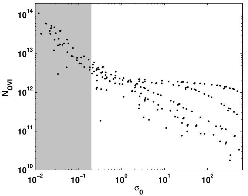
Figure 12.— Central (two-sided) O VI column density versus saturation. Models inside the shaded areas are not self-consistent, as cooling may not be neglected (see section 2.1.2).

The results presented in Table 4 and illustrated by the examples discussed above, show that the typical O VI columns that are produced in the different dwarf-scale models are $\leq 10^{13}$ cm^-2. Can column densities of order $10^{14}$ cm^-2 be produced in conductively evaporating clouds?

In Figure 12 we show the central (two-sided) O VI column density as a function of saturation parameter for our full grid of models, assuming $Z=0.1$. The range of saturation parameters for which no self-consistent evaporating solution can be found has been shaded in the plot. In the shaded region, cooling overcomes conductive heating, evaporation stops, and instead the ambient medium condenses onto the clouds. Our theory does not apply to condensing clouds. Figure 12 shows that central O VI column densities of order $10^{14}$ cm^-2 cannot be obtained for any $Z=0.1$ evaporating model. The largest central O VI columns, obtained for $\sigma_{0}\sim 0.2$, are $\sim 2\times 10^{12}$ cm^-2.

We note that for solar metallicity clouds, the O VI columns are a factor of $10$ larger. However, since for $Z=1$ self-consistent evaporating solutions can only be found for $\sigma_{0}>0.5$, central O VI columns of order $10^{14}$ cm^-2 can still not be obtained.

Since the observed column density is a function of the impact parameter, we also computed the maximal O VI column density obtained in each self-consistent evaporating model. Inspecting our entire parameter space ($0.1<P/k_{\rm B}<10^{4}$ cm^-3 K, $1$ pc $<R<100$ kpc, $5\times 10^{5}<T<10^{7}$ K), we find that for $Z=0.1$, maximal column densities of order $10^{14}$ cm^-2 only occur in evaporating clouds ($\sigma_{0}>0.2$) for extreme combinations of parameters, with $T\sim 10^{7}$ K, and $P\sim 10^{4}$ cm^-3 K. We therefore conclude that non-equilibrium ionization in conductively evaporating clouds an unlikely explanation of the high-ions observed in the high-velocity metal-ion absorbers. An alternative explanation is that O VI is created in a flow of cooling gas (e.g. Edgar & Chevalier 1986; Heckman et al. 2002; Gnat & Sternberg 2007; Gnat & Sternberg 2009).

While a conductive origin for the O VI absorption observed in the ionized high-velocity clouds appears unlikely, recent observations indicate that evaporating O VI may be present in more local environments. Savage & Lehner (2006) report on FUSE absorption line observations toward a sample of local white dwarfs. O VI was detected along 24 lines of sight, with column densities between $2.5\times 10^{12}$ and $4.0\times 10^{13}$ cm^-2. Based on the observed columns and on the kinematics of the absorption, Savage & Lehner suggest that this sample of local absorbers may probe conductive interfaces in the local interstellar medium. Their analysis relied on the plane-parallel conduction-front models of Borkowski et al. (1990). Our spherical models for typical interstellar parameters ($T\sim 10^{6}$ K, $P\sim 4\times 10^{3}$ cm^-3 K, and $R\sim 15$ pc) support this interpretation. For interstellar conditions the saturation parameter $\sigma_{0}\sim 0.5$, and we find that O VI column densities of order $10^{13}$ cm^-2 are expected for solar metallicity gas. The predicted Doppler widths ($15-30$ km s^-1) and flow velocities ($5-55$ km s^-1) are also consistent with the Savage & Lehner observations.

5. Summary

In this paper we present computations of the non-equilibrium ionization states of H, He, C, N, O, Si, and S in thermally conductive interfaces, surrounding warm (and photoionized) gas clouds that undergo steady evaporation into a hot ambient medium.

We rely on the formalism developed by Dalton & Balbus (1993; DB93) for solving the temperature profile in the evaporating gas. This formalism allows the thermal conductivity to change continuously from the classical diffusive form (Spitzer 1962) to a flux-limited saturated form (Cowie & McKee 1977). The temperature profile then depends only on the global level of saturation in the flow, as described by the saturation parameter, $\sigma_{0}$.

In their analytic solution for the temperature profile, DB93 neglect the kinetic energy term as well as the radiative losses term in the energy equation. As opposed to previous claims, we find that the neglect of the kinetic energy term is accurate only for classical, unsaturated flows, and applies to saturated flows only if the parameter $\phi_{s}$ (see Equation 2) is less than $0.6$.

We explicitly solve the time-dependent ionization equations for the evaporating gas, including also photoionization by the present-day metagalactic field. As the gas evaporates, heating can become fast compared to the ionization time-scale, and the gas tends to remain under-ionized. We study how departures from equilibrium ionization affects the ion distributions and resulting cooling rates in the evaporating layers. We show that the existence of underionized species, most significantly He⁺, significantly enhances the cooling rates. We estimate numerically the range of saturation parameters for which radiative cooling plays a significant role in determining the dynamics of the gas. We find that for a $0.1$ ($1$) times solar metallicity gas, radiative losses are significant for $\sigma_{0}\lesssim 0.2$ ($0.5$). For larger values of $\sigma_{0}$ the importance of radiative cooling is generally smaller, and depends on the neutral fraction at the surface of the evaporating cloud.

We use our conduction models to extend the purely photoionized cloud models for local high-velocity metal line absorbers that we presented in Gnat & Sternberg (2004; GS04). In that paper, we modeled the absorbers as warm ($\sim 10^{4}$ K) clouds that are photoionized by the metagalactic radiation field, and embedded in low-mass ($<2\times 10^{9}$ M_⊙) dark-matter mini-haos. Here, we consider the additional ionization that occurs in the conductive envelopes, as these clouds evaporate into a hot corona and/or intergalactic medium. We consider a wide range of input parameters (cloud radius, thermal pressure and temperature of the hot medium) as summarized in Table 3. This table also lists the ionization parameter, global saturation parameter, mass-loss rate, maximal Mach number, and evaporation time scale for each model. We assume that $\phi_{s}=0.3$, so that the flow is everywhere subsonic.

In §3 we compute the ionization states as a function of distance from the evaporating cloud surface. We plot the resulting ion fractions in Figure 8. In §4 we present the metal absorption column densities arising in conductively evaporating minihalo clouds. We list the column densities of the high ions that are produced in the interface layers of our dwarf-scale models in Table 4. We then focus on two illustrative models, for which we include the contributions to the ion distributions from both a central photoionized cloud and the conductive interface surrounding it. In §4.1 we discuss the ion fractions and projected column densities in a low-ionization model embedded in a high-pressure environment. In §4.2, we present results for a more highly ionized cloud embedded in a low-pressure medium. We find that the contribution of the conductive interface enhances the formation of high-ions such as C IV and O VI. However, in all cases the enhanced columns are still too low to account for the O VI columns observed in the high-velocity metal-ion absorbers (e.g. Table 1). The central O VI column density for evaporating clouds is limited to $<10^{13}$ cm^-2. These limits are reached for small saturation parameters, just at the point where radiative losses become significant enough to result in condensation. While a conductive origin for the O VI absorption observed in the ionized high-velocity clouds appears unlikely, our models do support the conclusion by Savage & Lehner (2006) that evaporating O VI absorption occurs in the local ISM, with characteristic columns of $\sim 10^{13}$ cm^-2.

We use the predictions for the high-ion column densities produced in evaporating clouds (see Table 4) to construct ion-ratio diagnostic diagrams. In Section 4.3, we discuss one example, $N_{\rm C~{}IV}/N_{\rm O~{}VI}$ versus $N_{\rm N~{}V}/N_{\rm O~{}VI}$, and show how these ratios vary with impact parameter in the evaporating layers, and how they may be used to probe the ionization processes affecting metal-line absorbers.

Appendix A On the Sensitivity to the Spectral Slope Near the Lyman Limit

Our standard fit for the metagalactic radiation field is given by Equation 13, and displayed in Figure 4 (solid dark curve). Near the Lyman limit, this representation varies as $\nu^{-3.13}$. However, the spectral slope may be significantly shallower at the Lyman limit, with $J_{\nu}$ varying as $\nu^{-1.8}$, and steepen gradually with increasing frequency (e.g. Shull et al. 1999; Telfer et al. 2002; Scott et al. 2004; Shull et al. 2004; Zheng et al. 2004; Faucher-Giguere et al. 2009). In this Appendix we present results for the ionization properties in evaporating conduction fronts for a ”maximal field” (Gnat & Sternberg 2004) that is represented by,

$$J_{\nu}=\left\{\begin{array}[]{lcl}J_{\nu 0}(\frac{\nu}{\nu_{0}})^{-1.725}&,&1~{}<\frac{\nu}{\nu_{0}}~{}<~{}18.4\\ 2.512\times 10^{-2}J_{\nu 0}(\frac{\nu}{\nu_{0}})^{-0.46}&,&18.4~{}<~{}\frac{\nu}{\nu_{0}}\\ \end{array}\right.$$ (A1)

and displayed by the dashed curve in Figure 4. As for our standard field, $J_{\nu 0}=2\times 10^{-23}$ erg s^-1 cm^-2 Hz^-1 sr^-1, and $\nu_{0}$ is the Lyman limit frequency. Our standard and maximal fields span the range of possible spectral slopes suggested by observations and theory.

We repeat the calculations presented in Sections 2, 3, and 4 assuming irradiation by the maximal field. The increased intensity above the Lyman limit yields higher photoionization rates, which affect the column densities of intermediate ions. In Table 5, we list the (two-sided) central ($b=0$) and maximum column densities for the different models considered in §3, assuming photoionization by the maximal field. A comparison of Tables 4 and 5 demonstrates that the high-ion column densities are generally insensitive to the exact value of the spectral slope near the Lyman limit.

Table 5 confirms that low pressure/density models are more affected by the increased UV intensity than higher pressure models, and that intermediate ions are more affected than the high ions. In all cases, we find that the columns computed with the standard field agree with those computed with the maximal field to better than $0.5$ dex. As we describe below, in most cases the agreement is better.

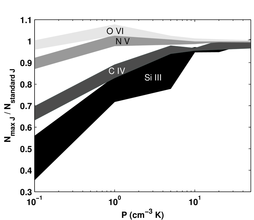
Figure 13.— The range of $N_{\rm max}/N_{\rm standard}$ ratios as a function of the external bounding pressure, for Si III, C IV, N V, and O VI produced in dwarf-scale-halos with $T=1-2\times 10^{6}$ K. Here $N_{\rm standard}$ are the columns computed with the standard field described in Section 2.2, and $N_{\rm max}$ are the columns computed with the maximal field, which is shallower above the Lyman limit. The high-ion columns are insensitive to spectral slope near the Lyman limit, and the intermediate-ions are only moderately affected, mostly for low bounding pressures.

Figure 13 compares the columns computed with the maximal field, $N_{\rm max}$, to the column computed with the standard field, $N_{\rm standard}$. We display the range of $N_{\rm max}/N_{\rm standard}$ ratios as a function of the external bounding pressure, for Si III, C IV, N V, and O VI produced in dwarf scale halos with $T=1-2\times 10^{6}$ K.

Figure 13 shows that for $P\gtrsim 1$ cm^-3 K, the O VI and N V columns remain similar, the C IV columns agree to within $20\%$, and the Si III columns agree to within $30\%$. For the lowest pressure that we consider, $P=0.1$ cm^-3 K, the differences are larger, but are still within a factor $2.5$. We conclude that column densities of the high ions are only weakly dependent on the exact spectral slope near the Lyman limit.

Table 5Column Densities for the Maximal Radiation Field

THIM	R	P/kB	$\sigma_{0}$		C IV	N V	O VI	Si III	Si IV	S III
$10^{6}$	$3$	$0.1$	85.62	central	$6.2\times 10^{9}$	$6.2\times 10^{9}$	$8.3\times 10^{10}$	$1.5\times 10^{5}$	$6.4\times 10^{6}$	$8.0\times 10^{4}$
				maximal	$2.6\times 10^{10}$	$1.8\times 10^{10}$	$1.9\times 10^{11}$	$1.0\times 10^{6}$	$4.1\times 10^{7}$	$3.6\times 10^{5}$
$10^{6}$	$3$	$1$	8.83	central	$1.4\times 10^{11}$	$4.9\times 10^{10}$	$3.9\times 10^{11}$	$4.1\times 10^{8}$	$3.3\times 10^{9}$	$2.0\times 10^{8}$
				maximal	$5.3\times 10^{11}$	$8.5\times 10^{10}$	$5.6\times 10^{11}$	$5.4\times 10^{9}$	$2.7\times 10^{10}$	$2.3\times 10^{9}$
$10^{6}$	$3$	$5$	1.81	central	$3.4\times 10^{11}$	$1.3\times 10^{11}$	$1.1\times 10^{12}$	$5.0\times 10^{9}$	$1.9\times 10^{10}$	$2.0\times 10^{9}$
				maximal	$1.2\times 10^{12}$	$2.8\times 10^{11}$	$2.0\times 10^{12}$	$9.6\times 10^{10}$	$1.5\times 10^{11}$	$3.4\times 10^{10}$
$10^{6}$	$3$	$10$	0.91	central	$4.3\times 10^{11}$	$1.7\times 10^{11}$	$1.7\times 10^{12}$	$1.1\times 10^{10}$	$2.7\times 10^{10}$	$5.1\times 10^{9}$
				maximal	$2.1\times 10^{12}$	$5.0\times 10^{11}$	$3.6\times 10^{12}$	$2.8\times 10^{11}$	$2.5\times 10^{11}$	$1.2\times 10^{11}$
$10^{6}$	$3$	$20$	0.46	central	$5.2\times 10^{11}$	$2.2\times 10^{11}$	$2.5\times 10^{12}$	$1.2\times 10^{10}$	$3.3\times 10^{10}$	$6.5\times 10^{9}$
				maximal	$3.6\times 10^{12}$	$8.5\times 10^{11}$	$6.2\times 10^{12}$	$3.6\times 10^{11}$	$4.4\times 10^{11}$	$1.7\times 10^{11}$
$10^{6}$	$3$	$50$	0.19	central	$7.1\times 10^{11}$	$3.4\times 10^{11}$	$4.5\times 10^{12}$	$5.3\times 10^{10}$	$4.6\times 10^{10}$	$3.0\times 10^{10}$
				maximal	$6.7\times 10^{12}$	$1.6\times 10^{12}$	$1.2\times 10^{13}$	$1.8\times 10^{12}$	$7.9\times 10^{11}$	$1.1\times 10^{12}$
$2\times 10^{6}$	$1.3$	$50$	3.34	central	$4.1\times 10^{11}$	$1.6\times 10^{11}$	$1.3\times 10^{12}$	$7.5\times 10^{9}$	$2.5\times 10^{10}$	$3.6\times 10^{9}$
				maximal	$2.5\times 10^{12}$	$5.4\times 10^{11}$	$3.2\times 10^{12}$	$2.3\times 10^{11}$	$3.3\times 10^{11}$	$1.0\times 10^{11}$
$2\times 10^{6}$	$3$	$0.1$	666.8	central	$5.4\times 10^{9}$	$5.6\times 10^{9}$	$6.9\times 10^{10}$	$1.3\times 10^{5}$	$4.9\times 10^{6}$	$7.1\times 10^{4}$
				maximal	$2.6\times 10^{10}$	$1.9\times 10^{10}$	$1.9\times 10^{11}$	$9.8\times 10^{5}$	$3.5\times 10^{7}$	$5.3\times 10^{5}$
$2\times 10^{6}$	$3$	$1$	68.70	central	$1.3\times 10^{11}$	$3.7\times 10^{10}$	$2.4\times 10^{11}$	$3.8\times 10^{8}$	$3.3\times 10^{9}$	$1.6\times 10^{8}$
				maximal	$4.4\times 10^{11}$	$6.5\times 10^{10}$	$3.2\times 10^{11}$	$4.3\times 10^{9}$	$2.4\times 10^{10}$	$1.5\times 10^{9}$
$2\times 10^{6}$	$3$	$5$	14.04	central	$3.0\times 10^{11}$	$9.0\times 10^{10}$	$6.2\times 10^{11}$	$4.6\times 10^{9}$	$1.7\times 10^{10}$	$1.7\times 10^{9}$
				maximal	$9.6\times 10^{11}$	$1.8\times 10^{11}$	$9.5\times 10^{11}$	$9.0\times 10^{10}$	$1.4\times 10^{11}$	$3.1\times 10^{10}$
$2\times 10^{6}$	$3$	$10$	7.08	central	$3.6\times 10^{11}$	$1.2\times 10^{11}$	$9.0\times 10^{11}$	$6.1\times 10^{9}$	$2.1\times 10^{10}$	$2.7\times 10^{9}$
				maximal	$1.5\times 10^{12}$	$3.0\times 10^{11}$	$1.6\times 10^{12}$	$1.5\times 10^{11}$	$1.9\times 10^{11}$	$6.4\times 10^{10}$
$2\times 10^{6}$	$3$	$20$	3.58	central	$4.1\times 10^{11}$	$1.5\times 10^{11}$	$1.3\times 10^{12}$	$1.6\times 10^{10}$	$2.6\times 10^{10}$	$7.7\times 10^{9}$
				maximal	$2.4\times 10^{12}$	$5.1\times 10^{11}$	$2.9\times 10^{12}$	$6.6\times 10^{11}$	$3.2\times 10^{11}$	$3.2\times 10^{11}$
$2\times 10^{6}$	$3$	$50$	1.45	central	$4.7\times 10^{11}$	$1.9\times 10^{11}$	$2.0\times 10^{12}$	$8.2\times 10^{9}$	$2.9\times 10^{10}$	$3.9\times 10^{9}$
				maximal	$4.7\times 10^{12}$	$1.1\times 10^{12}$	$6.8\times 10^{12}$	$3.6\times 10^{11}$	$6.0\times 10^{11}$	$1.6\times 10^{11}$
$2\times 10^{6}$	$7.5$	$0.1$	226.7	central	$7.7\times 10^{9}$	$8.6\times 10^{9}$	$1.1\times 10^{11}$	$1.8\times 10^{5}$	$6.7\times 10^{6}$	$1.0\times 10^{5}$
				maximal	$4.5\times 10^{10}$	$3.2\times 10^{10}$	$3.2\times 10^{11}$	$1.8\times 10^{6}$	$6.7\times 10^{7}$	$6.6\times 10^{5}$
$2\times 10^{6}$	$7.5$	$1$	27.48	central	$1.8\times 10^{11}$	$6.3\times 10^{10}$	$4.4\times 10^{11}$	$4.5\times 10^{8}$	$3.4\times 10^{9}$	$2.4\times 10^{8}$
				maximal	$9.5\times 10^{11}$	$1.5\times 10^{11}$	$6.2\times 10^{11}$	$8.8\times 10^{9}$	$4.2\times 10^{10}$	$4.1\times 10^{9}$
$2\times 10^{6}$	$7.5$	$5$	5.62	central	$3.7\times 10^{11}$	$1.3\times 10^{11}$	$1.0\times 10^{12}$	$6.3\times 10^{9}$	$1.9\times 10^{10}$	$2.8\times 10^{9}$
				maximal	$2.4\times 10^{12}$	$3.7\times 10^{11}$	$2.0\times 10^{12}$	$2.4\times 10^{11}$	$2.9\times 10^{11}$	$1.1\times 10^{11}$
$2\times 10^{6}$	$7.5$	$10$	2.83	central	$4.0\times 10^{11}$	$1.6\times 10^{11}$	$1.4\times 10^{12}$	$4.1\times 10^{9}$	$2.1\times 10^{10}$	$1.9\times 10^{9}$
				maximal	$2.8\times 10^{12}$	$6.0\times 10^{11}$	$3.6\times 10^{12}$	$1.6\times 10^{11}$	$3.2\times 10^{11}$	$6.9\times 10^{10}$
$2\times 10^{6}$	$7.5$	$20$	1.43	central	$4.7\times 10^{11}$	$1.9\times 10^{11}$	$1.9\times 10^{12}$	$1.9\times 10^{10}$	$3.1\times 10^{10}$	$9.2\times 10^{9}$
				maximal	$4.7\times 10^{12}$	$1.1\times 10^{12}$	$6.8\times 10^{12}$	$1.1\times 10^{12}$	$5.9\times 10^{11}$	$5.5\times 10^{11}$
$2\times 10^{6}$	$7.5$	$50$	0.58	central	$5.6\times 10^{11}$	$2.4\times 10^{11}$	$2.9\times 10^{12}$	$3.6\times 10^{10}$	$4.0\times 10^{10}$	$1.8\times 10^{10}$
				maximal	$9.5\times 10^{12}$	$2.1\times 10^{12}$	$1.5\times 10^{13}$	$2.4\times 10^{12}$	$1.2\times 10^{12}$	$1.3\times 10^{12}$
$10^{7}$	$3$	$10$	831.1	central	$3.7\times 10^{11}$	$1.3\times 10^{11}$	$9.8\times 10^{11}$	$7.0\times 10^{9}$	$1.7\times 10^{10}$	$2.5\times 10^{9}$
				maximal	$2.1\times 10^{12}$	$3.5\times 10^{11}$	$1.8\times 10^{12}$	$2.2\times 10^{11}$	$1.9\times 10^{11}$	$7.5\times 10^{10}$
$10^{7}$	$3$	$20$	419.3	central	$4.0\times 10^{11}$	$1.5\times 10^{11}$	$1.2\times 10^{12}$	$1.2\times 10^{10}$	$2.4\times 10^{10}$	$6.0\times 10^{9}$
				maximal	$2.4\times 10^{12}$	$4.9\times 10^{11}$	$2.6\times 10^{12}$	$6.1\times 10^{11}$	$3.1\times 10^{11}$	$3.0\times 10^{11}$
$10^{7}$	$3$	$50$	169.7	central	$4.3\times 10^{11}$	$1.7\times 10^{11}$	$1.5\times 10^{12}$	$7.5\times 10^{9}$	$2.5\times 10^{10}$	$3.4\times 10^{9}$
				maximal	$4.1\times 10^{12}$	$8.7\times 10^{11}$	$5.0\times 10^{12}$	$3.2\times 10^{11}$	$5.1\times 10^{11}$	$1.4\times 10^{11}$
$10^{7}$	$7.5$	$10$	332.4	central	$4.2\times 10^{11}$	$1.5\times 10^{11}$	$1.3\times 10^{12}$	$9.7\times 10^{9}$	$2.3\times 10^{10}$	$4.1\times 10^{9}$
				maximal	$3.2\times 10^{12}$	$5.7\times 10^{11}$	$3.1\times 10^{12}$	$4.2\times 10^{11}$	$3.7\times 10^{11}$	$1.7\times 10^{11}$
$10^{7}$	$7.5$	$20$	167.7	central	$4.4\times 10^{11}$	$1.7\times 10^{11}$	$1.5\times 10^{12}$	$1.5\times 10^{10}$	$2.7\times 10^{10}$	$6.7\times 10^{9}$
				maximal	$4.1\times 10^{12}$	$8.8\times 10^{11}$	$5.0\times 10^{12}$	$8.4\times 10^{11}$	$5.2\times 10^{11}$	$3.7\times 10^{11}$
$10^{7}$	$7.5$	$50$	67.88	central	$4.6\times 10^{11}$	$1.8\times 10^{11}$	$1.7\times 10^{12}$	$2.3\times 10^{10}$	$3.0\times 10^{10}$	$1.0\times 10^{10}$
				maximal	$7.0\times 10^{12}$	$1.5\times 10^{12}$	$9.1\times 10^{12}$	$1.7\times 10^{12}$	$9.2\times 10^{11}$	$7.4\times 10^{11}$

Note. — Assuming $\phi_{s}=0.3$. Columns were computed for $Z=0.1$ times solar, and are proportional to $Z$.

Electronic (only) Figure Set 8

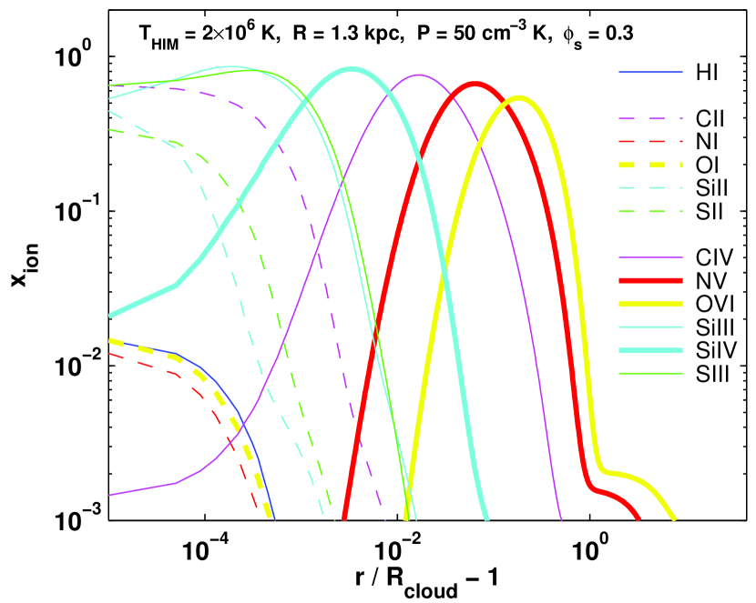
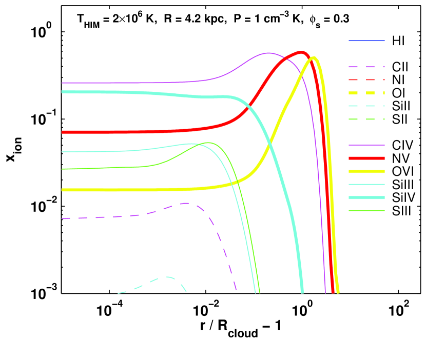
Figure 8.1, 8.2.— Ion fractions as a function of scaled radius $r/R-1$, in conductive interfaces surrounding dwarf galaxy-scale halos. The ambient temperature, $T_{\rm HIM}$, cloud radius, $R$, and bounding pressure, $P$ are indicated in each panel.

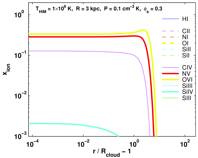
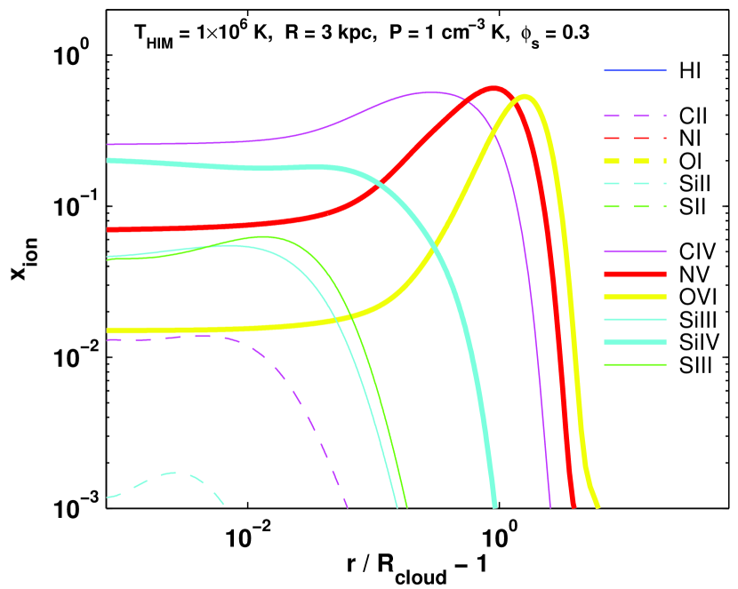
Figure 8.3, 8.4.— Ion fractions versus scaled radius in dwarf galaxy-scale models – continued.

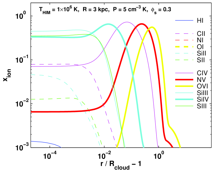
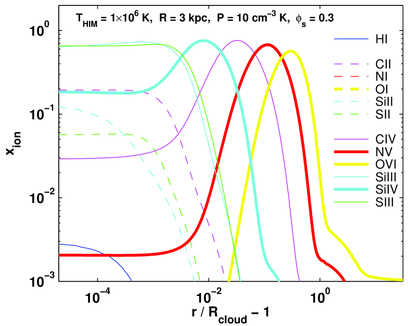
Figure 8.5, 8.6.— Ion fractions versus scaled radius in dwarf galaxy-scale models – continued.

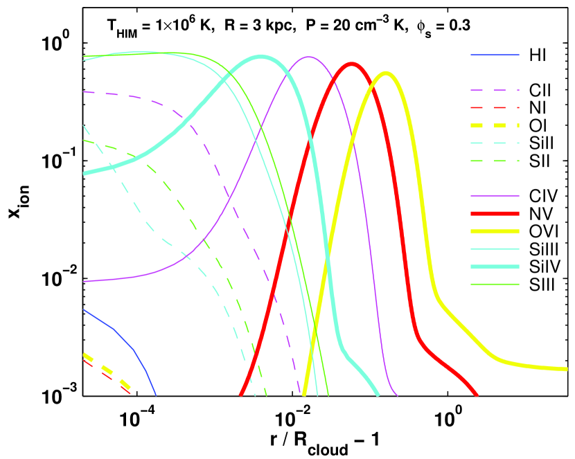
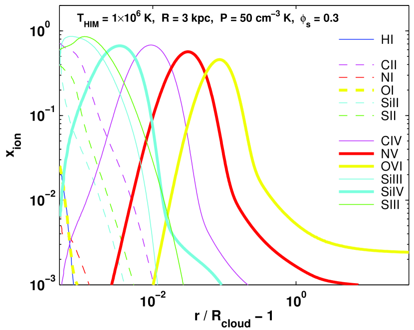
Figure 8.7, 8.8.— Ion fractions versus scaled radius in dwarf galaxy-scale models – continued.

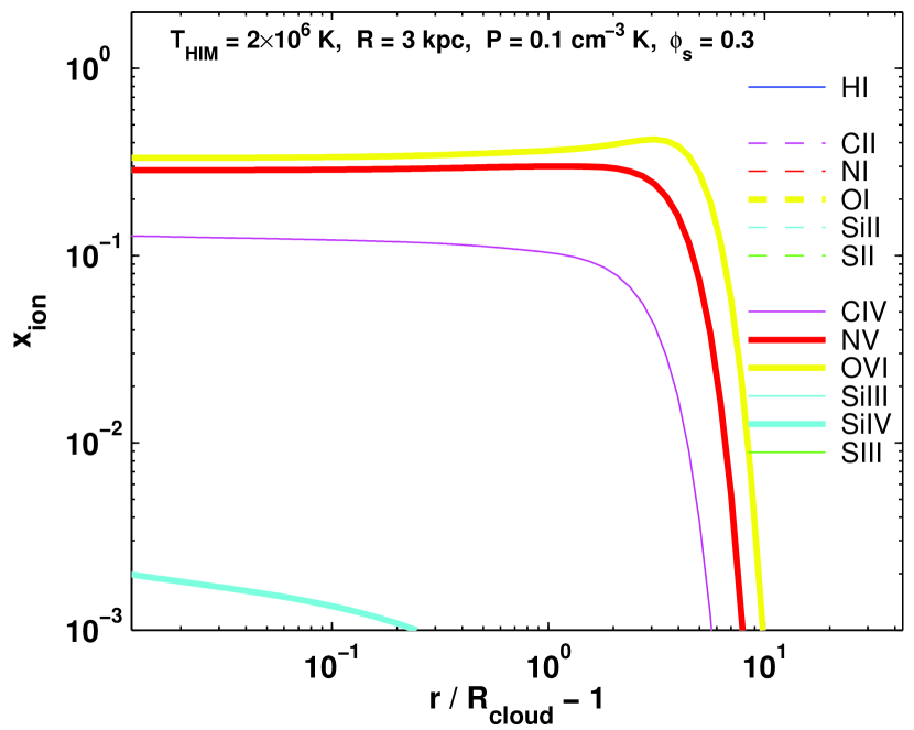
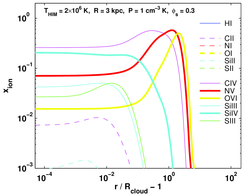
Figure 8.9, 8.10.— Ion fractions versus scaled radius in dwarf galaxy-scale models – continued.

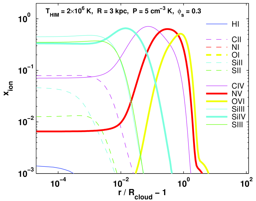
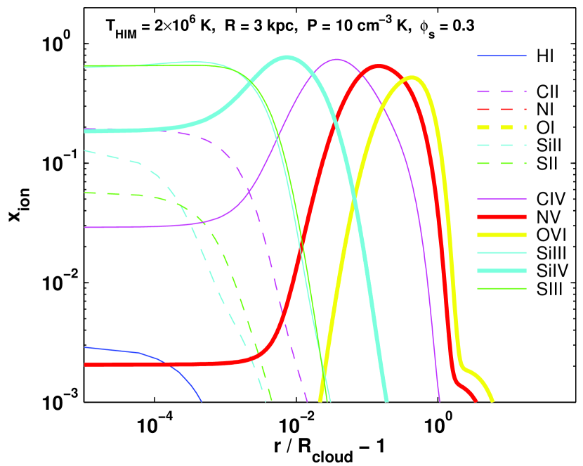
Figure 8.11, 8.12.— Ion fractions versus scaled radius in dwarf galaxy-scale models – continued.

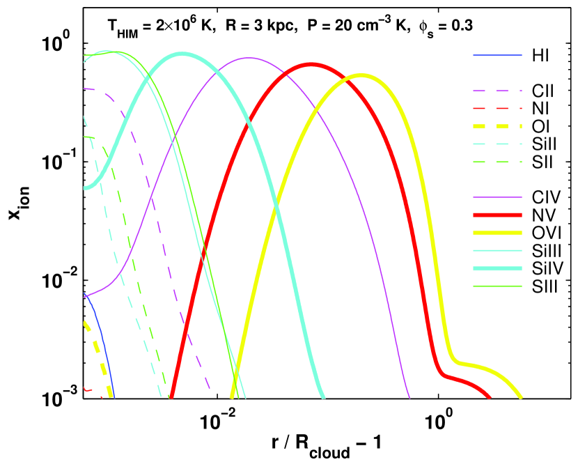
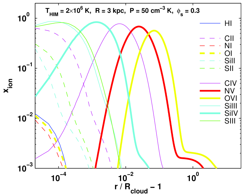
Figure 8.13, 8.14.— Ion fractions versus scaled radius in dwarf galaxy-scale models – continued.

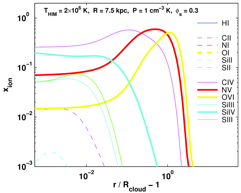
Figure 8.15, 8.16.— Ion fractions versus scaled radius in dwarf galaxy-scale models – continued.

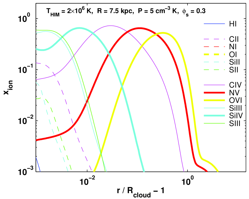
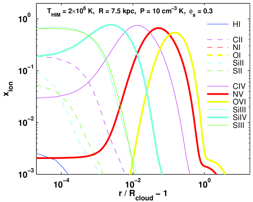
Figure 8.17, 8.18.— Ion fractions versus scaled radius in dwarf galaxy-scale models – continued.

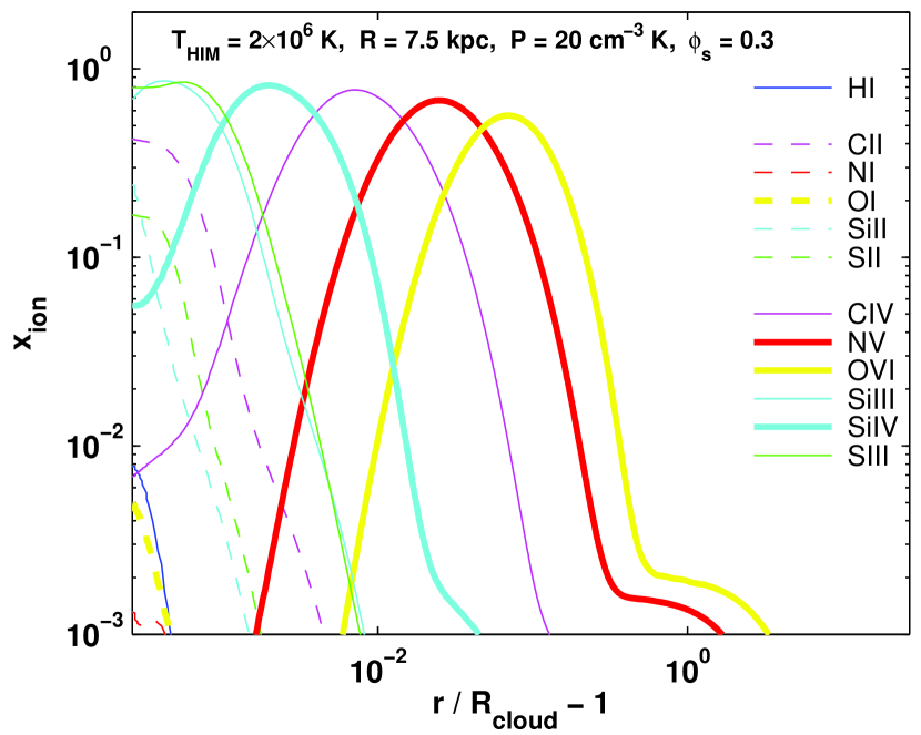
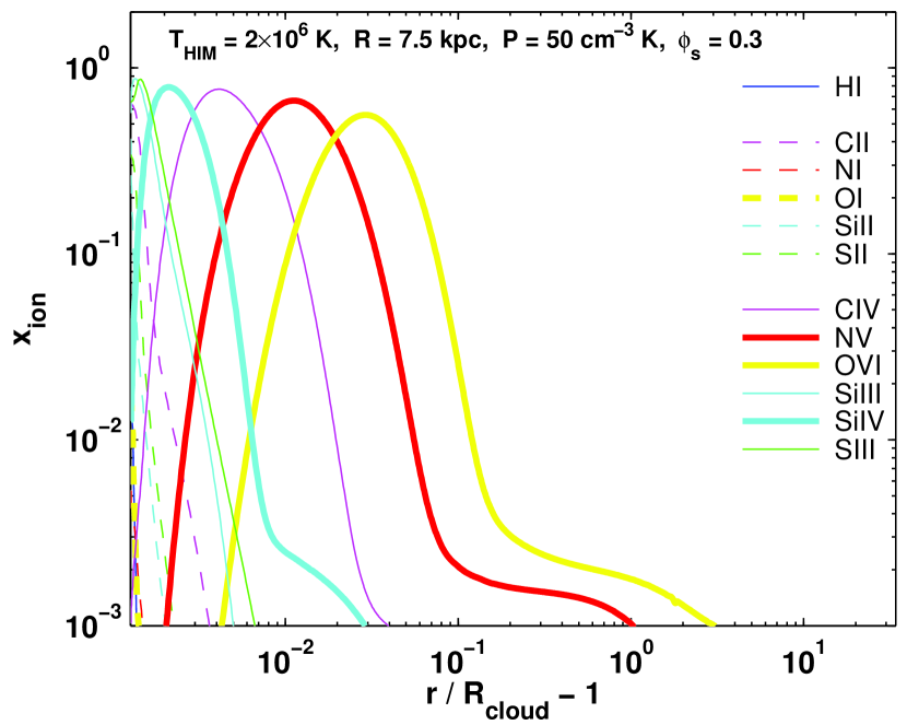
Figure 8.19, 8.20.— Ion fractions versus scaled radius in dwarf galaxy-scale models – continued.

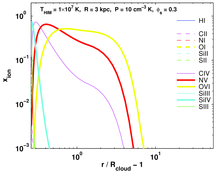
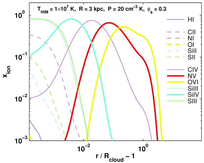
Figure 8.21, 8.22.— Ion fractions versus scaled radius in dwarf galaxy-scale models – continued.

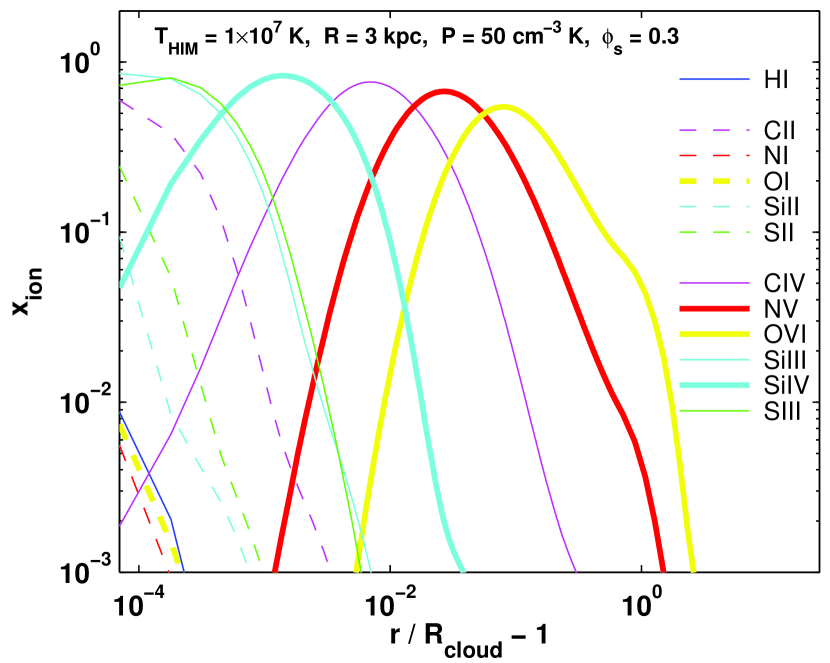
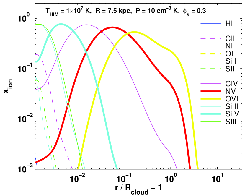
Figure 8.23, 8.24.— Ion fractions versus scaled radius in dwarf galaxy-scale models – continued.

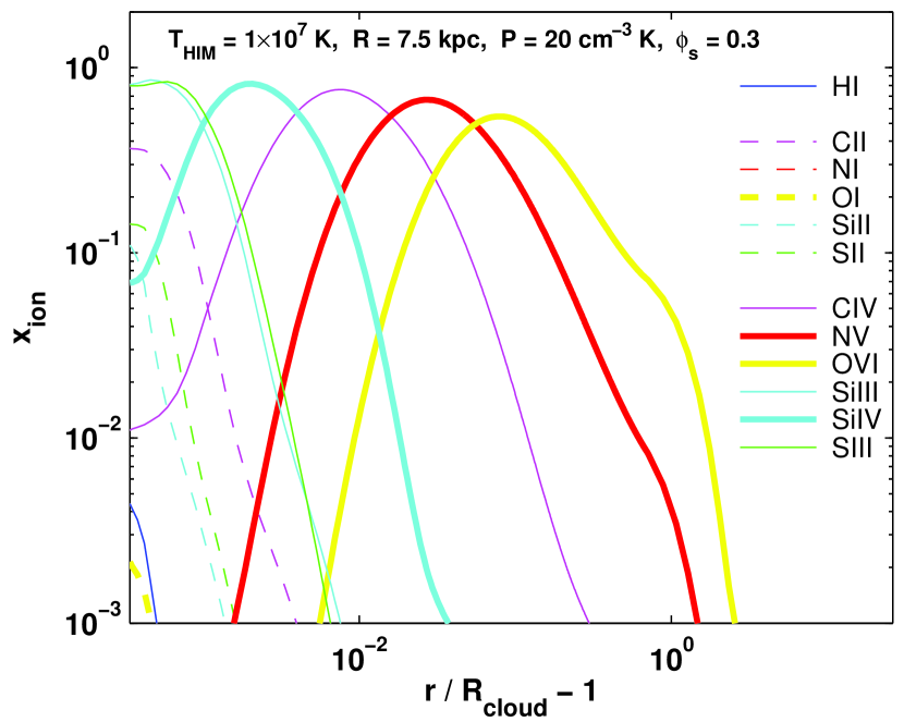
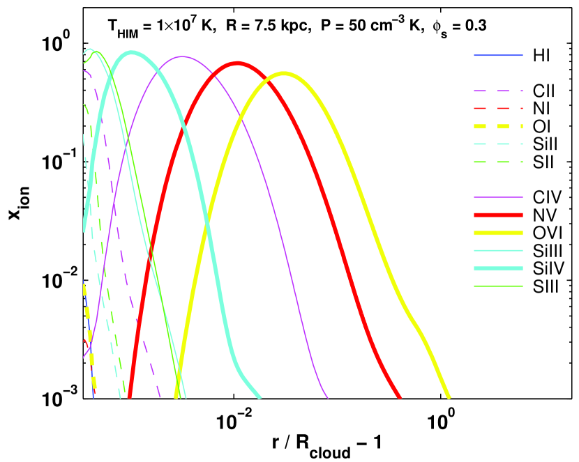
Figure 8.25, 8.26.— Ion fractions versus scaled radius in dwarf galaxy-scale models – continued.

References

- Aldrovandi & Pequignot (1973) Aldrovandi, S. M. V., & Pequignot, D. 1973, A&A, 25, 137
- Allen et al. (2008) Allen, M. G., Groves, B. A., Dopita, M. A., Sutherland, R. S., & Kewley, L. J. 2008, ApJS, 178, 20
- Altun et al. (2006) Altun, Z., Yumak, A., Badnell, N. R., Loch, S. D., & Pindzola, M. S. 2006, A&A, 447, 1165
- Altun et al. (2005) Altun, Z., Yumak, A., Badnell, N. R., Colgan, J., & Pindzola, M. S. 2005, A&A, 433, 395
- Altun et al. (2004) Altun, Z., Yumak, A., Badnell, N. R., Colgan, J., & Pindzola, M. S. 2004, A&A, 420, 775
- Arnaud & Raymond (1992) Arnaud, M., & Raymond, J. 1992, ApJ, 398, 394
- Arnaud & Rothenflug (1985) Arnaud, M., & Rothenflug, R. 1985, A&AS, 60, 425
- Badnell (2006) Badnell, N. R. 2006, A&A, 447, 389
- Badnell et al. (2003) Badnell, N. R., et al. 2003, A&A, 406, 1151
- Balbus & McKee (1982) Balbus, S. A., & McKee, C. F. 1982, ApJ, 252, 529
- Ballet et al. (1986) Ballet, J., Arnaud, M., & Rothenflug, R. 1986, A&A, 161, 12
- Balsara et al. (2008) Balsara, D. S., Bendinelli, A. J., Tilley, D. A., Massari, A. R., & Howk, J. C. 2008, MNRAS, 386, 642
- Bernstein, Freedman, & Madore (2002) Bernstein, R. A., Freedman, W. L., & Madore, B. F. 2002, ApJ, 571, 56
- Boehringer & Hartquist (1987) Boehringer, H., & Hartquist, T. W. 1987, MNRAS, 228, 915
- Borkowski et al. (1990) Borkowski, K. J., Balbus, S. A., & Fristrom, C. C. 1990, ApJ, 355, 501
- Chen, Fabian, & Gendreau (1997) Chen, L.-W., Fabian, A. C., & Gendreau, K. C. 1997, MNRAS, 285, 449
- Clarke et al. (1998) Clarke, N.J., et al. 1998, J. Phys. B: At. Mol. Opt. Phys. 33, 533
- Colgan et al. (2005) Colgan, J., Pindzola, M. S., & Badnell, N. R. 2005, A&A, 429, 369
- Colgan et al. (2004) Colgan, J., Pindzola, M. S., & Badnell, N. R. 2004, A&A, 417, 1183
- Colgan et al. (2003) Colgan, J., Pindzola, M. S., Whiteford, A. D., & Badnell, N. R. 2003, A&A, 412, 597
- Collins et al. (2009) Collins, J. A., Shull, J. M., & Giroux, M. L. 2009, ApJ, 705, 962
- Collins et al. (2007) Collins, J. A., Shull, J. M., & Giroux, M. L. 2007, ApJ, 657, 271
- Collins et al. (2005) Collins, J. A., Shull, J. M., & Giroux, M. L. 2005, ApJ, 623, 196
- Collins et al. (2004) Collins, J. A., Shull, J. M., & Giroux, M. L. 2004, ApJ, 605, 216
- Collins et al. (2003) Collins, J. A., Shull, J. M., & Giroux, M. L. 2003, ApJ, 585, 336
- Cowie & McKee (1977) Cowie, L. L., & McKee, C. F. 1977, ApJ, 211, 135
- Dalton & Balbus (1993) Dalton, W. W., & Balbus, S. A. 1993, ApJ, 404, 625
- Edgar & Chevalier (1986) Edgar, R. J., & Chevalier, R. A. 1986, ApJ, 310, L27
- Fang et al. (2006) Fang, T., Mckee, C. F., Canizares, C. R., & Wolfire, M. 2006, ApJ, 644, 174
- Faucher-Giguère et al. (2009) Faucher-Giguère, C.-A., Lidz, A., Zaldarriaga, M., & Hernquist, L. 2009, ApJ, 703, 1416
- Ferland et al. (1998) Ferland, G. J., Korista, K. T., Verner, D. A., Ferguson, J. W., Kingdon, J. B., & Verner, E. M. 1998, PASP, 110, 761
- Ferland et al. (1997) Ferland, G. J., Korista, K. T., Verner, D. A., & Dalgarno, A. 1997, ApJ, 481, L115
- Fox et al. (2006) Fox, A. J., Savage, B. D., & Wakker, B. P. 2006, ApJS, 165, 229
- Fox et al. (2005) Fox, A. J., Wakker, B. P., Savage, B. D., Tripp, T. M., Sembach, K. R., & Bland-Hawthorn, J. 2005, ApJ, 630, 332
- Fox et al. (2004) Fox, A. J., Savage, B. D., Wakker, B. P., Richter, P., Sembach, K. R., & Tripp, T. M. 2004, ApJ, 602, 738
- Giovanelli et al. (2010) Giovanelli, R., Haynes, M. P., Kent, B. R., & Adams, E. A. K. 2010, ApJ, 708, L22
- Gnat & Sternberg (2009) Gnat, O., & Sternberg, A. 2009, ApJ, 693, 1514
- Gnat & Sternberg (2007) Gnat, O., & Sternberg, A. 2007, ApJS, 168, 213
- Gnat & Sternberg (2004) Gnat, O., & Sternberg, A. 2004, ApJ, 608, 229
- Haardt & Madau (1996) Haardt, F. & Madau, P. 1996, ApJ, 461, 20
- Heckman et al. (2002) Heckman, T. M., Norman, C. A., Strickland, D. K., & Sembach, K. R. 2002, ApJ, 577, 691
- Hindmarsh (1983) Hindmarsh, A. C., 1983, ODEPACK, A Systematized Collection of ODE Solvers, in Scientific Computing, R. S. Stepleman et al. (eds.), North-Holland, Amsterdam, 1983 (vol. 1 of IMACS Transactions on Scientific Computation), pp. 55-64.
- Jenkins (2009) Jenkins, E. B. 2009, Space Science Reviews, 143, 205
- Kepner et al. (1999) Kepner, J., Tripp, T. M., Abel, T., & Spergel, D. 1999, AJ, 117, 2063
- Kingdon & Ferland (1996) Kingdon, J. B., & Ferland, G. J. 1996, ApJS, 106, 205
- Landini & Fossi (1991) Landini, M., & Fossi, B. C. M. 1991, A&AS, 91, 183
- Landini & Monsignori Fossi (1990) Landini, M., & Monsignori Fossi, B. C. 1990, A&AS, 82, 229
- Martin, Hurwitz, & Bowyer (1991) Martin, C., Hurwitz, M., & Bowyer, S. 1991, ApJ, 379, 549
- McKee & Begelman (1990) McKee, C. F., & Begelman, M. C. 1990, ApJ, 358, 392
- McKee & Cowie (1977) McKee, C. F., & Cowie, L. L. 1977, ApJ, 215, 213
- Mitnik & Badnell (2004) Mitnik, D. M., & Badnell, N. R. 2004, A&A, 425, 1153
- Murphy et al. (2000) Murphy, E. M. et al. 2000, ApJ, 538, L35
- McCray (1987) McCray, R. 1987, in Spectroscopy of Astrophysical Plasmas, Eds. A. Dalgarno & D. Layzer (Cambridge University Press), p. 255
- Nagashima et al. (2007) Nagashima, M., Inutsuka, S., & Koyama, H. 2007, SINS - Small Ionized and Neutral Structures in the Diffuse Interstellar Medium, 365, 121
- Narayanan et al. (2010) Narayanan, A., et al. 2010, American Astronomical Society Meeting Abstracts, 215, #460.05
- Nipoti & Binney (2007) Nipoti, C., & Binney, J. 2007, MNRAS, 382, 1481
- Pequignot et al. (1991) Pequignot, D., Petitjean, P., & Boisson, C. 1991, A&A, 251, 680
- Savage & Lehner (2006) Savage, B. D., & Lehner, N. 2006, ApJS, 162, 134
- Savage et al. (2005) Savage, B. D., Lehner, N., Wakker, B. P., Sembach, K. R., & Tripp, T. M. 2005, ApJ, 626, 776
- Scott et al. (2004) Scott, J. E., Kriss, G. A., Brotherton, M., Green, R. F., Hutchings, J., Shull, J. M., & Zheng, W. 2004, ApJ, 615, 135
- Sembach et al. (2003) Sembach, K. R. et al. 2003, ApJS, 146, 165
- Sembach, Gibson, Fenner, & Putman (2002) Sembach, K. R., Gibson, B. K., Fenner, Y., & Putman, M. E. 2002, ApJ, 572, 178
- Sembach et al. (2000) Sembach, K. R. et al. 2000, ApJL, 538, L31
- Sembach, Savage, Lu, & Murphy (1999) Sembach, K. R., Savage, B. D., Lu, L., & Murphy, E. M. 1999, ApJ, 515, 108
- Shelton (1998) Shelton, R. L. 1998, ApJ, 504, 785
- Shull et al. (2009) Shull, J. M., Jones, J. R., Danforth, C. W., & Collins, J. A. 2009, ApJ, 699, 754
- Shull et al. (2004) Shull, J. M., Tumlinson, J., Giroux, M. L., Kriss, G. A., & Reimers, D. 2004, ApJ, 600, 570
- Shull et al. (1999) Shull, J. M., Roberts, D., Giroux, M. L., Penton, S. V., & Fardal, M. A. 1999, AJ, 118, 1450
- Shull & van Steenberg (1982) Shull, J. M., & van Steenberg, M. 1982, ApJS, 48, 95
- Slavin (2007) Slavin, J. D. 2007, SINS - Small Ionized and Neutral Structures in the Diffuse Interstellar Medium, 365, 113
- Slavin (1989) Slavin, J. D. 1989, ApJ, 346, 718
- Slavin & Cox (1992) Slavin, J. D., & Cox, D. P. 1992, ApJ, 392, 131
- Slavin & Frisch (2002) Slavin, J. D. & Frisch, P. C. 2002, ApJ, 565, 364
- Smith & Cox (2001) Smith, R. K. & Cox, D. P. 2001, ApJS, 134, 283
- Spitzer (1962) Spitzer, L. 1962, Physics of Fully Ionized Gases, New York: Interscience (2nd edition), 1962,
- Stancil et al. (1998) Stancil, P. C., et al. 1998, ApJ, 502, 1006
- Sternberg et al. (2002) Sternberg, A., McKee, C. F., & Wolfire, M. G. 2002, ApJS, 143, 419
- Stocke et al. (2006) Stocke, J. T., Penton, S. V., Danforth, C. W., Shull, J. M., Tumlinson, J., & McLin, K. M. 2006, ApJ, 641, 217
- Sutherland & Dopita (1993) Sutherland, R. S., & Dopita, M. A. 1993, ApJS, 88, 253
- Telfer et al. (2002) Telfer, R. C., Zheng, W., Kriss, G. A., & Davidsen, A. F. 2002, ApJ, 565, 773
- Tufte et al. (2002) Tufte, S. L., Wilson, J. D., Madsen, G. J., Haffner, L. M., & Reynolds, R. J. 2002, ApJ, 572, L153
- Tumlinson et al. (2005) Tumlinson, J., Shull, J. M., Giroux, M. L., & Stocke, J. T. 2005, ApJ, 620, 95
- Verner et al. (1996) Verner, D. A., Ferland, G. J., Korista, K. T., & Yakovlev, D. G. 1996, ApJ, 465, 487
- Vieser & Hensler (2007) Vieser, W., & Hensler, G. 2007, A&A, 475, 251
- Voronov (1997) Voronov, G. S. 1997, Atomic Data and Nuclear Data Tables, 65, 1
- Wakker et al. (2003) Wakker, B. P. et al. 2003, ApJS, 146, 1
- Zatsarinny et al. (2006) Zatsarinny, O., Gorczyca, T. W., Fu, J., Korista, K. T., Badnell, N. R., & Savin, D. W. 2006, A&A, 447, 379
- Zatsarinny et al. (2005) Zatsarinny, O., Gorczyca, T. W., Korista, K. T., Fu, J., Badnell, N. R., Mitthumsiri, W., & Savin, D. W. 2005a, A&A, 438, 743
- Zatsarinny et al. (2005) Zatsarinny, O., Gorczyca, T. W., Korista, K. T., Fu, J., Badnell, N. R., Mitthumsiri, W., & Savin, D. W. 2005b, A&A, 440, 1203
- Zatsarinny et al. (2004) Zatsarinny, O., Gorczyca, T. W., Korista, K., Badnell, N. R., & Savin, D. W. 2004b, A&A, 426, 699
- Zatsarinny et al. (2004) Zatsarinny, O., Gorczyca, T. W., Korista, K. T., Badnell, N. R., & Savin, D. W. 2004a, A&A, 417, 1173
- Zatsarinny et al. (2003) Zatsarinny, O., Gorczyca, T. W., Korista, K. T., Badnell, N. R., & Savin, D. W. 2003, A&A, 412, 587
- Zheng et al. (2004) Zheng, W., et al. 2004, ApJ, 605, 631