Three carbon-enhanced metal-poor dwarf stars from the SDSS

Abstract

Context. The origin of carbon-enhanced metal-poor stars enriched with both $s$ and $r$ elements is highly debated. Detailed abundances of these types of stars are crucial to understand the nature of their progenitors.

Aims. The aim of this investigation is to study in detail the abundances of SDSS J1349-0229, SDSS J0912+0216 and SDSS J1036+1212, three dwarf CEMP stars, selected from the Sloan Digital Sky Survey.

Methods. Using high resolution VLT/UVES spectra (R $\sim 30\,000$) we determine abundances for Li, C, N, O, Na, Mg, Al, Ca, Sc, Ti, Cr, Mn, Fe, Co, Ni and 21 neutron-capture elements. We made use of CO⁵BOLD 3D hydrodynamical model atmospheres in the analysis of the carbon, nitrogen and oxygen abundances. NLTE corrections for Ci and Oi lines were computed using the Kiel code.

Results. We classify SDSS J1349-0229 and SDSS J0912+0216 as CEMP-r+s stars. SDSS J1036+1212 belongs to the class CEMP-no/s, with enhanced Ba, but deficient Sr, of which it is the third member discovered to date. Radial-velocity variations have been observed in SDSS J1349-0229, providing evidence that it is a member of a binary system.

Conclusions. The chemical composition of the three stars is generally compatible with mass transfer from an AGB companion. However, many details remain difficult to explain. Most notably of those are the abundance of Li at the level of the Spite plateau in SDSS J1036+1212 and the large over-abundance of the pure r-process element Eu in all three stars.

1 Introduction

Carbon-enhanced metal-poor (hereafter CEMP) stars owe their name to a considerable overabundance of carbon with respect to iron ([C/Fe] $>$ +1.0), and represent a sizeable fraction of the very metal-poor stars ([Fe/H] $<$ –2.0). The frequency of CEMP stars has been estimated to be of the order of 14% by Cohen et al. (2005) and of 21% by Lucatello et al. (2006). This frequency appears to increase with decreasing metallicity, reaching approximately 40% for stars with [Fe/H] $<$ –3.5 (Beers & Christlieb 2005). The carbon excess in CEMP stars may stem from carbon production by nucleosynthesis in an asymptotic giant branch (AGB) star followed by mass transfer to a surviving companion. An alternative mechanism is the formation of the star from a C-enriched interstellar medium.

The chemical composition of these stars shows a considerable variety. On the basis of the abundance pattern of neutron capture elements Beers & Christlieb (2005) suggested to divide CEMP stars into four classes: CEMP-no, CEMP-s, CEMP-r/s, CEMP-r. To these classes Sivarani et al. (2006) proposed to add the class of CEMP-no/s to accommodate two stars discovered in the course of the “First Stars” programme (see Bonifacio et al. 2009a, and references therein for a description of the programme).

The CEMP-no stars do not show any enhancement of neutron-capture elements. The prototype of this class is CS 22957-027 (Norris et al. 1997; Bonifacio et al. 1998). The class also includes the three most Fe-poor stars known: HE 0107-5240, HE 1327-2326 and HE 0557-4840 (Christlieb et al. 2002; Frebel et al. 2005; Norris et al. 2007).

The majority of CEMP stars with [Fe/H] $>-3$ are strongly enhanced in $s$-process elements (Aoki et al. 2007) and form the class CEMP-s. Radial-velocity studies by Lucatello et al. (2005) have shown that these may all be members of binary systems, providing strong evidence for the mass transfer scenario from a more massive companion. The large scatter of observed $s$-element abundances may arise from the different masses of the companion stars, which presents a useful constraint for AGB nucleosynthesis models.

Among the stars with strong enhancement of the $s$-process elements, a high percentage also show large enhancements of $r$-process elements. These stars belong to the class CEMP-r/s, the prototypes of which (CS 22948-27 and CS 29497-34) were first studied by Barbuy et al. (1997) and Hill et al. (2000). Many scenarios have been proposed to explain the observed abundances. Most involve two independant processes, one for the $r$-elements and one for the $s$-elements. None of the scenarios, however, is entirely convincing given the many different abundance patterns observed in r/s stars as well as the uncertainties regarding the astrophysical sites of the r-process. For example, Johnson & Bolte (2004) find r-element ratios which are difficult to explain with combinations of the normal r and s-processes.

Only one r-process enhanced CEMP star (CEMP-r) has been detected: CS 22892-052 (Sneden et al. 2003). This stars exhibits the lowest carbon enhancement of all CEMP stars: [C/Fe] = +1.0. The $r$-process pattern observed in the heavier n-capture elements was found to be in excellent agreement with the scaled solar $r$-process abundances. Lighter elements with 40 $\leq$ Z $\leq$ 50 however were not found to match, leading the authors to suggest the existence of two $r$-process sites.

Finally the class of CEMP-no/s was up to now defined by only two members, CS 29528-041 and CS 31080-095, which show an enhancement of Ba over iron of about 1 dex, but a sizeable underabundance of Sr.

The diversity of $s$ and $r$-element patterns among CEMP stars strongly suggests that this population of stars has several astrophysical origins. Other mechanisms may be responsible for their nucleosynthetic history beyond those involving AGB stars. Since the $s$-process and $r$-process occur under different physical conditions, they are likely to arise in different astrophysical sites.

In this paper we present detailed abundance analyses of three dwarf CEMP stars: SDSS J1349-0229, SDSS J0912+0216 and SDSS J1036+1212. These stars are extremely metal-poor, with [Fe/H] $<$ –2.50, and were selected from our ongoing survey of extremely metal-poor dwarf candidates from the Sloan Digital Sky Survey. The first two belong to the CEMP-r+s class, while the third is the third known example of a CEMP-no/s star, after the first two discovered by Sivarani et al. (2006), suggesting that the class is probably not so rare.

Table 1: Log of observations.

Star	$\alpha$              $\delta$	Date & Time	Exposure	Setting	Heliocentric	$g$
			time		radial velocity
	(J2000)	yyyy-mm-dd  UT	(s)		$\mathrm{km\leavevmode\nobreak\ s}^{-1}$	mag
SDSS J1349-0229	13 49 13.5 –02 29 42.8	2007-01-31 07:32:54	3800	Dic1 390+580	92.3	16.63
		2009-04-15 02:24:25	3005	Dic2 346+760	121.8	16.63
		2009-04-15 03:54:58	3005	Dic2 346+760	121.7	16.63
		2009-04-15 04:52:57	3005	Dic2 346+760	122.0	16.63
		2009-04-15 05:45:07	3005	Dic2 346+760	122.4	16.63
SDSS J0912+0216	09 12 43.7 +02 16 23.7	2006-12-31 07:41:05	3005	Dic1 390+580	138.0	15.67
SDSS J1036+1212	10 36 49.9 +12 12 19.8	2007-01-29 07:16:27	3005	Dic1 390+580	–47.9	16.59

2 Target selection and observations

We selected extremely metal-poor (EMP) dwarf candidates from the Sloan Digital Sky Survey (SDSS; York et al. 2000; Adelman-McCarthy et al. 2007, 2008) with an automatic analysis code (Bonifacio & Caffau 2003) in a version which provides estimates of [M/H] from low resolution spectra. These candidates were observed at high resolution with the UVES spectrograph (Dekker et al. 2000) at the ESO 8.2m Kueyen-VLT telescope as part of our survey of stars at low metallicity.

We observed 17 candidates; among these were the objects SDSS J1349-0229, SDSS J0912+0216 and SDSS J1036+1212. The SDSS spectra showed strong $G$ bands in these stars, and the weakness of the Ca ii K lines indicated very low metallicities. Figure 1 displays the prominent CH G band of all three stars. This band is hardly detectable in non-C-enhanced stars of this effective temperature and metallicity. We thus targeted the three objects as CEMP stars. An analysis of the remaining 14 candidates will be presented in a future paper (Bonifacio et al. 2010).

The slit was set to 1$\aas@@fstack{\prime\prime}$4 and the detector was read with a $2\times 2$ on-chip binning. The resulting resolution is $R\sim 30\,000$. Supplementary observations were obtained for SDSS J1349-0229 in the ESO period 83 to study the UV OH lines and the permitted O i triplet at 777 nm. Details on the settings and exposure times are listed in Table 1 along with measurements of the radial velocities. The second epoch observation of SDSS J1349-0229 reveals a large radial-velocity variation of the order of 30 $\mathrm{km\leavevmode\nobreak\ s}^{-1}$, indicating clearly that it is a member of a binary system. The signal-to-noise ratio varies from 35 at 392 nm up to 110 above 650 nm.

Figure 1: Observed UVES spectra of the CH G band in the three CEMP stars. Spectra have been offset for clarity.

3 Atmospheric parameters

The effective temperatures of the stars were determined using both the wings of H$\alpha$ and the Fe i excitation equilibrium. The surface gravity was derived from the Fe i/Fe ii ionisation equilibrium, while the microturbulence was determined from Fe i lines. The FITLINE code (François et al. 2003) was used to measure the equivalent widths of the Fe i and Fe ii lines. ATLAS model atmospheres and SYNTHE (Kurucz 1993, 2005b) synthetic spectra in their Linux version (Sbordone et al. 2004, Sbordone 2005) have been employed in the analysis, using scaled solar abundances with the exception of the alpha-elements, which were enhanced by 0.4 dex. The opacity distribution functions of Castelli & Kurucz (2003) with a microturbulence of 1 $\mathrm{km\leavevmode\nobreak\ s}^{-1}$have been used. The H$\alpha$ profiles were computed using the ATLAS9 models and a modified version of the BALMER code. The self-broadening of H$\alpha$ was treated with the Barklem et al. (2000, 2000b) theory, and for the Stark broadening the computations of Stehlé & Hutcheon (1999) were used. Adopted stellar parameters are listed in Table 2.

The carbon and nitrogen abundances are significantly enhanced in these stars. In order to investigate the impact of the carbon abundance on the atmospheric structure, models were computed for our stellar parameters using ATLAS12 (Kurucz 1996, 2005a; Castelli 2005) with a carbon enhancement of +3.0 dex, and a nitrogen enhancement of +2.0 dex. The average temperature difference in the two temperature structures is of the order of 20 K. This small change in the temperature distribution translates into an error of approximately 0.02 dex in the abundance determination. The analysis was therefore performed using the ATLAS9 models.

Table 2: Adopted stellar parameters.

Star	$T_{\rm eff}$	log $g$	$\xi$	[Fe/H]
	K	cgs	$\mathrm{km\leavevmode\nobreak\ s}^{-1}$	dex
SDSS J1349-0229	6200	4.0	1.5	–3.0
SDSS J0912+0216	6500	4.5	1.5	–2.5
SDSS J1036+1212	6000	4.0	1.4	–3.2

4 Abundances

The majority of the elemental abundances presented were determined by the equivalent widths of unblended lines. A 1D LTE analysis was performed with the WIDTH9 code (Kurucz 1993, 2005a; Castelli 2005). The van der Waals damping constants have been taken from the Kurucz data base when available. When not available SYNTHE uses the WIDTH approximation (see Castelli 2005b and also Ryan 1998). Abundances of strong lines, blended lines, or lines that are affected by hyperfine structure were treated by line-profile fitting, using the same code as in Caffau et al. (2005). The mean LTE 1D abundance for each of the 35 elements investigated in the three stars in our sample are presented in Table 3. In each line of the table we provide an estimate of the error for each star. For abundance indicators with multiple lines this is simply the standard deviation of the abundances derived from individual lines. For complex molecular bands like C₂ the error has been estimated from the $\chi^{2}$ of the best fitting synthetic spectrum. The systematic errors for changes in effective temperature and surface gravity are similar to those of Sivarani et al. (2006): 0.10–0.15  dex in [X/Fe] for a change of 100 K in effective temperature or 0.5 dex in log $g$. As a reference we adopted the solar abundances derived with the use of the CO⁵BOLD solar model, when available (Caffau et al. 2009), for other elements we adopted the values of Lodders (2003).

Table 3: Elemental abundances for the three CEMP stars obtained from an analysis using 1D stellar atmospheres.

	SDSSJ1349-0229			SDSSJ0912+0216			SDSSJ1036+1212			Sun
Element	log($\epsilon$)	[X/Fe]	$\sigma$	log($\epsilon$)	[X/Fe]	$\sigma$	log($\epsilon$)	[X/Fe]	$\sigma$	log($\epsilon$)
Li							2.21
C(CH)	8.32	2.82	0.05	8.17	2.17	0.03	6.77	1.47	0.10	8.50
C(C2)	8.66	3.16	0.02							8.50
C(C i) NLTE	7.92	2.42	0.11	7.38	1.38	0.05				8.50
N(NH)	6.46	1.60	0.12	7.11	1.75	0.12	5.95	1.29	0.25	7.86
O(OH)	7.64	1.88	0.10							8.76
O(O i) NLTE	7.39	1.63	0.14							8.76
Na i NLTE	4.79	1.49	0.01	4.18	0.38	0.03	3.53	0.43	0.01	6.30
Mg i	5.12	0.57	0.16	5.26	0.21	0.13	4.35	0.00	0.06	7.55
Al i NLTE	3.51	0.11	…	4.08	0.18	…	3.24	0.04	…	6.46
Ca i	3.74	0.40	0.08	3.32	0.42	0.12	3.52	0.38	0.17	6.34
Sc ii	0.08	0.01	…	0.85	0.28	…	–0.02	0.11	0.15	3.07
Ti i				2.96	0.54	0.03				4.92
Ti ii	2.47	0.55	0.09	2.93	0.51	0.18	2.47	0.75	0.26	4.92
Cr i	2.61	–0.02	0.21	2.99	–0.16	0.06	2.33	–0.12	0.17	5.65
Cr ii	2.82	0.17	…	3.07	–0.08	0.21	2.43	–0.02	0.30	5.65
Mn i	1.82	–0.68	0.08	2.45	–0.55	…				5.50
Mn ii				2.49	–0.51	0.03	1.84	–0.46	0.20	5.50
Co i	2.24	0.33	0.19	2.72	0.31	0.15	2.28	0.57	0.09	4.91
Ni i	3.48	0.26	0.37	3.79	0.07	0.18	3.30	0.28	0.22	6.22
Sr ii	1.21	1.30	0.17	0.98	0.57	0.07	–0.85	–0.56	0.04	2.91
Y ii	0.49	1.29	0.29	0.31	0.61	0.20	–0.76	0.24	0.43	2.20
Zr ii	1.16	1.56	0.32	1.18	1.08	0.17	0.42	1.02	0.17	2.60
Ru i				1.93	2.61	…				1.82
Pd i							0.90	2.40	0.19	1.70
Ba ii	1.35	2.17	0.12	1.17	1.49	0.08	0.15	1.17	0.15	2.18
La ii	–0.08	1.74	0.05	0.03	1.35	0.14	0.37	2.39	0.60	1.18
Ce ii	1.24	2.63	0.11	1.28	2.17	0.14	0.73	2.32	0.41	1.61
Pr ii	0.65	2.87	0.07	0.53	2.25	0.13	0.03	2.45	0.11	0.78
Nd ii	0.37	1.91	0.12	0.08	1.12	0.31	0.35	2.08	0.36	1.46
Sm ii	0.30	2.35	0.01	1.05	2.60	0.08	0.67	2.92	0.15	0.95
Eu ii	–0.86	1.62	0.08	–0.78	1.20	0.05	–1.42	1.26	0.24	0.52
Gd ii	0.56	2.50	0.23	1.36	2.80	0.08	0.48	2.62	0.44	1.06
Tb ii	0.00	2.69	0.40	0.46	2.64	0.36	0.01	2.90	0.24	0.31
Dy ii	0.52	2.39	0.17	0.59	1.96	0.13	0.39	2.46	0.34	1.13
Er ii	0.68	2.73	0.08	0.48	2.03	0.23	0.61	2.86	0.04	0.95
Tm ii							–0.31	2.78	0.13	0.11
Hf ii	1.01	3.14	…	1.09	2.72	0.19	0.02	2.35	0.60	0.87
Os ii							0.28	2.11	…	1.37
Ir i							0.15	2.00	…	1.35
Pb i	2.14	3.09	…	1.88	2.33	0.30				2.05

It is known that convection in metal-poor stars induces very low temperatures in the outermost layers, which are not predicted by classical 1D stellar atmospheres (Asplund et al. 1999; Collet et al. 2007; Caffau & Ludwig 2007; González Hernández et al. 2008), this behaviour is often referred to as “overcooling”. This is particularly important for molecular lines, which form high up in the atmosphere, where the overcooling is largest. Investigations of CH, NH and OH abundances in dwarf atmospheres with [Fe/H] = –2.0 by Asplund (2004) have shown that 1D models tend to overestimate abundances by more than 0.3 dex when compared to 3D hydrodynamical simulations. Collet et al. (2007) performed a similar investigation with red giant stars at [Fe/H] = –3.0 and found the corrections for CH, NH and OH to be in the range of –0.5 to –1.0 dex.

It is thus mandatory to use 3D hydrodynamical simulations to assess molecular abundances in metal-poor stars. For this purpose, we employed 3D model atmospheres computed with the CO⁵BOLD code (Freytag et al. 2002; Wedemeyer et al. 2004). The 3D spectral synthesis calculations were performed with the code Linfor3D. The parameters of the 3D models used in the analysis are listed in Table 4. The models were chosen from our 3D model grid (Ludwig et al. 2009) to best correspond with the stellar parameters of our three stars. Since we did not have a 3D model with [Fe/H] = –2.5, we interpolated for SDSS J0912+0216 between the corrections obtained from the models with [Fe/H] = –2.0 and –3.0 (d3t65g45mm20n01 & d3t65g45mm30n01).

For each full 3D model, Linfor3D computes a temporal and horizontal average of the 3D structure over surfaces of equal (Rosseland) optical depth (hereafter denoted as $\left\langle\mathrm{3D}\right\rangle$). We compared the abundances derived from each of our 3D models to this average model $\left\langle\mathrm{3D}\right\rangle$ and to a corresponding standard hydrostatic 1D model atmosphere (1D_LHD). The 1D_LHD models are calculated assuming plane-parallel geometry and employ the same micro-physics (equation-of-state, opacities) as CO⁵BOLD. Convection is described by a mixing-length theory in the formulation of Mihalas (1978); the adopted mixing-length-parameter was 0.5.

Two main effects distinguish 3D models from 1D models: the average temperature profile and the horizontal temperature fluctuations. The contribution of both effects is quantified by the 3D correction in the sense 3D – 1D. The correction attributed solely to the horizontal temperature fluctuations is denoted by 3D – $\left\langle\mathrm{3D}\right\rangle$. A complete description of 3D corrections is given by Caffau et al. (2008) and references therein.

4.1 Lithium

The Li i 670.7 nm doublet was detected in SDSS J1036+1212, and an abundance of A(Li) = 2.21 was derived. The doublet is not detected in SDSS J1349-0229 and SDSS J0912+0216.

Table 4: Parameters of 3D models used in the analysis.

Model	$T_{\rm eff}$	log $g$	[Fe/H]
d3t63g40mm30n01	6270	4.00	–3.0
d3t65g45mm20n01	6530	4.50	–2.0
d3t65g45mm30n01	6550	4.50	–3.0
d3t59g40mm30n02	5850	4.00	–3.0

The abundance of Li determined is quite high for this type of star, but “normal” for dwarf stars of this metallicity. In 2002, Reyniers et al. presented an alternative identification of the Li doublet in post-AGB stars: a Ce ii line. Since SDSS J1036+1212 is strongly enhanced in neutron-capture elements (see Sect. 4.8), we investigated this possibility. The observed line is plotted in Fig. 2. Synthetic spectra were calculated with the abundance of Sm ii and Ce ii listed in Table 3 and three abundances of lithium: log $\epsilon$ = 1.00, 2.00 and 2.21.

Figure 2: Observed and synthetic spectra of SDSS J1036+1212 in the region of the Li i 670.7 nm doublet. Nearby lines of Ce ii and Sm ii were included in the synthesis. Synthetic spectra are shown with lithium abundances of $\epsilon$ = 1.00, 2.00 and 2.21. See the text for details.

Even with a significant enhancement, the contribution of the Sm ii and Ce ii lines are minimal. A stronger contribution from these lines would require a much lower surface gravity at this temperature. Additionally, we do not find that the line is shifted redwards compared to nearby lines, as was the case for the AGB stars of Reyniers et al. (2002). We can therefore confirm the identification of the observed feature with the Li i resonance doublet and a lithium abundance of 2.21 for this star at our stellar parameters.

4.2 Carbon

Although in principle the carbon abundance of CEMP stars may be determined from both molecular and atomic lines, the majority of the values cited in the literature are derived from spectral lines of CH in the $G$ band, as these are strong features in CEMP star spectra. In some cases C₂ features and Ci lines may be present. We detect CH, C₂ and Ci lines in SDSS J1349-0229 and CH and Ci lines in SDSS J0912+0216. These stars exhibit a very strong carbon enhancement. In SDSS J1036+1212, the carbon enhancement is much weaker, and only CH lines could be used to determine [C/Fe]. The results are summarised in Table 5.

In order to perform 3D spectrum synthesis of molecular lines, which are computationally demanding, we decided to focus on four isolated CH features at 416.4 nm, 416.9 nm, 418.0 nm, and 418.8 nm to determine [C/Fe] in all three stars. The line data were taken from the molecular line lists of Kurucz (Kurucz 2005b), but the oscillator strengths were scaled by a factor of 0.4, as was done by Bonifacio et al. (1998) to place the log $gf$ values on the same scale as the ones by Norris et al. (1997). From our 1D analysis we obtain [C/Fe] = 2.82 $\pm$ 0.05, 2.17 $\pm$ 0.03 and 1.47 $\pm$ 0.10 for SDSS J1349-0229, SDSS J0912+0216 and SDSS J1036+1212, respectively. The 3D corrections for these lines are quite substantial, have the effect to reduce the carbon abundance, and range from –0.73 to –0.50 dex.

A 1D carbon abundance of [C/Fe] = 3.16 was derived from C₂ features at 516.3 nm in the spectrum of SDSS J1349-0229. As for CH, we used the molecular line lists of Kurucz (Kurucz 2005b) for the C₂ lines. The 3D correction was computed from a synthesis of 118 lines centered at 516.3 nm and spanning 0.6 nm. Observed and synthetic spectra of the feature are shown in Fig. 3. The 3D corrections for this feature are much more substantial than the corrections for the CH lines, they even reach –1.44 dex. This is because the C₂ lines form in layers which are more superficial than those where the CH lines form, where the effects of overcooling and photospheric inhomogeneities are strongest.

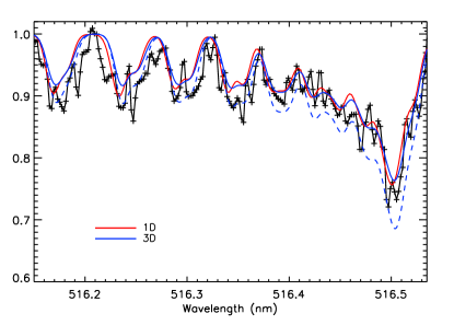
Figure 3: Observed and 1D and 3D synthetic spectra of SDSS J1349-0229 in the region of the C₂ band at 516.3 nm. The 3D spectra was computed with [C/Fe]=1.72 while the 1D spectra was computed with [C/Fe]=3.16. The dashed line shows the 3D synthetic spectra with an increase of 0.15 dex in carbon abundance.

Three Ci lines were measured in SDSS J1349-0229 and two in SDSS J0912+0216. All of these lines are high excitation lines, and are highly sensitive to NLTE effects. Using LTE largely overestimates the abundance. The 3D corrections on the other hand, show that the 1D abundance is underestimated, however by a very small amount, the largest corrections being 0.08 dex. NLTE corrections were calculated using the Kiel code (Steenbock & Holweger 1984) and the carbon model atom described in Stürenburg & Holweger (1990), and are listed in Table 6. The effects of collisions with hydrogen atoms were treated as described in Steenbock & Holweger (1984), who generalised the Drawin (1969) formalism. We provide NLTE corrections for three different values of S_H, a scaling factor, S${}_{H}=0$ means totally neglecting collisions with H atoms, while S${}_{H}=1$ means taking the value of the Steenbock & Holweger (1984) formalism. The NLTE Ci abundance listed in Table 5 adopts the NLTE corrections for S_H=1/3.

The three abundance indicators for SDSS J1349-0229 do not give consistent results either in the 1D or in the 3D analysis. The standard deviations of the abundances from the different features are 0.30 and 0.32 from the 1D and the 3D analyses, respectively. In 1D the most significant difference occurs between the C₂ and Ci lines, where we find a difference of 0.74 dex. In 3D the biggest difference of 0.79 dex occurs between the Ci and C₂ lines. The Ci lines give a much higher abundance. Meanwhile the difference between 3D CH and Ci is 0.42 dex, assuming an S_H=1/3. For SDSS J0912+0216, where only CH and Ci lines are available, we find differences of 0.79 and 0.23 dex and $\sigma$ = 0.40 and 0.12 in 1D and 3D, respectively.

The sensitivity of the molecular lines to temperature is clear from the significant 3D corrections. In Fig. 4 we have plotted the temperature distributions for the 3D, $\left\langle\mathrm{3D}\right\rangle$, and 1D_LHD models. The ranges of the depth of formation, intended as the range in optical depth over which the line contribution function is significantly different from zero, of the CH, C₂ and Ci lines are overplotted as horizontal lines. In 1D we derive a larger C abundance from the C₂ lines than from the CH lines, while in 3D the reverse is true. This can be understood by looking at the different depths of formation of the C₂ and CH lines in the 1D and 3D models. The C₂ lines are formed higher up in the atmosphere compared to the CH lines, but far more in the 3D model than in the 1D. The 3D models do not achieve a better consistency between CH and C₂ lines. The C i lines are quite insensitive to 3D effects. Neither in 3D nor in 1D we achieved consistent results between molecular lines and Ci.

In view of the high formation region of C₂ we must consider the validity of the models in this region of the atmosphere. The 3D model properties, like the choice of the opacity binning scheme, may well have an effect on the structure of the outer regions of the atmosphere. To explore this effect, we recomputed the carbon 3D corrections for SDSS J1349-0229 with a 3D model atmosphere that employs 12 opacity bins versus the six bins used in the models listed in Table 4. The 3D corrections are compared in Table 7. The 12 bin model gives a better agreement between the CH the C₂ lines, and both molecular features appear agree better with C i. Although these results appear encouraging, the formation region of the C₂ lines is quite high and at low density. The validity of LTE for molecule formation and levels population may well be an oversimplification. For further discussion on this topic see Behara et al. (2009).

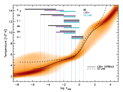
Figure 4: The temperature structure for the 3D model d3t63g40mm30n01 is plotted as a function of $\tau_{\rm ross}$ along with the average 3D ($\left\langle\mathrm{3D}\right\rangle$) and the corresponding 1D_lHD temperature structures. Overplotted on the figure are the ranges of the depth of formation of the C₂, CH, Ci, NH, OH and Oi spectral lines used in the analysis.

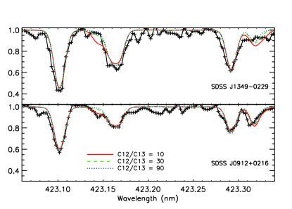
Figure 5: Observed and synthetic spectra for two stars in the region of the ¹³CH and ¹²CH lines. Solid, dashed and dotted lines show the synthetic spectrum with a ratio of ¹²C/¹³C = 10, 30 and 90 respectively.

4.2.1 The ¹²C/¹³C ratio

CH features from the $R$-branch of the $A^{2}\Delta-X^{2}\Pi$ band were used in our analysis of the ¹²C/¹³C isotopic ratio. Only lower limits could be derived: 30 for SDSS J1349-0229, and 10 for SDSS J0912+0216. Observed spectra and fits to synthetic spectra are shown in Fig. 5. The low carbon abundance of SDSS J1036+1212 prevented us from obtaining a lower limit to the ¹²C/¹³C isotopic ratio.

4.3 Nitrogen

We obtain the nitrogen abundances for the three stars from isolated NH features at $\sim$ 336 nm. We used the Kurucz data (Kurucz 2005b) for the NH molecule in our analysis, and following Spite et al. (2005) applied a correction of –0.40 dex to our abundances. The 1D analysis yields [N/Fe] = 1.60, 1.75 and 1.29 for SDSS J1349-0229, SDSS J0912+0216 and SDSS J1036+1212 respectively. The magnitude of the 3D corrections for NH is greater than the corrections for CH in all three stars and follows the same direction by reducing the 1D abundance. The corrections range from –0.67 to –0.93. The adopted 3D abundances are listed in Table 5.

4.4 Oxygen

The oxygen forbidden lines at 630.0 and 636.4 nm are not detected in the spectra of our stars. Measured upper limits range from [O/Fe] = 2.0 to 2.5 for the three stars. Spectra in the range of the UV OH lines and the permitted O i triplet at 777 nm were only available for SDSS J1349-0229, and therefore we can only determine the oxygen abundance for this star. We computed the abundance from three isolated UV OH lines of the (0-0) vibrational band of the $A^{2}\Sigma-X^{2}\Pi$ electronic systems, and computed the corresponding 3D corrections. The $gf$ values of the OH lines were computed from the lifetimes calculated by Goldman & Gillis (1981). The result is [O/Fe] = 1.70. We obtained a higher abundance from the triplet lines: [O/Fe] = 1.81. However, it is well known that these high excitation lines suffer from NLTE effects (see e.g. Gratton et al. 1999 and references therein). We computed NLTE corrections using the Kiel code (Steenbock & Holweger 1984) and the model-atom described in Paunzen et al. (1999). For oxygen the collisions with hydrogen atoms were treated with the Steenbock & Holweger (1984) formalism for three choices of S_H. The corrections are listed in Table 6. Taking this into account, we obtained an abundance from the triplet lines of 1.69, which agrees excellently with the abundance obtained from the OH lines.

The 3D corrections for the OH lines are quite low ($\sim-0.2$) compared to values found in the literature for metal-poor stars: Asplund & García Pérez (2001) state values of less than –0.60 dex, and González Hernández et al. (2008) obtain corrections of –1.50 dex for dwarfs stars with [Fe/H] = –3.00. The 3D corrections for OH lines are very sensitive to the C/O ratio in the atmosphere. We fixed [C/O] = 1.00 in our calculations. Using a solar carbon-to-oxygen ratio yields a correction of –1.35 dex. Figure 6 shows the contribution function for a line computed for the two different C/O ratios. When carbon is enhanced, there is no contribution to the OH line higher in the atmosphere, since the oxygen is tied up in CO in this region due to the high carbon content.

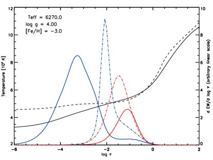
Figure 6: Equivalent width contribution function plotted as a function of optical depth for the 3D model (blue) and the 1D_LHD model (red) for two different C/O ratios. Scaled solar carbon-to-oxygen is plotted as a solid line, while [C/O] = 1 is plotted as a dot-dashed line. Overplotted are the temporal and horizontal average of the temperature profile of the 3D model (black solid line) and the temperature profile of the 1D_LHD model (dashed black line).

Table 5: Carbon, nitrogen and oxygen abundances and 3D corrections. Abundances are expressed with respect to the solar abundances of log ($\epsilon$) = 8.50, 7.86, and 8.76 for carbon, nitrogen and oxygen, respectively.

Element	[X/Fe]1D	[X/Fe]3D	3D–1D	3D–$\left\langle\mathrm{3D}\right\rangle$
	SDSS J1349-0229
CH	2.82	2.09	–0.73	–0.37
C2	3.16	1.72	–1.44	–0.82
C i NLTE	2.42	2.51	0.08	–0.04
NH	1.60	0.67	–0.93	–0.34
OH	1.88	1.70	–0.18	–0.06
O i NLTE	1.63	1.69	0.06	–0.04
	SDSS J0912+0216
CH	2.17	1.67	–0.50	–0.20
C i NLTE	1.38	1.44	0.06	–0.03
NH	1.75	1.07	–0.67	–0.30
	SDSS J1036+1212
CH	1.47	0.96	–0.51	–0.11
NH	1.29	0.51	–0.78	–0.08

Table 6: NLTE corrections for carbon and oxygen lines.

Line (nm)	SH = 1.0	SH = 1/3	SH = 0.0
	SDSS J1349-0229
C i 493.2	–0.352	–0.432	–0.502
C i 505.2	–0.369	–0.456	–0.535
C i 538.0	–0.379	–0.468	–0.543
O i 777.1	–0.127	–0.144	–0.130
O i 777.4	–0.098	–0.111	–0.099
O i 777.5	–0.100	–0.113	–0.101
	SDSS J0912+0216
C i 505.2	–0.267	–0.352	–0.456
C i 658.8	–0.258	–0.335	–0.425

Table 7: 3D corrections calculated using 6 and 12 opacity bins.

3D model	CH	C2	C i NLTE
6 bin [X/Fe]3D	2.09	1.72	2.51
12 bin [X/Fe]3D	2.22	1.99	2.50

4.5 The alpha elements (Z $>$ 8)

Our measurements of [Mg/Fe], [Ca/Fe] and [Ti/Fe] in all three stars yield results that are consistent with the majority of metal-poor stars (Cayrel et al. 2004; Bonifacio et al. 2009b).

4.6 The odd-Z elements

Our measurement of [Na/Fe] was made using the Na D resonance lines at 588.995 and 589.592 nm. We have applied NLTE corrections from Gratton et al. (1999). The corrections range from –0.07 to –0.15 dex. All stars show an enhancement of Na, which is typical for CEMP stars (Stancliffe 2009).

The abundance of Al was measured from the 396.152 nm line. We found [Al/Fe] to be nearly solar in all three stars after applying the NLTE correction from Baumüller & Gehren (1997) of +0.64, the mean value given for stars with [Fe/H] $<$ –2.20 in their Table 2. This correction agrees closely with the NLTE correction given by Andrievsky et al. (2008) of 0.6 dex for stars with [Fe/H] = –3.00.

4.7 The iron-peak elements

The values of [Sc/Fe], [Mn/Fe] and [Co/Fe] all agree with typical values for metal-poor stars (Cayrel et al. 2004; Bonifacio et al. 2009b). The abundance of Mn and Co were calculated using spectrum synthesis to take the effects of hyperfine splitting (HFS) into account. In the analysis we adopt the hfs line lists of Kurucz (2005b).

We were able to measure Cr i and Cr ii lines in all stars. The abundances derived from the Cr ii lines were found to be systematically higher than the values obtained from the Cr i lines. Bonifacio et al. (2009b) already noted this behaviour and suggested it may be due to NLTE effects. On average, we found a difference of 0.12 dex. The results of Cr i are consistent with the wide range of reported Cr abundances from CEMP stars though.

We note that Bergemann (2008) and Bergemann & Gehren (2009) suggest that Mn, Co and Cr are affected by significant NLTE effects although no computations exist yet at a metallicity of –3. In any case these corrections will be similar for CEMP stars and “normal” stars.

A wide range of [Ni/Fe] values are found in CEMP stars. All our stars show an enhancement of Ni, which ranges from +0.07 to +0.28 dex.

4.8 Neutron-capture elements

The spectra of all three stars display a wealth of neutron-capture element lines. All in all 21 elements are detected. Pb is detected in two stars, while in the third, SDSS J1036+1212, third peak r-process elements are detected.

We derive strontium abundances for our stars employing the strong Sr ii 407.7 nm and 421.5 nm lines shown in Fig. 7. SDSS J1349-0229 and SDSS J0912+0216 exhibit overabundances of Sr of 1.30 and 0.57 dex, while SDSS J1036+1212 shows an underabundance of Sr by 0.56 dex. Zirconium and yttrium are found to be enriched in all stars.

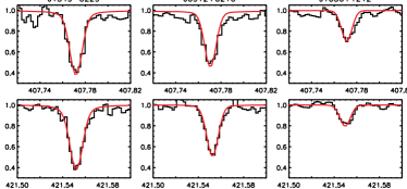
Figure 7: Sr ii 407.7 nm and 421.5 nm lines used in the abundance analysis.

Barium is overabundant in all three stars, although slightly less so in SDSS J1036+1212. The Ba abundances were estimated from the Ba ii 493.4 nm and 614.1 nm lines. For the analysis we adopted the HFS by McWilliam (1998) and assumed a solar isotopic mix. We note however that if a pure $r$-process isotopic mix is assumed, the barium abundance is decreased by 0.1 to 0.35 dex.

Abundances from lanthanum lines were derived in all stars with the hyperfine structure constants and transition probabilities from Lawler et al. (2001a). The HFS components were calculated by the code LINESTRUC (Wahlgren 2005).

For the cerium abundance analysis we adopted the line list from Lawler et al. (2009). The praseodymium abundance was derived using line lists from Li et al. (2007) and Ivarsson et al. (2001). Since the lines are relatively weak, we ignored any HFS. The linelist from Den Hartog et al. (2003) was used to determine the neodymium abundance.

For the analysis of the samarium lines we applied the values from Lawler et al. (2006). Europium lines were detected in all stars, and abundances were determined with the help of spectrum synthesis and line profile fitting, taking into account the HFS. Gadolinium line data were taken from Den Hartog et al. (2006), and data for terbium from Lawler et al. (2001b).

We ignored HFS in dypsrosium as the lines were weak. Oscillator strengths were adopted from Wickliffe et al. (2000). Data for erbium lines were taken from Lawler et al. (2008). For thulium we used the data from Wickliffe & Lawler (1997). The effects due to HFS are small and were ignored. For the analysis of hafnium, we adopted values from Lawler et al. (2007).

Osmium and iridium lines were detected only in SDSS J1036+1212. Lead was detected in SDSS J1349-0229 and SDSS J0912+0216. The line list from Aoki et al. (2002) was used in the analysis.

5 Comparison with similar stars

It is now widely accepted that the CEMP class includes objects which have rather diverse astrophysical origin. In Sect. 1 we described the classification scheme proposed by Beers & Christlieb (2005) based on the abundances of neutron-capture elements in CEMP stars. This classification is non-quantitative in the sense that one refers loosely to “enhancement” of $r$ or $s$-process elements without specifying which ones, and without providing quantitative limits for the enhancements. In the note to their Table 4, Sivarani et al. (2006) attempted to provide a more quantitative description of the classes, based essentially on the abundance of Ba and for one class (CEMP-s) also on the Ba/Eu ratio.

Jonsell et al. (2006) defined the class CEMP-r+s, which is different from the class CEMP-r/s of Beers & Christlieb (2005). In Table 8 we provide the definitions found in the literature of the different classes. All stars are assumed to have [C/Fe]$>+1$.

Table 8: Classification of CEMP stars based on abundances of neutron-capture elements. S2006 and J2006 refer to Sivarani et al. (2006) and Jonsell et al. (2006), respectively.

Class	Definition	Reference
CEMP-no	[Ba/Fe]$<0.0$	S2006
CEMP-no/s	$+0.5<$[Ba/Fe]$<+1.0$	S2006
CEMP-s	[Ba/Fe]$>+1.0$ & [Ba/Eu]$>+0.5$	S2006
CEMP-s	[Ba/Fe]$>+1.0$ & [Ba/Eu]$>+0.0$	J2006
	& [Eu/Fe] $<+1.0$
CEMP-r/s	$0.0<$[Ba/Fe]$<+0.5$	S2006
CEMP-r+s	[Ba/Fe] $>$ 1.0 & [Eu/Fe] $>$ 1.0	J2006

The classification scheme above is phenomenological and also leaves space for some ambiguity. For instance, all three of our programme stars belong to the CEMP-r+s class, but SDSS J1349-0229 also classifies as a CEMP-s (S2006) star. Moreover the really striking characteristic of the CEMP-no/s stars is that [Ba/Fe]$>0$ and [Sr/Fe]$<0$; if we redefine the class in this way, then SDSS J1036+1212 would classify as a CEMP-no/s star. Although our preferred carbon, nitrogen and oxygen abundances are those derived from the 3D analysis, we adopt the abundances from the 1D analysis to compare our stars with a sample of hot dwarf CEMP stars from the literature. The full sample of stars selected is compiled from Table 10 of Aoki et al. (2008), Table 8 of Jonsell et al. (2006) and Table 4 of Sivarani et al. (2006).

5.1 Lithium

Few values of lithium have been measured in CEMP stars. Often only upper limits can be measured. Due to its fragility this element is an excellent diagnostic of the thermal history of the material. It is easily destroyed at temperatures above $2.5\times 10^{6}$ K, therefore material which has experienced these temperatures should be essentially Li-free. This could explain why CEMP stars generally show no Li, as the temperatures necessary to produce the carbon will lead to Li destruction.

Still, a few CEMP stars have been observed to have Li values close to the value of the Spite plateau (Spite & Spite 1982a, b). We present a sample of measured abundances in Fig. 8. A few stars show Li at the Spite plateau level, while others show a lower Li abundance. A remarkable example is the double lined spectroscopic binary CS 22964-161 (Thompson et al. 2008). The two stars are both CEMP, the primary is a warm sub-giant, while the secondary is a main sequence star. Li has been measured at the level of the Spite plateau in the primary star and is only tentatively detected in the secondary, again close to the Spite plateau. If binary mass transfer is responsible for the abundances of this system, it must once have been a triple system. That Li is detected at all in a star polluted by nuclearly processed material is in itself surprising, that it should be at the level of the Spite plateau is even more. There could of course be a conspiracy in a way that the Li produced in the donor star exactly matches the destroyed Li, modulo the dilution factor of the accreted material. In the case of CS 22964-161 one further requires that the dilution factor has been very nearly the same for both components of the binary. Lithium may be produced via several mechanisms during the AGB phase. However, if the observed lithium originates from the donor star, the question arises why Li abundances above the Spite plateau have not been detected.

We observe a Li abundance corresponding to the Spite plateau in SDSS J1036+1212. A scenario alternative to mass transfer in a binary star to explain the observed abundances would be the formation of SDSS J1036+1212 from a cloud of C-rich material. Also in this case the C-rich material should be essentially Li-free though, thus the Li-puzzle remains. Radial velocity monitoring of this star would be highly desirable to constrain the existence of a binary companion.

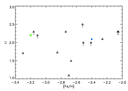
Figure 8: Abundance of lithium as a function of [Fe/H]. Abundances from literature are plotted as open triangles, while the star symbol is from this work. The filled circle shows CS 22964-161.

5.2 Carbon and nitrogen

We plot [C/H] as a function of [Fe/H] in Fig. 9. The open symbols are from the literature, while the star symbols are from this work. Excluding three objects, SDSS J1036+1212 (this work), CS 29528-041 (Sivarani et al. 2006) and CS 22964-161 (Thompson et al. 2008), the stars display a rather constant [C/H], slightly less than solar. A possible explanation is that such a roughly constant value is found when the accretion from the AGB star occurs through Roche lobe overflow. This suggests that the AGB companion always provides basically the same mass of carbon and the accretion mode through Roche lobe overflow ensures a roughly constant dilution factor. In this scenario stars with low carbon abundance, like SDSS J1036+1212, CS 29528-041 and CS 22964-161 would arise through AGB wind instead from accretion, which implies larger dilution fractions.

There are three problems with this scenario: the first is that one would expect the plane [C/H], [Fe/H] to be almost uniformly populated with different efficiencies due to a mixture of cases of Roche lobe overflow accretion and wind accretion, but the few “low” carbon stars cluster around [C/H]$\sim-1.5$. In the second place it is not at all clear that the carbon yield of AGB stars should be constant. Stars of different masses could provide different carbon abundances. From the theoretical point of view, while there are some discrepancies in the carbon yields for stars of a mass lower than 3 M_⊙, there seems to be a general consensus that for higher mass AGB stars the carbon yield is roughly constant (Marigo 2001; Ventura et al. 2002; Herwig 2004; Karakas & Lattanzio 2007). Thus our scenario is acceptable only if CEMP stars arise predominantly in binary systems in which the primary is more massive than 3 M_⊙. It should be noted however that recently Ventura & Marigo (2009) pointed out that AGB yields need to be computed including the changes in surface yields and their effect on opacities. Such a treatment may lead to a substantial revision of published yields. A third problem of our proposed scenario is that due to dilution; one should expect “low” C stars to show also lower abundances of n-capture elements, due to the larger dilution, but this is not so compelling for the three stars shown in Fig. 9. A larger sample of dwarf CEMP stars at [Fe/H] $\leq$ –3.2 would be beneficial for a more complete discussion.

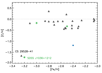
Figure 9: Abundance of carbon as a function of [Fe/H]. Abundances from literature are plotted as open triangles, while star symbols are from this work. The filled circle shows CS 22964-161.

The nitrogen abundances are shown in Fig. 10 as a function of [C/Fe]. While CS 29528-041 exhibits a high N abundance for its low C abundance, SDSS J1036+1212 displays a nitrogen abundance in the expected range, as do the other two stars in this work.

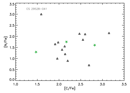
Figure 10: Abundance of nitrogen as a function of [C/Fe]. Abundances from literature are plotted as open triangles, while star symbols are from this work.

Our nitrogen abundances and lower limits on carbon isotopic ratios are compatible with the predictions of models of hot bottom burning in the envelopes of AGB stars (Karakas & Lattanzio, 2007). According to these authors intermediate-mass low-metallicity AGB stars produce low C/N and ¹²C/¹³C isotopic ratios, while low-mass AGB stars produce high C/N and ¹²C/¹³C isotopic ratios. We measured [C/N] = 1.22 for SDSS J1349-0229 and have a lower limit of 30 on its carbon isotopic ratio, qualitatively compatible with a low-mass AGB donor. We found a much lower value, [C/N] = 0.42, for SDSS J0912+0216, and a lower limit on the carbon isotopic ratio of 10, compatible with an intermediate-mass AGB donor.

5.3 Neutron-capture elements

The abundance ratio of barium, representative of the $s$-process, to europium (representative of the $r$-process) is plotted in Fig. 11 as a function of metallicity. For comparison we have also plotted [Ba/Eu] for the sample of extremely metal-poor stars from François et al. (2007). Here SDSS J1036+1212 separates itself again from the sample of CEMP-r/s stars, as the [Ba/Eu] ratio is more similar to that observed in EMP stars, where we expect a pure $r$-process origin for the neutron-capture elements.

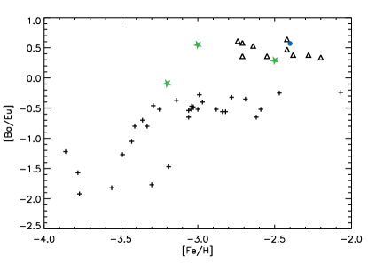
Figure 11: [Ba/Fe] as a function of [Eu/Fe]. Abundances from literature are plotted as open triangles, while star symbols are from this work. Included in this plot are EMP stars from François et al. (2007), plotted as crosses.

The [Ba/H] can be used as an indicator of the $s$-process efficiency of the donor AGB star. We have plotted [Sr/Ba] as a function of [Ba/H] for the sample of stars in Fig. 12. A clear anti-correlation is seen between [Sr/Ba] and [Ba/H] as well as a progression from the stars with less $s$-process efficiency (CEMP-no, EMP) to those with high efficiency (CEMP-r/s). The production ratio of heavy to light neutron-capture elements increases with total production efficiency.

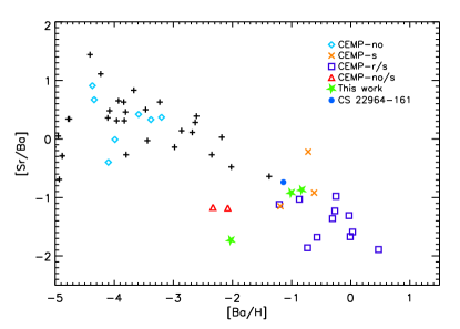
Figure 12: The Sr/Ba ratio of our sample of stars compared to the classes of stars listed in Table 8 and the sample of extremely metal-poor stars from François et al. (2007).

We compared the element distributions of our three stars to theoretical model surface compositions of AGB stars. We employed models from Cristallo et al. (2009a) and Cristallo et al. (2009b). The results are shown in Fig. 13, 14 and 15. The models were computed using the FRANEC code (Chieffi et al. 1998). The first model used in the comparison was computed with an initial mass of 2M_☉ and [Fe/H] = –2.14. The second has an initial mass of 1.5M_☉ and [Fe/H] = –2.44.

There is very little difference between the two models in the predicted distribution of the light elements, but larger C, N and O values are produced in the model with the lower mass and metallicity. The models diverge at Z $>$ 30; the heavier elements are on average 1.0 dex more abundant in the lower metallicity model compared to the high metallicity, high mass model.

In general, the light $s$ elements (Sr, Y, Zr, hereafter $ls$) of the three stars are better reproduced by the more massive AGB model, while the heavy $s$ elements (Ba to Hf, hereafter $hs$) are better reproduced by the less massive AGB model. We are however limited by the two models used in our comparison. Bisterzo & Gallino (2008) presented a comparison between a sample of 74 CEMP-s and CEMP-r/s stars and theoretical AGB models with different ¹³C-pocket efficiencies, initial masses (M= 1.3,1.5,2,3 M_☉), and metallicities (–3 $<$ [Fe/H] $<$ –1). Their results showed that the low [$ls$/Fe] values found in CEMP stars can best be reproduced at low metallicities with lower initial AGB masses ( M $<$ 1.4 M_☉). Additionally, a strong initial $r-$enrichment of the order of [$r$/Fe] = 2.0 dex was needed to match the observations of several CEMP-r/s stars.

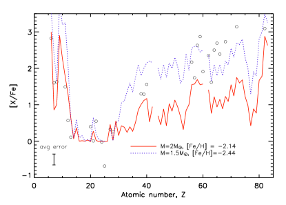
Figure 13: Element distribution of SDSS J1349-0229 compared to model surface abundances of AGB stars. The first model, shown in red, has an initial mass of 2 M_☉ and [Fe/H] = –2.14 (Cristallo et al. 2009). The second model has an initial mass of 1.5 M_☉ and [Fe/H] = –2.44 (Cristallo et al. 2009b).

Figure 14: As Fig. 13 for SDSS J0912+0216.

Figure 15: As Fig. 13 for SDSS J1036+1212.

6 Discussion and conclusions

We classify SDSS J1349-0229 and SDSS J0912+0216 as CEMP-r+s stars. SDSS J1349-0229 shows clear radial-velocity variations following two sets of observations, which indicates that it is a member of a binary system. SDSS J1036+1212 shows similarities with CS 29528-041, a CEMP-no/s star. They have similar temperatures, gravities and metallicities. They also both stand out as carbon-poor with respect other CEMP stars. They differ in their nitrogen and $s$ and $r$-process abundances however. The [$hs$/$ls$] ratio is higher for SDSS J1036+1212 compared to CS 29528-041, suggesting that the initial mass of the AGB companion star is lower for SDSS J1036+1212 than for CS 29528-041 (Bisterzo & Gallino 2008). An AGB star with a higher initial mass would produce less heavy neutron-capture elements (see Fig. 13, 14 and 15). We measured [Ba/Fe] = 1.17 in SDSS J1036+1212, while the observed value in CS 29528-041 is 0.97. Furthermore, CS 29528-041 is extremely enhanced in nitrogen: [N/Fe] = +3.07, while SDSS J1036+1212 is moderately enhanced with [N/Fe] = +1.29. High initial mass AGB models by Herwig (2004) with M $>$ 4M$\sun$ predict high nitrogen and low carbon, whereas the lower mass models predict lower nitrogen and high carbon. The high mass AGB models predict carbon abundances similar to those observed in these two stars. A plausible origin can therefore be determined for CS 29528-041 in pollution from a high mass AGB star. The elements observed in SDSS J1036+1212 point towards pollution by a low mass AGB companion. The low carbon abundance though is puzzling and cannot be explained by current models. Furthermore, the Li and [Ba/Eu] is similar to that observed in EMP stars.

The scenario of mass transfer from an AGB companion is certainly the one which allows the explanation of most of the chemical abundances observed in the three stars studied in this work. The high Li abundance observed in one of them poses some problems: if it is attributed to a production in the AGB star, it requires some very fine tuning between Li production and destruction. Finally it is somewhat surprising that all three stars show a large (over 1  dex) enhancement of Eu, which is a pure r-process element. This does not fit the AGB nucleosynthesis and requires another origin. As all three stars show this signature, it implies that such an event is relatively common among CEMP stars.