A Pedagogical “Toy” Bistable Climate Model

Abstract

A “toy” model, simple and elementary enough for an undergraduate class, of the temperature dependence of the greenhouse (mid-IR) absorption by atmospheric water vapor implies a bistable climate system. The stable states are glaciation and warm interglacials, while intermediate states are unstable. This is in qualitative accord with the paleoclimatic data. The present climate may be unstable, with or without anthropogenic interventions such as CO₂ emission, unless there is additional stabilizing feedback such as “geoengineering”.

I Introduction

Models of climate change, a subject that concerns time scales from decades to billions of years, range from the simple and qualitative to atmospheric and oceanic general circulation models running on the fastest computers. Despite several decades of effort by many scientists, the causes of such important phenomena as the alternation of glaciation and interglacials, and the ice ages themselves, remain controversial. In this pedagogical paper I describe an elementary and qualitative model of the consequences of one important effect, the temperature dependence of the opacity of atmospheric water vapor, the most important greenhouse gasKiehl and Trenberth (1997). This is a consequence of the temperature dependence of the water vapor pressure and the physics of pressure broadening of saturated Lorentzian spectral line profiles, and lies on the border between physics and geophysics.

II Paleoclimatic Data

The paleoclimatic data are summarized in Figure 1. Alternation of ice ages and interglacials is evident. Intermediate states, such as the present climate, are not stable or steady, but show continual variation. This is also evident in the historical record of the Late Medieval Climatic Maximum (c. 800–1300), followed by the Little Ice Age (c. 1300–1800), followed in turn by a warming trend.

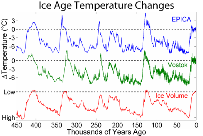
Figure 1: Paleoclimatic data showing ice ages and interglacialsW09 (Accessed Dec. 30, 2009); EPICA (2004); Petit et al. (1999); Lisiecki and Raymo (2005).

III Water Vapor Opacity

Although water vapor is the greatest source of atmospheric opacity in the mid-infrared (8–14 $\mu$) band in which the Earth’s thermal emission peaks, it is not even mentioned in a classic monographSaltzman (2002) on climatological dynamics. The HITRAN databaseRothman et al. (2009) is the comprehensive source of spectral information. Measurements of atmospheric opacity, such as those shown in Fig. 3 of Hiriart and SalasHiriart and Salas (2007), illustrate its sensitivity to even small amounts of water vapor.

Tropospheric water vapor is not usually considered in the context of anthropogenic greenhouse gas (GHG) emissions because it equilibrates with surface water very rapidly, with a characteristic time of a few days or less, and any anthropogenic contribution has no long term effect. Tropospheric water vapor opacity is controlled by evaporation and precipitation to a level determined by the surface temperature.

IV Limit States

This sensitivity of opacity to water vapor pressure, combined with the sensitivity of equilibrium vapor pressures to temperature, qualitatively suggests a bistable system: There may be a cold state in which the water precipitates and the atmosphere is transparent, with little water vapor absorption, and a warm state in which the atmosphere is warm, humid and opaque and in which absorbed solar energy is carried through the troposphere by convection (resembling present tropical or temperate summer conditions).

These limit states are stable: in the cold state perturbations to the temperature have little effect on the infrared opacity because it remains very low, while in the warm state the opacity has little effect on the heat transfer. In either case there is little feedback to the heat balance from changes in the tropospheric water vapor content. At intermediate temperatures increases in temperature produce a positive feedback by increasing the infrared opacity (and vice versa for decreases), so that perturbations grow exponentially until one of the stable limit states is approached.

V Model

Quantitative calculation is precluded by the complexity of the climate system. These complexities includ processes that are difficult to calculate but understood in principle (such as opacity resulting from a dense comb of infrared vibration-rotation lines) and those not understood (such as cloud formation and greenhouse gas exchange with the ocean, soil and biosphere). Even the most elaborate and sophisticated general circulation models (GCM) contain many uncertain parameters that can only be calibrated at a single measured point: today’s climate. It is not surprising that different GCM disagree in the magnitude of the effect of GHG emission, and it is not evident how to resolve these disagreements.

Disagreements among the best state-of-the-art GCM suggest considering the opposite approach, a model naïve almost to the point of triviality. If its workings are transparent, it may provide useful insight, even though it cannot make quantitative predictions.

Consider a surface heat reservoir warmed by sunlight with a mean (diurnally and annually averaged) intensity $P_{\odot}$ and cooled by black body radiative emission with a (Planck weighted) fraction $f_{b}(T)$ of the infrared spectrum blocked by lines of Lorentzian lineshapeGoody (1964) (Doppler broadening of molecular lines is negligible at atmospheric temperatures). The optical depth at the centers of strong lines $\tau_{0}\gg 1$, and assume an underlying heat capacity (per unit area) $C_{p}$. The temperature $T$ of the thermal reservoir changes at a rate

$$C_{p}{dT\over dt}=P_{\odot}-\sigma_{SB}T^{4}\left(1-f_{b}(T)\right),$$ (1)

where $\sigma_{SB}$ is the Stefan-Boltzmann constant and we approximate the line profile as completely opaque within a blocked fraction $f_{b}(T)$ of the spectrum, and completely transparent outside it.

We suppose an initial equilibrium temperature $T_{0}$ defined by the heat balance condition:

$$0=P_{\odot}-\sigma_{SB}T_{0}^{4}\left(1-f_{b}(T_{0})\right).$$ (2)

Small deviations of temperature are described by

$$T=T_{0}+\delta T.$$ (3)

VI Instability

Expanding Eq. 1 to first order in $\delta T$:

$${1\over\nu_{0}T_{0}}{d\delta T\over dt}\approx\left[{df_{b}(T)\over dT}-{4\over T_{0}}\left(1-f_{b}(T_{0})\right)\right]\delta T,$$ (4)

where

$$\nu_{0}\equiv{\sigma_{SB}T_{0}^{3}\over C_{p}}.$$ (5)

$\delta T$ grows or decays with an exponentiation rate $\nu$:

$${\nu\over\nu_{0}}=T_{0}{df_{b}(T)\over dT}-4\left(1-f_{b}(T_{0})\right).$$ (6)

To estimate the derivative in Eq. 6 we use an approximate equation Reif (1965) for the saturation water vapor pressure over a surface of temperature $T$:

$$p_{v}(T)\propto T^{3/2}\exp{(-\Delta H/k_{B}T)},$$ (7)

where $\Delta H=2260$ J/g is the enthalpy of evaporation of water and $k_{B}$ is Boltzmann’s constant. For a Lorentzian line profile with $\tau_{0}\gg 1$, the width and $f_{b}$ at a specified optical depth ${\cal O}(1)$

$$f_{b}(T)\approx f_{b}(T_{0})\left({\tau_{0}(T)\over\tau_{0}(T_{0})}\right)^{1/2}\approx f_{b}(T_{0})\left({p_{v}(T)\over p_{v}(T_{0})}\right)^{1/2}.$$ (8)

Then

$$\left.{df_{b}(T)\over dT}\right|_{T_{0}}={1\over T_{0}}f_{b}(T_{0})\left({\Delta H\over 2k_{B}T_{0}}+{3\over 4}\right)$$ (9)

and

$${\nu\over\nu_{0}}=f_{b}(T_{0})\left[{\Delta H\over 2k_{B}T_{0}}+{3\over 4}-4\left(1-f_{b}(T_{0})\right)\right],$$ (10)

where we have made the tacit assumptions $1-f_{b}(T_{0})>\tau_{0}^{-1/2}$, which amount to assuming that there is enough unblocked spectrum for the line to broaden according to Eq. 8. The appropriate value of $\tau_{0}$ in this condition is an average over all lines that are optically thick at their cores. This is likely to be dominated by the very numerous lines for which $\tau_{0}$ exceeds unity by a factor of a few, but not by orders of magnitude, so these results may be valid for $f_{b}\lesssim 0.7$. The model breaks down as $f_{b}\to 1$ because then there is little unblocked spectrum into which the lines can broaden.

Evaluating at a sea surface $T_{0}=290^{\,\circ}$K,

$${\nu\over\nu_{0}}=13.2f_{b}(T_{0})-4.$$ (11)

A quantitative calculation of $f_{b}$ is not possible within this qualitative model, but spectral dataHiriart and Salas (2007) suggest values of several tenths. Then deviations from equilibrium grow exponentially for

$$0.3<f_{b}\lesssim 0.7.$$ (12)

The mean ocean depth, averaged over the entire Earth (including zero depth for land areas) is about 2.65 km. However, the flow of heat to the deep ocean, while apparently reflecting the warming of the last century Dushaw et al. (2009), is expected to be confined to downwelling regions and to be comparatively slow. For the purpose of an order of magnitude estimate we suppose a nominal mean depth of 1 km contributes to $C_{p}$ and find

$$\nu_{0}=1.04\times 10^{-2}/{\rm y}.$$ (13)

VII Conclusion

If $0.3<f_{b}\lesssim 0.7$, as suggested by the empirical water vapor spectrumHiriart and Salas (2007), then instability would be expected for any state between an ice age (when $p_{v}$ is low enough that the assumption $\tau_{0}\gg 1$ is not satisfied) and the warmest interglacials (when the assumption $1-f_{b}(T_{0})>\tau_{0}^{-1/2}$ is not satisfied as nearly the entire thermal infrared spectrum is blanketed with water lines and $f_{b}\to 1$, or energy is carried by convection, ignored in this naïve model). Hence the climate would be stable only in these two limiting states.

The paleoclimatic data, as shown in Figure 1, are qualitatively consistent with this model. The historic record of the Medieval Climatic Maximum, the Little Ice Age, and fluctuations on similar time scales of ${\cal O}(100)$ years at other epochs, is also qualitatively consistent with the estimated $\nu_{0}$.

VIII Discussion

Climatologists have struggled with the question of what upsets the stable ice age and interglacial states since the discovery of the ice ages, and this naïve model cannot contribute to its answer. Even the most complete and sophisticated general circulation models struggle with this problem, and its resolution remains controversial. However, even the conclusion that intermediate states may be intrinsically unstable has significant implications. One implication is that there is no “normal” climate, nor can the Earth be expected to return to such a state even without anthropogenic interventions such as the emission of GHG. A second implication is that if some climate state is determined to be optimal for humanity, maintaining it would require continual active intervention (geoengineering).