Simplified model for the energy levels of quantum rings in single layer and bilayer graphene

Abstract

Within a minimal model, we present analytical expressions for the eigenstates and eigenvalues of carriers confined in quantum rings in monolayer and bilayer graphene. The calculations were performed in the context of the continuum model, by solving the Dirac equation for a zero width ring geometry, i.e. by freezing out the carrier radial motion. We include the effect of an external magnetic field and show the appearance of Aharonov-Bohm oscillations and of a non-zero gap in the spectrum. Our minimal model gives insight in the energy spectrum of graphene-based quantum rings and models different aspects of finite width rings.

I Introduction

The investigation of low-dimensional solid state devices has allowed the direct observation of quantum behavior in electron systems. These effects arise due to the confinement of carriers in structures that constrain their movement along one or more directions, such as quantum wells, quantum wires and quantum dots. One important class of such low-dimensional systems are quantum rings, in which a particular type of confinement together with phase coherence of the electron wavefunction allows the observation of effects such as the Aharonov-Bohm AB and Aharonov-Casher AC effects. Quantum rings have been extensively studied in semiconductor systems, both experimentally and theoretically Bichier and are expected to find application in microelectronics, as well as in future quantum information devices.

In this paper we present analytical results for the eigenstates and energy levels of ideal quantum rings created with graphene and bilayer graphene. Graphene is an atomic layer of crystal carbon which has been the target of intense scrutiny since it has been experimentally produced novo3 ; novo4 ; shara ; zhang . Part of this interest stems from the unusual properties of carriers in graphene, caused by the gapless and approximately linear carrier spectrum, together with possible technological applications, such as transistors, gas sensors and transparent conducting materials in e.g. photovoltaics. Additionally, it has been found that two coupled graphene sheets, also known as bilayer graphene displays properties that are distinct from single layer graphene as well as from graphite. The carrier spectrum of bilayer graphene is gapless and approximately parabolic at the vicinity of two points in the Brillouin zone Bart ; Ohta . In particular, the spectrum is strongly influenced by an external electric field perpendicular to the bilayer, leading to the appearance of a gap McCann . The high quality of the single layer and bilayer graphene samples that have been obtained, together with the large mean free path of carriers suggests that phase coherence effects may be observable in these systems. Recently, graphene-based quantum rings produced by lithographic techniques have been investigated on single-layer graphene Russo ; Molitor . These systems have been studied theoretically by means of a tight-binding model, which does not provide straightforward analytical solutions for the eigenstates and eigenvalues Recher ; Wurm ; Luo ; Rycerz ; Bahamon . For bilayer graphene also it was recently shown Zarenia that is possible to electrostatically confine quantum rings with a finite width. The energy spectrum was obtained by solving the Dirac equation numerically.

In this paper we present a toy model that allows for analytical expressions for the energy levels of quantum rings in single layer and bilayer graphene. This model permits the description of several aspects of the physics of graphene quantum rings without the additional complications of edge effects and finite width of the quantum ring. We are able to obtain analytical expressions for the energy spectrum and the corresponding wavefunctions, the persistent current, and the orbital momentum as function of ring radius, total momentum and magnetic field, which can be related to the numerical results obtained by other methods.

The paper is organized as follows: in section II we present the theoretical model and numerical results for quantum rings in single layer graphene. Similar results for bilayer graphene are given in Sect. III. Section IV contains a summary of the main results and the conclusions.

II Single layer graphene

II.1 Model

The dynamics of carriers in the honeycomb lattice of covalent-bond carbon atoms of single layer graphene can be described by the Dirac Hamiltonian (valid for $E<0.8$ eV). In the presence of a uniform magnetic field ${\mathbf{B}}=B_{0}{\mathbf{e}}_{z}$ perpendicular to the plane and finite mass term $\Delta$, which might be caused by an interaction with the underlaying substrate McCann ; Recher2 The Hamiltonian in the valley isotropic form is given by Recher :

$$H=v_{F}(\mathbf{p}+e\mathbf{A}).\boldsymbol{\sigma}+\tau\Delta\sigma_{z}$$ (1)

where $\tau=+1$ corresponds to the $K$ point and $\tau=-1$ to the $K^{\prime}$ point. ${\mathbf{p}}$ is the in-plane momentum operator, $\mathbf{A}$ is the vector potential and $v_{F}\approx 1.0\times 10^{6}$ m$/$s is the Fermi velocity, and $\boldsymbol{\sigma}=(\sigma_{x},\sigma_{y},\sigma_{z})$ is the pseudospin operator with components given by Pauli matrices. The eigenstates of Eq. (1) are two-component spinors which, in polar coordinates is given by

$$\Psi(\rho,\phi)=\left(\begin{array}[]{c}\phi_{A}(\rho)e^{im\phi}\\ i\phi_{B}(\rho)e^{i(m+1)\phi}\\ \end{array}\right).$$ (2)

where $m$ is the angular momentum label. We follow the earlier very successful approach Meijer ; Molnar of ideal one-dimensional (1D) quantum rings in semiconductors with spin-orbit interaction where the Schrödinger equation was simplified by discarding the radial variation of the electron wave function. Thus, in the case of an ideal ring with radius $R$, the momentum of the carriers in the radial direction is zero. We treat the radial parts of the spinors in Eq. (2) as a constant

$$\Psi(R,\phi)=\left(\begin{array}[]{c}\phi_{A}(R)e^{im\phi}\\ i\phi_{B}(R)e^{i(m+1)\phi}\\ \end{array}\right).$$ (3)

Because the radial motion is frozen in our model there will be no radial current and the persistent current will be purely in the angular direction. By solving $H\Psi(R,\phi)=E\Psi(R,\phi)$ and using the symmetric gauge ${\bf A}=(0,B_{0}\rho/2,0)$, we obtain

$$(m+1+\beta)\phi_{B}(R)=(\epsilon-\tau\delta)\phi_{A}(R),$$ (4)

(5)

$$(m+\beta)\phi_{A}(R)=(\epsilon+\tau\delta)\phi_{B}(R),$$ (6)

where the energy and mass terms are written in dimensionless units as $\epsilon=E/E_{0}$, $\delta=\Delta/E_{0}$ with $E_{0}=\hbar v_{F}/R$. The parameter $\beta=(eB_{0}/2\hbar)R^{2}$ can be expressed as $\beta=\Phi/\Phi_{0}$ with $\Phi=\pi R^{2}B_{0}$ being the magnetic flux threading the ring and $\Phi_{0}=h/e$ the quantum of magnetic flux. The homogeneous set of equations (4) is solvable for the energies

$$\epsilon=\pm\sqrt{(m+\beta+1)(m+\beta)+\delta^{2}}.$$ (7)

This energy can also be written as

$$\epsilon=\pm\sqrt{(m-m_{-})(m-m_{+})}$$ (8)

where

$${m_{\pm}=-(\beta+\frac{1}{2})\pm\sqrt{\frac{1}{4}-\delta^{2}}}.$$ (9)

Note that the energy spectrum for an ideal single layer quantum ring for both $K$ and $K^{\prime}$ points are the same. For $|\delta|>1/2$ we have that $m_{+}=m_{-}^{*}$ is complex and $\epsilon$ is real for any value of $\beta$. In the region $-\frac{1}{2}<\delta<\frac{1}{2}$ the energy is real, except for $m_{-}<m<m_{+}$, when the energy is complex. For the gapless case, i.e. $\delta=0$, we have $m_{+}=-\beta$ and $m_{-}=-\beta-1$ and the energy is real when $m<-\beta-1$ or when $m>-\beta$ and imaginary otherwise.

The wavefunctions are eigenfunctions of the total angular momentum operator given by the sum of orbital angular momentum $L_{z}$ and a term describing the pseudo-spin $S_{z}$

$$J_{z}=L_{z}+\hbar S_{z},$$ (10)

where $S_{z}=(1/2)\sigma_{z}$, with $\sigma_{z}$ being one of the Pauli matrices and the eigenvalues of $J_{z}$ operator become $[m+(1/2)]\hbar$.

The current is obtained using $j_{x,y}=v_{F}[\psi^{\dagger}\sigma_{x,y}\psi]$. The total angular current $j=v_{F}[\psi^{\dagger}\sigma_{\phi}\psi]$ can be calculated using the fact that $\sigma_{\phi}=\xi(\phi)\sigma_{y}$, where

$$\xi(\phi)=\begin{pmatrix}e^{-i\phi}&0\\ 0&e^{i\phi}\end{pmatrix}.$$ (11)

The current for the electrons in the K-valley becomes

$$j_{K}=v_{F}(\phi_{A}^{*}\phi_{B}+\phi_{B}^{*}\phi_{A}).$$ (12)

The total current is then given by $j=j_{K}+j_{K^{\prime}}$. The radial part of the two spinor components are

$$\phi_{A}(R)=1,\quad\phi_{B}(R)=\frac{m+\beta}{\epsilon+\tau\delta}.$$ (13)

Notice that the radial current can be calculated using $j_{r}=v_{F}[\psi^{\dagger}\xi(\phi)\sigma_{x}\psi]$ which leads to the the following relation,

$$j_{r}=iv_{F}(\phi_{A}^{*}\phi_{B}-\phi_{B}^{*}\phi_{A}),$$ (14)

where, in the case of our ideal ring we have $j_{r}=0$. From Eqs. (12) and (13), one can find the following expression for the total angular current of a single layer quantum ring

$$j=\frac{4v_{F}\epsilon(m+\beta)}{\epsilon^{2}-\delta^{2}}.$$ (15)

One can rewrite Eq. (15) in the following form

$$\frac{j}{v_{F}}=\big{(}\frac{\partial\epsilon}{\partial\beta}\big{)}_{K}+\big{(}\frac{\partial\epsilon}{\partial\beta}\big{)}_{K^{\prime}}+\frac{2(m+\beta)(\epsilon^{2}+\delta^{2})-(\epsilon^{2}-\delta^{2})}{\epsilon(\epsilon^{2}-\delta^{2})}.$$ (16)

Since for the ground state energy $\sqrt{\delta^{2}-1/4}\leq\epsilon\leq\delta$ and $-1/2\leq m+\beta\leq 0$ the last term in Eq. (13) is much smaller than the derivatives of the energy with respect to the flux ($\Phi$) and oscillates around zero. Note that in 1D semiconductor rings the current is exactly given by $\partial E/\partial\Phi$, which is thus different from graphene where we have approximately

$$\frac{j}{v_{F}}\simeq\big{(}\frac{\partial\epsilon}{\partial\beta}\big{)}_{K}+\big{(}\frac{\partial\epsilon}{\partial\beta}\big{)}_{K^{\prime}}.$$ (17)

with $\beta=\Phi/\Phi_{0}$.

II.2 Results

The energies as function of ring radius R are shown in Fig. 1, for $\Delta=50$ meV, with $-10\leq m\leq-1$ (magenta curves), $1\leq m\leq 10$ (blue curves), and $m=0$ (green curves). In the absence of an external magnetic field, the energy is given by $E=\pm\sqrt{m(m+1)(\hbar v_{F}/R)^{2}+\Delta^{2}}$ and the energy branches have a $1/R$ dependence and approach $E\rightarrow\pm\Delta$ for very large radii. Note that for $m=0$ and $m=-1$ the energy $E=\pm\Delta$ is independent of $R$ and all branches are two-fold degenerate. For non-zero magnetic field ($B=3$T), the right panel shows that the branches have an approximately linear dependence on the ring radius for large $R$, in particular we have $E\simeq\pm\sqrt{(\alpha R)^{2}+\Delta^{2}}$, with $\alpha=v_{F}eB_{0}/2$. For small radii, $E\simeq\pm\hbar\sqrt{m(m+1)}/R$ and all branches diverge as $1/R$, except for $m=0$ and $m=-1$. In those cases when $R\rightarrow 0$ we have for $m=0$ the result $E=\pm\sqrt{\Delta^{2}+\alpha\hbar v_{F}}$, while $m=-1$ gives $E=\pm\sqrt{\Delta^{2}-\alpha\hbar v_{F}}$.

Figure 2 presents results for the energy as function of total angular momentum index $m$, for $\Delta=50$ meV, $R=50$ nm and for three different values of magnetic field, namely $B_{0}=-5$ T (diamonds), $B_{0}=0$ T (circles) and $B_{0}=5$ T (triangles). Notice that for a given $B_{0}$ the electron energy obtains a minimum for a particular $m$, i.e. for $B_{0}=0$ ($5$ T, $-5$ T) it is $m=0$ ($9$, $-10$). In fact it is given by $m=-(\Phi/\Phi_{0}+1/2)$ and is independent of $\Delta$.

The energy levels as function of the external magnetic field are shown in Fig. 3, for a quantum ring with (a) $\delta=1/2$, (b) $\delta=3/8$, (c) $\delta=1/4$ and (d) $\delta=0$ with $R=50~{}nm$ for $-10\leq m\leq-1$ (red curves), $1\leq m\leq 10$ (blue curves), and $m=0$ (green curves). The magnetic field dependence of the spectrum becomes evident if one rewrites Eq. (5) as $\epsilon^{2}-[(m+\Phi/\Phi_{0})+1/2]^{2}=\delta^{2}-1/4$. Thus, for the special case of $\delta=\Delta/E_{0}=1/2$ the gap is zero and the energy levels are straight lines given by $\epsilon=\pm(m+1/2+\Phi/\Phi_{0})$. The energy spectra for $\delta>1/2$ resemble those found earlier by Recher et al. Recher in the case of a finite width graphene ring with infinite mass boundary conditions. An enlargement of Fig. 3 around $E=0$ is shown in Fig. 4. The spectrum has an interesting magnetic field dependence with decreasing $\delta$. For $\delta=0$ the double degeneracy is restored at $E=0$. This behavior can be easily illustrated by considering $m=0$. The energy in this case is $\epsilon=\pm\sqrt{\beta(\beta+1)+\delta^{2}}$ which for $\delta=1/2$ becomes $\epsilon=\pm(\beta+1/2)$ while for $\delta=0$ it is $\epsilon=\pm\sqrt{\beta(\beta+1)}$ and thus $\epsilon\simeq\pm\sqrt{\beta}$ for $\beta\simeq 0$.

In Fig. 5(a) the energy spectrum is plotted vs magnetic field for $\delta=2$. Where, the energy has a hyperbolic dependence on the applied magnetic field with minima at $\Phi/\Phi_{0}=-m-1/2$ and a gap of $\Delta\epsilon=2\sqrt{\delta^{2}-1/4}$. The exact location of the transitions (orange dots) and the location of the minima points (yellow dots) in the energy spectrum is clarified in Fig. 5(b). The dependence of the energy levels on the gap parameter $\Delta$ is shown in Fig. 6, for zero magnetic field (left panels) and $B_{0}=1$ T (right panels). When $m\geq 0$ (upper panels) and $m<0$ (lower panels). For $B_{0}=0$ T the energy levels are two fold degenerate where $E(m)=-E(-m-1)$. When a magnetic field is applied an energy gap is opened (see right-bottom panel in Fig. 6). Notice also that the $m=-2$ level only exists for $\Delta\geq E_{0}/2$, i. e. for $\Delta<E_{0}/2$ there is no real energy solution when $m=-2$.

The corresponding ground state expectation values for the operators in Eq. (8) are plotted as function of the magnetic field in Fig. 7(b) for both $K$ (black dashed curve) and $K^{\prime}$ valley (black dash-dotted curve). Notice that for the $K$-valley $<L_{z}>\simeq m\hbar$ and $<S_{z}>\simeq\hbar/2$ whereas in the $K^{\prime}$-valley $<L_{z}>\simeq(m+1)\hbar$ and $<S_{z}>\simeq-\hbar/2$. Thus for both the $K$ valley and the $K^{\prime}$ valley $<J_{z}>\simeq[m+(1/2)]\hbar$ which is approximately quantized and on the average its value decreases linearly with the applied magnetic field.

The angular current density for a single layer graphene quantum ring is shown in Fig. 8(c). Note that the contribution from the $K$-valley $j_{K}$ (Fig. 8(a)) and the $K^{\prime}$-valley $j_{K^{\prime}}$ (Fig. 8(b)) are not the same, they have opposite sign and oscillate in phase around a nonzero average value $-\tau v_{F}/4$. The reason is that if for given energy we have electrons in the $K$-valley, the corresponding particles in the $K^{\prime}$-valley will behave as holes. The persistent current is a sawtooth shaped oscillating function of the magnetic field with period $\Delta B_{0}=\Phi_{0}/\pi R^{2}$. This behavior is quantitatively very similar to those found for the standard Aharanov-Bohm oscillations in metallic and semiconductor quantum rings.

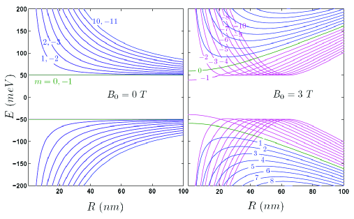
Figure 1: (Color online) Energy levels with $m=-10,...,10$ of single layer graphene quantum ring as function of ring radius $R$ for $B_{0}=0$ T (left panel) and $B_{0}=3$ T (right panel) when the mass term is $\Delta=50$ meV.

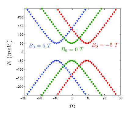
Figure 2: (Color online) Energy levels of a single layer graphene quantum ring as function of the quantum number $m$ for $B_{0}=-5,0,5$ T with $\Delta=50$ meV and $R=50$ nm.

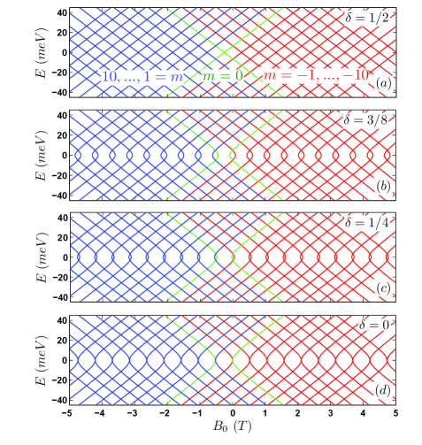
Figure 3: (Color online) Electron and hole energy levels of a single layer graphene quantum ring as function of external magnetic field $B_{0}$ for (a) $\delta=1/2$, (b) $\delta=3/8$, (c) $\delta=1/4$ and (d) $\delta=0$ with $R=50$ nm, and total angular quantum number $-10\leq m\leq-1$ (red curves), $1\leq m\leq 10$ (blue curves) and $m=0$ (green curves).

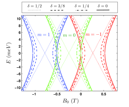
Figure 4: (Color online) The same as Fig. 3, for $m=-1$ (red curves), $m=1$ (blue curves) and $m=0$ (green curves) and different values of dimensionless mass term $\delta$.

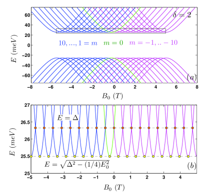
Figure 5: (Color online) (a) Electron and hole energy levels of a single layer graphene quantum ring as function of external magnetic field $B_{0}$ for $\delta=2$ and $R=50$ nm. (b) An Enlargement of the region which is shown in (a) by a rectangle.

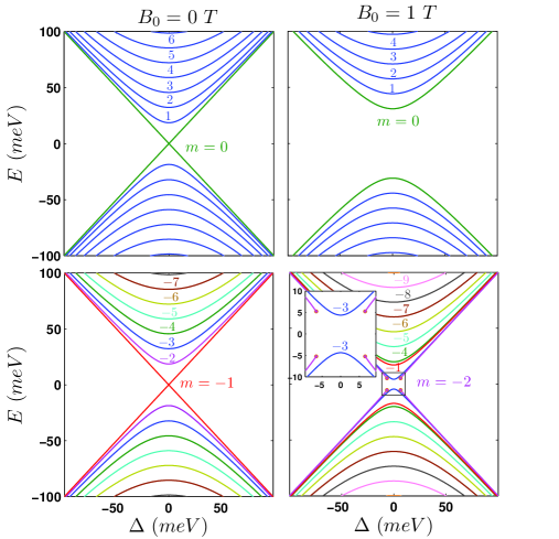
Figure 6: (Color online) Lowest energy levels of a single layer graphene quantum ring as function of the mass term $\Delta$ with $B_{0}=0$ T (left panels) and $B_{0}=1$ T (right panels) for $m\geq 0$ (upper panels) and $m<0$ (lower panels) with $R=50$ nm.

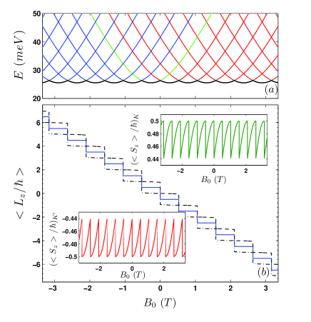
Figure 7: (Color online) (a) Electron energy levels of a graphene single layer quantum ring as function of external magnetic field $B_{0}$ for the same parameters as used in Fig. 5. Black curve shows the ground state energy (b) Ground state expectation value of $L_{z}/\hbar$ as function of magnetic field for both $K$ (black dashed curve) and $K^{\prime}$ valley (black dash-dotted curve). Expectation value of $S_{z}/\hbar$ versus magnetic field is plotted in upper inset for $K$-valley and in lower inset for $K^{\prime}$-valley. Blue solid curve shows the expectation value $<J_{z}>$ which is the same for both valleyes.

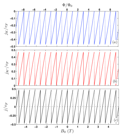
Figure 8: The angular current density in the (a) $K$-valley, (b) $K^{\prime}$-valley and (c) the total current density of a monolayer graphene quantum ring as function of external magnetic field $B_{0}$ for the ground state energy shown by the black curve in Fig. 7(a).

III Bilayer graphene

III.1 Model

In the case of bilayer graphene the Hamiltonian in the vicinity of the $K$ point, is given byMcCann

$$H=\left(\begin{array}[]{cccc}\tau U_{1}&\pi&t&0\\ \pi^{{\dagger}}&\tau U_{1}&0&0\\ t&0&\tau U_{2}&\pi^{{\dagger}}\\ 0&0&\pi&\tau U_{2}\\ \end{array}\right)$$ (18)

where $\tau=\pm 1$ distinguishes the two $K$ and $K^{\prime}$ valleys. $t\simeq 400$ meV is the interlayer coupling term, $\pi=v_{F}[(p_{x}+eA_{x})+i(p_{y}+eA_{y})]$, $U_{1}$ and $U_{2}$ are the potentials, respectively, at the two graphene layers. Here we do not include any mass term because the gate potential across the bilayer is able to open an energy gap in the spectrum. McCann The eigenstates of the Hamiltonian (18), are four-component spinors $\Psi(r,\phi)=[\phi_{A}(\rho)e^{im\phi}\,,\,i\phi_{B}(\rho)e^{i(m-1)\phi}\,,\,\phi_{C}(\rho)e^{im\phi}\,,\,i\phi_{D}(\rho)e^{i(m+1)\phi}]^{T}$ (see Ref. [Milton, ]). Following our earlier approach for an ideal ring with radius $R$, the wave function becomes:

$$\Psi=\left(\begin{array}[]{c}\phi_{A}(R)e^{im\phi}\\ i\phi_{B}(R)e^{i(m-1)\phi}\\ \phi_{C}(R)e^{im\phi}\\ i\phi_{D}(R)e^{i(m+1)\phi}\\ \end{array}\right).$$ (19)

We use the symmetric gauge and obtain the following set of coupled algebraic equations

$$-(\epsilon-\tau u_{1})\phi_{A}(R)-(m+\beta-1)\phi_{B}(R)+t^{\prime}\phi_{C}(R)=0,$$ (20)

(21)

$$(m+\beta)\phi_{A}(R)+(\epsilon-\tau u_{1})\phi_{B}(R)=0,$$ (22)

(23)

$$t^{\prime}\phi_{A}(R)-(\epsilon-\tau u_{2})\phi_{C}(R)+(m+\beta+1)\phi_{D}(R)=0,$$ (24)

(25)

$$(m+\beta)\phi_{C}(R)-(\epsilon-\tau u_{2})\phi_{D}(R)=0.$$ (26)

where, $t^{\prime}=t/E_{0}$ and $u_{1,2}=U_{1,2}/E_{0}$ are in dimensionless units. After some straightforward algebra we obtain the following polynomial equation that determines the energy spectrum

$$(\epsilon-\tau u_{1})^{2}\bigr{[}(\epsilon-\tau u_{2})^{2}-(m+\beta)(m+\beta+1)\bigl{]}$$ (31)

$$-(m+\beta)(m+\beta-1)\bigr{[}(\epsilon-\tau u_{2})^{2}-(m+\beta)(m+\beta+1)\bigl{]}$$

$$-(\epsilon-\tau u_{1})(\epsilon-\tau u_{2})t^{\prime 2}=0.$$

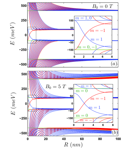
Figure 9: (Color online) Lowest energy levels of a bilayer graphene quantum ring as function of ring radius $R$ with (a) $B_{0}=0$ T and (b) $B_{0}=5$ T for $U_{b}=100$ meV and total angular quantum number $-10\leq m\leq-1$ (red curves), $1\leq m\leq 10$ (blue curves) and $m=0$ (green curves). The insets are an enlargement of the small energy and small $R$ region.

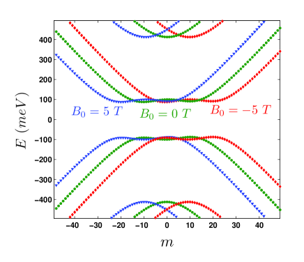
Figure 10: (Color online) Lowest energy levels of a graphene bilayer quantum ring as function of total angular momentum label $m$ for $B_{0}=-5,0,5$ T with $U_{b}=100$ meV and $R=50$ nm.

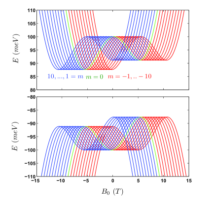
Figure 11: (Color online) Electron and hole energy states of a graphene bilayer quantum ring as function of external magnetic field $B_{0}$ for $U_{b}=100$ meV and $R=50$ nm. The energy levels are shown for the quantum numbers $-10\leq m\leq-1$ (red curves), $1\leq m\leq 10$ (blue curves) and $m=0$ (green curves).

After introducing the average potential $u=(u_{1}+u_{2})/2$ and half the potential difference $\delta=(u_{1}-u_{2})/2$ we can rewrite this quartic algebraic equation in a more comprehensive form:

$$s^{4}-2s^{2}[(m+\beta)^{2}+\delta^{2}+(t^{\prime})^{2}/2]$$ (32)

(33)

$$+4s\tau\delta(m+\beta)+(m+\beta)^{2}[(m+\beta)^{2}-1]$$ (34)

(35)

$$-2\delta^{2}[(m+\beta)^{2}-(t^{\prime})^{2}/2]+\delta^{4}=0,$$ (36)

where $s=\epsilon-\tau u$ is the energy shifted by the average potential. In the next section we report the results for the case of $U_{1}=-U_{2}=U_{b}$ where, the average potential $u$ is zero. In the limit $\delta\rightarrow 0$, the quartic equation is reduced to a quadratic equation in $s^{2}$ and we obtain the real solutions

$$s_{\pm}^{2} = (m+\beta)^{2}+(t^{\prime})^{2}/2$$ (39)

$$\pm\sqrt{(t^{\prime})^{4}/4+(m+\beta)^{2}(1+t^{\prime})^{2}},$$

which results in four solutions for the energy. These are real when $|m+\beta|\geq 1$. In the opposite case of $|m+\beta|<1$ (or equivalently $-1+\beta<m<1-\beta$) we have $s_{-}^{2}<0$ and consequently the corresponding energies are imaginary. In the limit of $t^{\prime}>>m+\beta$ we obtain $s_{-}^{2}=(m+\beta)^{2}[(m+\beta)^{2}-1]/(t^{\prime})^{2}$ and thus the low energy solutions are given by

$$s\simeq\pm\frac{1}{t^{\prime}}\sqrt{(m+\beta)^{2}((m+\beta)^{2}-1)}.$$ (40)

For bilayer graphene, the wavefunctions are eigenfunctions of the following operator:

$$J_{z}=L_{z}+\hbar\tau_{z}+\hbar S_{z},$$ (41)

where now

$$\tau_{z}=\frac{1}{2}\begin{pmatrix}-{\mathbf{I}}&0\\ 0&{\mathbf{I}}\end{pmatrix}\quad,\quad S_{z}=\frac{1}{2}\begin{pmatrix}\sigma_{z}&0\\ 0&-\sigma_{z}\end{pmatrix},$$ (42)

are $4\times 4$ matrices.

In bilayer graphene the components of the current density are given by

$$j_{x}=v_{F}\left[\psi^{{\dagger}}\begin{pmatrix}{\sigma_{x}}&0\\ 0&{\sigma_{x}}\end{pmatrix}\psi\right]\quad,\quad j_{y}=v_{F}\left[\psi^{{\dagger}}\begin{pmatrix}-\sigma_{y}&0\\ 0&\sigma_{y}\end{pmatrix}\psi\right].$$ (43)

The angular current can be calculated from the following relation,

$$j=v_{F}\left[\psi^{{\dagger}}\begin{pmatrix}\sigma_{y}^{\ast}\xi(\phi)&0\\ 0&\xi(\phi)\sigma_{y}\end{pmatrix}\psi\right].$$ (44)

Where, $\xi(\phi)$ is given by Eq. (11). We obtain for the angular current in the K-valley,

$$j_{K}=v_{F}(\phi_{C}^{*}\phi_{D}+\phi_{D}^{*}\phi_{C}-\phi_{A}^{*}\phi_{B}-\phi_{B}^{*}\phi_{A}),$$ (45)

and the total angular current is given by $j=j_{K}+j_{K^{\prime}}$. Where, the four spinor components are:

$$\phi_{A}(R)=1,$$ (46)

(47)

$$\phi_{B}(R)=-\frac{m+\beta}{\epsilon-\tau u_{1}},$$ (48)

(49)

$$\phi_{C}(R)=\frac{(\epsilon-\tau u_{1})^{2}-(m+\beta)(m+\beta-1)}{t^{\prime}(\epsilon-\tau u_{1})},$$ (50)

(51)

$$\phi_{D}(R)=\frac{(m+\beta)[(\epsilon-\tau u_{1})^{2}-(m+\beta)(m+\beta-1)]}{t^{\prime}(\epsilon-\tau u_{1})(\epsilon-\tau u_{2})}.$$ (52)

(53)

Note that the radial current can be calculated through

$$j_{r}=v_{F}\left[\psi^{{\dagger}}\begin{pmatrix}\sigma_{x}\xi(\phi)&0\\ 0&\xi(\phi)\sigma_{x}\end{pmatrix}\psi\right],$$ (55)

where, $j_{r}=iv_{F}(\phi_{A}^{*}\phi_{B}-\phi_{B}^{*}\phi_{A}+\phi_{C}^{*}\phi_{D}-\phi_{D}^{*}\phi_{C})=0$ for the case of an ideal ring. Using Eq. (45), the total current density becomes,

$$j=\sum_{\tau=\pm 1}$$ (56)

(57)

$$\frac{2v_{F}(m+\beta)}{\epsilon-\tau u_{1}}\left[1+\frac{\big{[}(\epsilon-\tau u_{1})^{2}-(m+\beta)(m+\beta-1)\big{]}^{2}}{t^{\prime 2}(\epsilon-\tau u_{1})(\epsilon-\tau u_{2})}\right].$$ (58)

III.2 Results

The dependence of the spectrum on the ring radius, for $B_{0}=0$ T (upper panel) and $B_{0}=5$ T (lower panel) is shown in Fig. 9, for a gate potential $U_{b}=100$ meV, which for $B=0$ T opens up a gap in the energy spectrum. As compared to the single layer quantum ring results of Fig. 1, we find two main differences: i) for $R\rightarrow 0$ there are two states inside the gap, and ii) we have a second set of levels that for large $R$ are displaced in energy by $t$. In the limit $R\rightarrow 0$ the most important term in the dispersion relation is $(m+\beta)^{2}\bigr{[}(m+\beta)^{2}-1\bigl{]}$. For $m=-1,0,1$ the behavior of the spectrum is different and the corresponding energy levels don’t diverge when $R\rightarrow 0$. The same behavior was found for the single layer results, but only for $m=0,-1$. Previously, we found that for rings with finite width Zarenia the spectrum exhibits anti-crossing points which arise due to the overlap of gate-confined and magnetically-confined states. In the present model the carriers motion along the radial direction is neglected and consequently we have level crossings instead of anti-crossing points in the spectrum.

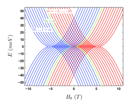
Figure 12: (Color online) The same as Fig. 11, but for $U_{b}=0$ meV.

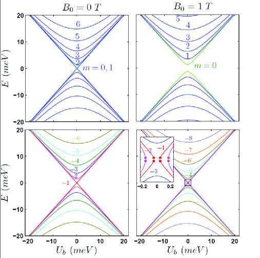
Figure 13: (Color online) Lowest energy levels of a bilayer graphene quantum ring as function of the gate potential $U_{b}$ when $B_{0}=0$ T (left panels) and $B_{0}=1$ T (right panels) for $m\geq 0$ (upper panels) and $m<0$ (Lower panels) with $R=50$ nm.

The dependence of the energy eigenstates on the angular momentum index $m$ is displayed in Fig. 10 for $U_{b}=100$ meV, $R=50$ nm, with $B_{0}=-5$ T (diamonds), $0$ T (circles) and $5$ T (triangles). Due to the finite bias in this case, the fourth-order character of the dispersion Eq. (31) causes the curves to exhibit a Mexican hat shape. The energy minima for $B_{0}=-5,0,5$ T are respectively given by $m=-1,-10,-20$. In Fig. 11 the energy levels are plotted as function of magnetic field, for a quantum ring with $U_{b}=100$ meV, $R=50~{}nm$, and for $-10\leq m\leq-1$ (red curves), $1\leq m\leq 10$ (blue curves), and $m=0$ (green curves). These results are very similar to those found for a finite width ring and exhibit two local minima that are separated by a saddle point. In the case of finite width quantum rings there are additional energy levels correspond with states that are partly localized outside the ring. Figs. 11(a,b) show the asymmetry between the electron and hole states, caused by the bias. It is seen that the electron and hole energies are related by $E_{h}(m,B_{0})=-E_{e}(-m,-B_{0})$, where the indices $h(e)$ refer to holes (electrons). In the absence of bias, the electron-hole symmetry is restored, as shown in Fig. 12, for a ring with $R=50$ nm and the parabolic energy spectrum is recovered with zero energy gap.

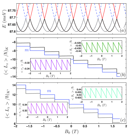
Figure 14: (Color online) (a) Electron energy levels of a bilayer graphene quantum ring as function of external magnetic field $B_{0}$ for a quantum ring of radius $R=50$ nm and with $U_{b}=100~{}meV$ for both the $K$-valley (solid curves) and the $K^{\prime}$-valley (dashed curves). Black curve shows the ground state energy of the energy spectrum in $K$-valley whereas the gray curve the corresponding ground state energy of the $K^{\prime}$-valley (b) Ground state expectation values of $L_{z}/\hbar$, $S_{z}/\hbar$, $\tau_{z}/\hbar$ as function of magnetic field in the $K$-valley. Blue solid curve shows the expectation value of $J_{z}/\hbar$ operator. (c) The same as (b) but, for $K^{\prime}$-valley.

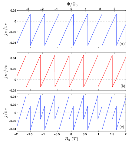
Figure 15: The ground state angular current density in the (a) $K$-valley, (b) $K^{\prime}$-valley and (c) the total current density of a bilayer graphene quantum ring as function of external magnetic field $B_{0}$ with $U_{b}=100$ meV and $R=50$ nm.

In Fig. 13, the energy branches are plotted as function of the bias, for both the zero field case (left panels) and for $B_{0}=1$ T (right panels), with $m\geq 0$ (upper panels) and $m<0$ (lower panels). Notice that the figures are quantitatively similar to those found previously for a quantum ring made of a single layer of graphene where the gate potential $U_{b}$ has a similar effect as the mass term $\Delta$. The differences are that for $B_{0}=0$ T the degeneracies are now: $i$) $E(0)=E(1)=E(-1)$ and $ii$) $E(m)=E(-m)$ for $|m|>1$. In the presence of the magnetic field a gap is opened even for $U_{b}=0$ meV, which is more clearly illustrated in the inset of the right-bottom panel of Fig. 13. Notice that here we found that for $m=-1$ and $m=-2$ no real energy solution is found for $U_{b}$ below some critical value.

Figs. 14(b,c) shows the ground state expectation value of the angular momentum versus the magnetic field together with the quantum number $m$ (blue solid curve) which is an eigenvalue of the total momentum operator $J_{z}$. Notice that the expectation value of $J_{z}$, i.e. $m$, is different in the $K$ and $K^{\prime}$ valley which was not the case for monolayer graphene. The energy levels for the $K$ (solid red curves) and $K^{\prime}$ (dashed blue curves) valleys are depicted in Fig. 14(a). Black curve (gray curve) shows the ground state energy for the $K$-valley ($K^{\prime}$-valley). Notice that in the considered case we find that the difference between $<J_{z}>=m\hbar$ and $<L_{z}>$ is about $(0.7-0.8)\hbar$ for both $K$ and $K^{\prime}$ valleys.

The ground state angular current of a bilayer graphene as function of magnetic field $B_{0}$ in the $K$-valley $j_{K}$, the $K^{\prime}$-valley $j_{K^{\prime}}$ and the total angular current $j$ is shown respectively in Fig 15(a), (b) and (c). In the case of a bilayer graphene quantum ring, the energy levels in the vicinity of the $K$ and $K^{\prime}$ points are different because of the valley splitting and consequently the total angular current versus magnetic field is a more complicated sawtooth function. Notice that the angular current for the $K$ or $K^{\prime}$ valley is not zero at $B_{0}=0$ which is due to the valley polarization whereas the total current is zero at $B_{0}=0$.

IV Summary and conclusions

In summary we considered the behavior of carriers in single and bilayer graphene quantum rings within a toy model. Our approach leads to analytic expressions for the energy spectrum. In our simple model we are not faced with the disadvantages of the nature of edge effects which appears in quantum rings created by cutting the layer of graphene (or lithography defined quantum rings).

We found an interesting new behavior in the presence of a perpendicular magnetic field, which has no analogue in semiconductor-based quantum rings. In single layer graphene quantum rings only for $\Delta>\hbar v_{F}/2R$ we found the opening of a gap in the energy spectrum between the electron and hole states. For both single layer and bilayer graphene quantum rings the eigenvalues are not invariant under a $B_{0}\rightarrow-B_{0}$ transformation and in the case of bilayer the spectra for a fixed total angular momentum index $m$, their field dependence is not parabolic, but exhibit two minima separated by a saddle point. The persistent current exhibits oscillations as function of the magnetic field with period $\Phi_{0}/\pi R^{2}$ which are the well-known Aharonov-Bohm oscillations. Because of the valley splitting in the energy spectrum of bilayer graphene the total current density versus magnetic field is a more complicated sawtooth function.

Acknowledgements This work was supported by the Flemish Science Foundation (FWO-Vl), the Belgian Science Policy (IAP), the Bilateral program between Flanders and Brazil, and the Brazilian Council for Research (CNPq).

References

- (1) Y. Aharonov and D. Bohm, Phys. Rev. 115, 485 (1959).
- (2) Y. Aharonov and A. Casher, Phys. Rev. Lett. 53, 319 (1984).
- (3) A. Fuhrer, S. Lüscher, T. Ihn, T. Heinzel, K. Ensslin, W. Wegscheider, and M. Bichier, Nature (London) 413, 822 (2001).
- (4) K. S. Novoselov, A. K. Geim, S. V. Morozov, D. Jiang, Y. Zhang, S. V. Dubonos, I. V. Grigorieva, and A. A. Firsov, Science, 306, 666 (2004).
- (5) Y. Zhang, Y. W. Tan, H. L. Stormer, and P. Kim, Nature (London) 438, 201 (2005).
- (6) V. P. Gusynin and S. G. Sharapov, Phys. Rev. Lett. 95, 146801 (2005).
- (7) K. S. Novoselov, A. K. Geim, S. V. Morozov, D. Jiang, M. I. Katsnelson, I. V. Grigorieva, S. V. Dubonos, and A. A. Firsov, Nature (London) 438, 197 (2005).
- (8) B. Partoens and F. M. Peeters, Phys. Rev. B 74, 075404 (2006).
- (9) T. Ohta, A. Bostwick, T. Seyller, K. Horn, and E. Rotenberg, Science 313, 951 (2006).
- (10) Edward McCann and Vladimir I. Fal’ko, Phys. Rev. Lett. 96, 086805 (2006).
- (11) S. Russo, J. B. Oostinga, D. Wehenkel, H. B. Heersche, S. S. Sobhani, L. M. K. Vandersypen, and A. F. Morpurgo, Phys. Rev. B 77, 085413 (2008).
- (12) F. Molitor, M. Huefner, A. Jacobsen, A. Pioda, C. Stampfer, K. Ensslin, and T. Ihn, arXiv:0904.1364v1.
- (13) P. Recher, B. Trauzettel, A. Rycerz, Ya. M. Blanter, C. W. Beenakker, and A. F. Morpurgo, Phys. Rev. B 76, 235404 (2007).
- (14) J. Wurm, M. Wimmer, H.U. Baranger, and K.Richter, arXiv:0904.3182v1
- (15) T. Luo, A.P. Iyengar, H.A. Fertig, and L. Brey, arXiv:0907.3150v1
- (16) A. Rycerz, Act. Phys. Pol. A 115, 322 (2009).
- (17) D. A. Bahamon, A. L. C. Pereira, and P. A. Schulz, Phys. Rev. B 79, 125414 (2009).
- (18) M. Zarenia, J. M. Pereira Jr., F. M. Peeters, and G. A. Farias, Nano Lett. 9, 4088, (2009).
- (19) P. Recher, J. Nilsson, G. Burkard, and B. Trauzettel, Phys. Rev. B 79, 085407 (2009).
- (20) F. E. Meijer, A. F. Morpurgo, and T. M. Klapwijk, Phys. Rev. B 66, 033107 (2002).
- (21) B. Molnár, F. M. Peeters, and P. Vasilopoulos, Phys. Rev. B 69, 155335 (2004).
- (22) J. M. Pereira Jr., P. Vasilopoulos, and F. M. Peeters, Nano Lett. 7, 946, (2007).