Positive current cross-correlations in a highly transparent normal-superconducting beam splitter due to synchronized Andreev and inverse Andreev reflections

Abstract

Predictions are established for linear differential current-current cross-correlations $dS_{a,b}/dV$ in a symmetrically biased three-terminal normal metal-superconductor-normal metal (NSN) device. Highly transparent contacts turn out to be especially interesting because they feature positive $dS_{a,b}/dV$. At high transparency, processes based on Crossed Andreev Reflection (CAR) contribute only negligibly to the current and to $dS_{a,b}/dV$. Under these circumstances, current-current cross-correlations can be plausibly interpreted as a coherent coupling between the two NS interfaces in the form of synchronized Andreev and inverse Andreev reflections ($\mathrm{AR}\text{-}\overline{\mathrm{AR}}$), corresponding to the process where a pair of electron-like quasi-particles and a pair of hole-like quasi-particles arrive from the normal electrodes and annihilate in the superconductor. Hence, positive $dS_{a,b}/dV$ does not automatically imply $\mathrm{CAR}$. For tunnel contacts, $dS_{a,b}/dV$ is positive because of $\mathrm{CAR}$. In between these two extremities, at intermediate transparencies, $dS_{a,b}/dV$ is negative because both processes which cause positive correlations, occur only with small amplitude. We use scattering theory to obtain analytic expressions for current and noise, and microscopic calculation using a tight binding model in order to obtain a clear interpretation of the physical processes.

I Introduction

Beautiful experiments on transport and noise in normal metal-superconducting (NS) hybrids allow probing the microscopic physics associated to the superconducting condensate and quasi-particles. For instance, the superconducting gap $\Delta$ was revealed by tunnel spectroscopy on a normal metal-insulator-superconductor tunnel junction. In NS structures with highly transparent contacts, Andreev reflection Andreev is the phenomenon by which pairs of electron-like quasi-particles from the normal electrode N can enter the superconductor S and join the condensate. Additional processes appear in N_aSN_b structures with two normal electrodes N_a and N_b: an electron coming from N_a may be transmitted as an electron into N_b (elastic cotunneling, $\mathrm{EC}$), or it may be transmitted as a hole into N_b (crossed Andreev reflection, $\mathrm{CAR}$Byers ; Deutscher ; Choi ; Falci ; Melin-Feinberg-PRB ; Melin-Duhot-EPJB ; Melin-wl ; Levy-Yeyati ; Golubev ; Kalenkov ; Lambert1 ; Buttiker ; Sols ; Yamashita ; Morten ; Golubov ; Zaikin ; Koltai ; Bednorz ; Giazotto ; Melin-Madrid ; Duhot ; Samuelsson ; ref5 ; ref6-7 ; ref9 ; Bignon ; Melin-Martin ; Faoro ; Russo ; Cadden ; Schonenberger ; Chandra2 ; Beckmann ; Schonenberger2 ). The amplitudes of these two processes decrease exponentially with a characteristic length scale: the coherence length $\xi$, which is inverse proportional to the energy gap $\Delta$ in the ballistic limit. Therefore, three-terminal nanoscale devices with distance $R\gtrsim\xi$ between the contacts are especially interesting: conductance and noise experiments on them probe both the condensate and the quasi-particle states.

Concerning current-current correlations, theorists have envisioned two kinds of experiments for the long term: using entanglement in quantum information devices, and testing entanglement in the electronic Einstein-Podolsky-Rosen (EPR) experiment.Choi ; Martin-Lesovik ; Faoro The EPR experiment is not considered here, but instead the basic problem of current-current cross-correlations Buttiker-revue in NSN structures is addressed. Some experiments based on NISIN structures have been reported recently.Chandra-noise Our task here is not to understand the tunnel limit, where an insulating oxide layer I is inserted in between the normal and the superconducting electrodes, but the opposite limit of highly transparent interfaces where Coulomb interactions Levy-Yeyati are not expected to play a predominant role.

Based on the limiting case of tunnel contacts,Falci ; Bignon one may erroneously conclude that positive differential current-current cross-correlations $dS_{a,b}/dV$ are equivalent to $\mathrm{CAR}$. However, this is not the case because, as we show, positive $dS_{a,b}/dV$ can well be obtained in the absence of $\mathrm{CAR}$.

Current-current cross-correlations are negative Buttiker-prb ; exp1 ; exp2 for non-interacting fermions. A flux of bosons leads to positive cross-correlations HBT and negative cross-correlations are found for bosons impinging one by one onto a beam splitter.Grangier Cross-correlations can be positive in interacting fermionic systems, ref12 ; ref13 ; ref14 ; ref15 ; ref16 ; ref17 ; ref18 as well as in multiterminal NS structures.Duhot ; Samuelsson ; ref5 ; ref6-7 ; ref9 ; Bignon ; Melin-Martin ; Morten ; Bednorz ; Faoro

The recent experiment Chandra-noise and other experiments under way involve normal electrodes separately connected to a superconductor, Melin-Martin with a geometry similar to that considered in the following. Not only the noise can be evaluated in various set-ups, but also the full histogram of the charge transmitted in a given time interval. Bednorz ; Morten ; Faoro In addition to these set-ups, relevant information is also obtained from “zero dimensional” chaotic cavities in contact with a superconductor, in connection with the possibility to observe positive current-current cross-correlations due to $\mathrm{CAR}$. Samuelsson

In what follows, attractive interaction binding pairs of electron-like quasi-particles is present everywhere in the superconducting region. Two electron-like quasi-particles of a pair injected into the superconducting region remain glued by the BCS mean field interaction, in contrast with the dissociation of a Cooper pair entering a chaotic cavity (see Ref. Samuelsson, ). The physics behind current-current cross-correlations in the NSN structure with highly transparent contacts considered here was not really elucidated in Ref. Melin-Martin, , in spite of the important observation that $dS_{a,b}/dV$ is positive but the non-local conductance is negative at low bias. Unusual properties can be realized with the following experimental conditions: First it is assumed that the same voltage $V_{a}=V_{b}\equiv V$ is applied on the two normal electrodes N_a and N_b. Second the temperature is very low, and third high values of interface transparencies are used. Direct electron transmission is Pauli blocked at zero temperature because of the same voltage applied on the two normal electrodes. On the other hand, crossed Andreev reflection is strongly reduced at high transmission, regardless of the applied voltages $V_{a}$ and $V_{b}$. These two features of $\mathrm{EC}$ and $\mathrm{CAR}$ are shown to be a sufficient condition for deducing $dS_{a,b}/dV>0$, not due to $\mathrm{CAR}$, but due to what is called here synchronized Andreev reflection and inverse Andreev reflection ($\mathrm{AR}\text{-}\overline{\mathrm{AR}}$). The positive current-current correlations at high transparency are not in disagreement with what is found in Ref. Samuelsson, for strong coupling to the superconductor, where a gap is induced in a chaotic cavity. The cross-over between high values of interface transparency and tunnel contacts will also be investigated: $\mathrm{CAR}$ has a dominant contribution to $dS_{a,b}/dV$ for tunnel contacts, and $dS_{a,b}/dV$ is negative at the cross-over for intermediate values of interface transparency, where $\mathrm{AR}\text{-}\overline{\mathrm{AR}}$ is suppressed.

The article is divided into two independent main sections where current-current correlations are evaluated on the basis of (i) the scattering approach for a homogeneous superconducting gap (see Sec. III) and of (ii) microscopic calculations taking into account the strong inverse proximity effect (see Sec. IV). Technically, these two sections rely on different approaches and are based on different assumptions. Overall agreement between the two calculations is obtained. Final remarks are provided in Sec. V. Technical details are as much as possible left for Appendices. The article starts with a preliminary section containing definitions and a summary of the main results.

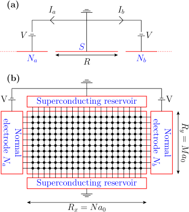
Figure 1: (Color online). The two models studied in this paper: Panel (a) shows the one-dimensional geometry used in the BTK calculation, which is a simplified description for a NSN structure in three dimensions. The central superconducting electrode has length $R$ and the superconducting gap $\Delta_{0}$ is uniform. Panel (b) shows a representation of a three-terminal device described by a tight-binding Hamiltonian. The two superconducting reservoirs have the same phase and thus constitute a single terminal.

II Preliminaries

II.1 Current, noise and current-current correlations

We start with general definitions of current and current-current cross-correlations. The geometry of the considered set-up is shown in Fig. 1. The central island is superconducting, and it is connected by highly transparent contacts to the two superconducting reservoirs on top and bottom. The superconductor S is made of the central island and of the two reservoirs.

The operator giving the current flowing at time $t$ from the normal electrode N_a to the superconducting island S at the N_aS interface [see Fig. 1(b)] takes the form

$$\hat{I}_{a,\alpha}(t) =\sum_{\sigma,n=1}^{M}\left(t_{a_{n},\alpha_{n}}c_{\alpha_{n},\sigma}^{+}(t)c_{a_{n},\sigma}(t)\right.$$ (1)

$$\left.+t_{\alpha_{n},a_{n}}c_{a_{n},\sigma}^{+}(t)c_{\alpha_{n},\sigma}(t)\right),$$

where $\sigma$ is the projection of the spin on the quantization axis and the sum over $n$ runs over the $M$ tight-binding sites describing the interface. Tight-binding sites on the normal side of the interface N_aS are labeled by $a_{n}$, and their counterparts in the superconducting electrode are labeled by $\alpha_{n}$. The hopping amplitudes between electrode N_a and the superconductor are denoted by $t_{a_{n},\alpha_{n}}$ and $t_{\alpha_{n},a_{n}}$. One has $t_{a_{n},\alpha_{n}}=t_{\alpha_{n},a_{n}}\equiv t_{a}$ in the absence of a magnetic field. The average current $I_{a}\equiv\langle\hat{I}_{a,\alpha}(t)\rangle$ is the expectation value of the current operator given by Eq. (1).

Current-current auto-correlations in electrode N_a are given by

$$S_{a,a}(t^{\prime})=\langle\delta\hat{I}_{a}(t+t^{\prime})\delta\hat{I}_{a}(t)\rangle+\langle\delta\hat{I}_{a}(t)\delta\hat{I}_{a}(t+t^{\prime})\rangle,$$ (2)

with $\delta\hat{I}_{a}(t)=\hat{I}_{a}(t)-\langle\hat{I}_{a}(t)\rangle$. In the absence of ac-excitations, the average current given by Eq. (1) is time-independent and the auto-correlations $S_{a,a}(t^{\prime})$ given by Eq. (2) depend only on the difference $t^{\prime}$ of the time arguments.

Similarly, current-current cross-correlations between the electrodes N_a and N_b are given by

$$S_{a,b}(t^{\prime})=\langle\delta\hat{I}_{a}(t+t^{\prime})\delta\hat{I}_{b}(t)\rangle+\langle\delta\hat{I}_{b}(t)\delta\hat{I}_{a}(t+t^{\prime})\rangle,$$ (3)

where $\hat{I}_{b}$ describes the current at the interface with the normal electrode N_b. Zero-frequency auto-correlations ($S_{a,a}$) and cross-correlations ($S_{a,b}$) are defined as the integral over $t^{\prime}$ of $S_{a,a}(t^{\prime})$ and of $S_{a,b}(t^{\prime})$. The definition used here for the Fano factor is as follows: $F_{a,a}=S_{a,a}/2eI_{a}$ and $F_{a,b}=S_{a,b}/2e\sqrt{I_{a}I_{b}}$, with $I_{a}=I_{b}$. With this definition, the Schottky formula leads to $F=q^{*}/e$ for a Poisson process transmitting a charge $q^{*}$.

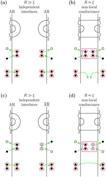
Figure 2: (Color online). Two independent local $\mathrm{AR}$ processes are shown on panel (a), for two interfaces separated by a distance $R$ much larger than the coherence length $\xi$. The labels 1 and 2 on the diagram correspond to electrons and holes respectively. For each $\mathrm{AR}$ process, an electron impinging from the normal electrode onto the interface is converted into a hole, and a pair is transmitted into the superconductor. If $R\sim\xi$, the two $\mathrm{AR}$ processes can be coupled coherently by non-local propagation in the superconductor [see panel (b)], with a quartet as an intermediate state and penetration of a charge $4e$ into the superconductor, which is qualitatively equivalent to double CAR. Panel (c) shows independent $\mathrm{AR}$ and $\overline{\mathrm{AR}}$ processes at the two interfaces, supposed to be far apart. Panel (d) shows $\mathrm{AR}\text{-}\overline{\mathrm{AR}}$ for $R\sim\xi$, which is qualitatively equivalent to double $\mathrm{EC}$.

II.2 Known results and open questions

A few facts related to the non-local conductance for arbitrary values of interface transparency are already known. Only local Andreev reflection $\mathrm{AR}$ and local inverse Andreev reflection $\overline{\mathrm{AR}}$ come into account for contacts separated by a distance much larger than the coherence length [see Figs. 2(a) and (c)]. Local $\mathrm{AR}$ means that an electron is converted into a hole and a pair of electron-like quasi-particles is transmitted into the superconductor, and local $\overline{\mathrm{AR}}$ means that a hole is converted into an electron and a pair of hole-like quasi-particles is transmitted into the superconductor, which annihilates a Cooper pair. Local $\mathrm{AR}$ and $\overline{\mathrm{AR}}$ contribute to transport if the separation between the interfaces is much larger than $\xi$, and in two-terminal configurations where the superconductor is not connected to ground.

Other quantum processes appear in a three-terminal configuration if the distance between the contacts is comparable to the coherence length: $\mathrm{CAR}$ and $\mathrm{EC}$. However, non-standard types of “non-local” processes can be also obtained by merging $\mathrm{AR}$ at the interface N_aS to $\mathrm{AR}$ at the interface SN_b, forming what is called here $\mathrm{AR}\text{-}{\mathrm{AR}}$ [see Fig. 2(b)]. Physically, $\mathrm{AR}\text{-}{\mathrm{AR}}$ would correspond to the synchronized transmission of two pairs from electrodes N_a and N_b into the superconductor, which can be seen as double CAR. However, this process does not contribute to non-local transport at zero temperature. Conversely, $\mathrm{AR}$ at interface N_aS might be associated to $\overline{\mathrm{AR}}$ at interface SN_b, leading to $\mathrm{AR}\text{-}\overline{\mathrm{AR}}$. The corresponding non-local resistance is independent on the value of interface transparency in the tunnel limit. Melin-Duhot-EPJB ; Melin-wl Qualitatively, $\mathrm{AR}\text{-}\overline{\mathrm{AR}}$ can also be seen as double $\mathrm{EC}$.

The non-standard non-local process $\mathrm{AR}\text{-}\overline{\mathrm{AR}}$ involving pairs appears naturally when expanding diagrammatically Melin-wl the non-local conductance to order $t^{8}$, with $t$ the hopping amplitude at the interfaces. As it is shown below, $\mathrm{AR}\text{-}\overline{\mathrm{AR}}$ plays a central role in understanding the positive Melin-Martin current-current cross-correlations for highly transparent contacts, in a regime which is not described by perturbation theory in $t$.

A very recent preprint Che points out the possibility of “synchronized Andreev transmission” in the current-voltage characteristics of a SNS junction array. Synchronization manifests itself in this work as specific features in the current-voltage characteristics of the two-terminal SNS junction array. We arrive here at the conclusion that synchronization of Andreev processes is also possible if the separation between the NS interfaces is comparable to the coherence length. The dominant channel $\mathrm{AR}\text{-}\overline{\mathrm{AR}}$ is shown to result in positive current-current cross-correlations.

As mentioned in the introduction, experiments on current-current cross-correlations in NSN structures have already started.Chandra-noise A few basic questions regarding current-current cross-correlations for highly transparent contacts have not yet received a satisfactory explanation.

First what is the physics behind the positiveMelin-Martin linear differential current-current correlations $dS_{a,b}/dV$ for a highly transparent NSN beam splitter? It is shown that $dS_{a,b}/dV>0$ is not an evidence for $\mathrm{CAR}$ (which would prevail Bignon for tunnel contacts in the absence of Coulomb interactions). An interpretation in terms of $\mathrm{AR}\text{-}\overline{\mathrm{AR}}$ is proposed.

Second, how do current-current cross-correlations depend on the sample geometry? Current-current cross-correlations decay with the geometry-dependent coherence length, as it will be obtained from microscopic calculations in Sec. IV.

Third, what is the value of cross-correlations at intermediate transparencies? Experimentalists can realize tunnel or highly transparent contacts, by oxidizing or not the sample during fabrication. Intermediate values of interface transparency are more difficult to control but it is nevertheless useful to quantify how “perfectly transparent” the NS contacts should be in order to obtain $\mathrm{AR}\text{-}\overline{\mathrm{AR}}$. A cross-over from positive to negative $dS_{a,b}/dV$ is found in BTK calculations as the normal state transmission coefficient $T_{N}$ is reduced below a value typically of order $T_{N}\sim 1/2$.

Fourth, do the predictions established with a ballistic superconductor hold also for a disordered superconductor? It is shown at the end of Sec. IV that, for strong inverse proximity effect, $\mathrm{AR}\text{-}\overline{\mathrm{AR}}$ is responsible for positive cross-correlations also in the case of a disordered superconductor in the regime where the elastic mean free path is shorter than the coherence length.

III Homogeneous superconducting gap: BTK calculation

The BTK approach BTK allows calculations of the current-voltage characteristics of a NS point contact with arbitrary interfacial scattering potential. It was first generalized in Ref. Melin-Duhot-EPJB, and later in Ref. Zaikin, to the case of non-local transport. Useful physical informations can be obtained even though the gap is not self-consistent in the BTK calculation. We will consider a one-dimensional geometry, as shown in Fig. 1(a).

The current $I_{i}$ at the interface with the normal electrode N_i, and the current-current correlations $S_{i,j}$ between the two normal electrodes N_i and N_j are expressedref5 in terms of the scattering matrix $s$ as

$$I_{i} =\frac{e}{h}\int d\omega\sum_{j,\alpha,\beta}\mbox{sgn}(\alpha)\left[\delta_{i,j}\delta_{\alpha,\beta}-\left|s_{i,j}^{\alpha,\beta}\right|^{2}\right]f_{\beta}(\omega)$$ (4)

$$S_{i,j} =\frac{2e^{2}}{h}\int d\omega\sum_{k,l,\alpha,\beta,\gamma,\delta}\mbox{sgn}(\alpha)\mbox{sgn}(\beta)$$ (5)

$$A_{k\gamma,l\delta}(i,\alpha,\omega)A_{l\delta,k\gamma}(j,\beta,\omega)f_{\gamma}(\omega)\left[1-f_{\delta}(\omega)\right],$$

with

$$A_{k\gamma,l\delta}(i,\alpha,\omega)=\delta_{i,k}\delta_{i,l}\delta_{\alpha,\gamma}\delta_{\alpha,\delta}-s_{i,k}^{\alpha,\gamma\dagger}s_{i,l}^{\alpha,\delta}.$$ (6)

Latin labels $i,j,k,l$ run over $a$,$b$, referring to the two normal electrodes N_a and N_b. Greek labels $\alpha,\beta,\gamma,\delta$ denote electrons or holes in the superconductor. The notation $f_{e}(\omega)=\theta(eV-\omega)$ stands for the distribution function of electrons at zero temperature, and $f_{h}(\omega)=\theta(-eV-\omega)$ is the one of holes, where $\theta(x)$ is the Heaviside step-function. In Eqs. (4) and (5), $\mbox{sgn}(\alpha)=+1$ if $\alpha=e$, and $\mbox{sgn}(\alpha)=-1$ if $\alpha=h$.

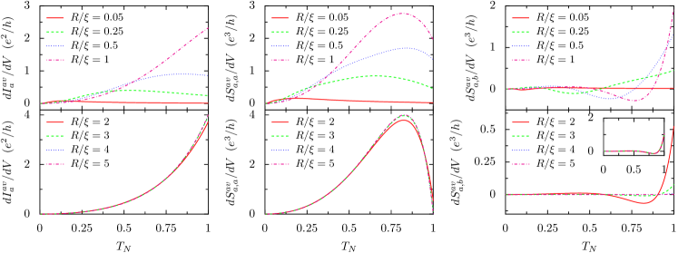
Figure 3: (Color online). Variations of the linear differential conductance [left panels, in units of $e^{2}/h$], linear differential auto-correlations [center panels, in units of $e^{3}/h$] and linear differential cross-correlations [right panels, in units of $e^{3}/h$] as a function of the normal interface transparency $T_{N}$, for the values of $R/\xi$ indicated in the figures. A single-channel one-dimensional BTK calculation is used [see Fig. 1(a)]. The lower Panels show that $dI_{a}^{av}/dV$ and $dS_{a,a}^{av}/dV$ are almost independent on $R/\xi$ for $R/\xi\gtrsim 1$, and that $dS_{a,b}^{av}/dV$ becomes very small as $R/\xi$ increases above $\sim 1$. The insert of the bottom right panel shows the variations of the normalized current-current cross-correlations $[dS_{a,b}^{av}/dV(T_{N})]/[dS_{a,b^{av}}/dV(T_{N}=1)]$. The data corresponding to $R/\xi=2,\,3,\,4,\,5$ superimpose after this rescaling.

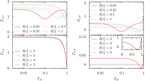
Figure 4: (Color online). Variations of the Fano factors $F_{a,a}=S_{a,a}^{av}/2eI_{a}^{av}$ [top panels] and $F_{a,b}=S_{a,b}^{av}/2eI_{a}^{av}$ [bottom panels] as a function of the normal interface transparency $T_{N}$, for the values of $R/\xi$ indicated in the figures. A single-channel one-dimensional BTK calculation is used [see Fig. 1(a)]. The ratio between the gap $\Delta_{0}$ and the Fermi energy $\epsilon_{F}$ is $\Delta_{0}/\epsilon_{F}=10^{-4}$ in this simulation. The insert of bottom right panel shows the variations of the normalized crossed Fano factor $[F_{a,b}(T_{N})]/[F_{a,b}(T_{N}=1)]$. The data corresponding to $R/\xi=2,\,3,\,4,\,5$ superimpose after rescaling.

The elements of the $s$-matrix are evaluated from the BTK approach (see Appendix A) for a one-dimensional N_aSN_b junction [see Fig. 1(a)]. Step-function variation of the superconducting gap at the interfaces is assumed. A repulsive scattering potential $V(x)=H\left[\delta(x)+\delta(x-R)\right]$ is introduced at the interfaces. The transparency of the interfaces is related to the BTK parameter $Z=H/\hbar v_{F}$, with the Fermi velocity $v_{F}$. The interface transparency is characterized by the value of the normal state transmission coefficient $T_{N}=1/(1+Z^{2})$. Highly transparent contacts correspond to $T_{N}=1$, and tunnel contacts correspond to $T_{N}\ll 1$.

In the one-dimensional model considered in this section, current and noise are highly sensitive to the length $R$ of the superconducting region: they oscillate as a function of $R$ with a period equal to the Fermi wave-length $\lambda_{F}\ll R$. These oscillations can be interpreted as Friedel oscillations where the contacts with the normal electrodes play the role of impurities. In a more realistic higher-dimensional model with more than one transmission mode, the oscillations in the different modes are independent and thus are averaged out. In order to simulate qualitatively multi-dimensional behavior with a one-dimensional system, current and noise are averaged over one oscillation period: Falci ; Melin-Feinberg-PRB ; Melin-Martin

$$I_{i}^{av}(R) =\frac{1}{\lambda_{F}}\int_{R-\lambda_{F}/2}^{R+\lambda_{F}/2}dr\kern 2.0ptI_{i}(r)\,,$$ (7)

$$S_{i,j}^{av}(R) =\frac{1}{\lambda_{F}}\int_{R-\lambda_{F}/2}^{R+\lambda_{F}/2}dr\kern 2.0ptS_{i,j}(r).$$ (8)

In the studied limit of small applied voltage $eV\ll\Delta$, the energy-dependence of the scattering matrix elements can be neglected and $s_{i,j}^{\alpha,\beta}(\omega)\approx s_{i,j}^{\alpha,\beta}(\omega=0)$. Using this approximation, it is possible to perform these integrals analytically.

In this limit, the current $I_{i}$ through the normal lead N_i is obtained as

$$I_{i}^{av}=\frac{2\sqrt{2}e^{2}VT_{N}^{2}(2-T_{N})\cosh(R/\xi)\sinh(R/\xi)^{2}}{h\left[2(2-T_{N})^{2}\cosh(R/\xi)^{2}-8(1-T_{N})\right]^{\frac{3}{2}}}\,.$$ (9)

The local current-current correlations $S_{ii}$ at the interface N_iS and the current-current cross-correlations $S_{ij}$ between the interface N_iS and the interface SN_j are

$$\begin{aligned} S_{ii}^{av}=&\frac{64\sqrt{2}e^{3}VT_{N}^{2}\sinh(R/\xi)^{2}\mathrm{sech}(R/\xi)}{h(2-T_{N})^{3}\left[2(2-T_{N})^{2}\cosh(R/\xi)^{2}-8(1-T_{N})\right]^{\frac{7}{2}}}\\ &\Big{[}-128(1-T_{N})^{4}+2(2-T_{N})^{2}(1-T_{N})(96-T_{N}\\ &\times(192-T_{N}(116-T_{N}(20-3T_{N}))))\cosh(R/\xi)^{2}\\ &-(2-T_{N})^{4}(72-T_{N}(144-T_{N}(82-T_{N}\\ &\times(10+T_{N}))))\cosh(R/\xi)^{4}\\ &+8(2-T_{N})^{6}(1-T_{N})\cosh(R/\xi)^{6}\Big{]}\end{aligned}$$ (10)

and

$$\begin{aligned} S_{i\neq j}^{av}=&\frac{64\sqrt{2}e^{3}VT_{N}^{2}\sinh(R/\xi)^{2}\mathrm{sech}(R/\xi)}{h(2-T_{N})^{3}\left[2(2-T_{N})^{2}\cosh(R/\xi)^{2}-8(1-T_{N})\right]^{\frac{7}{2}}}\\ &\Big{[}128(1-T_{N})^{4}-2(2-T_{N})^{2}(1-T_{N})(2+T_{N})\\ &\times(2-3T_{N})(8-(8-T_{N})T_{N})\cosh(R/\xi)^{2}\\ &+(2-T_{N})^{4}(8-T_{N}(16+T_{N}(2-T_{N}(10+T_{N}))))\\ &\times\cosh(R/\xi)^{4}\Big{]}\,.\end{aligned}$$ (11)

The linear conductance $dI_{a}^{av}/dV$, the auto-correlations $dS_{a,a}^{av}/dV$ and the cross-correlations $dS_{a,b}^{av}/dV$ given by these formulas are shown in Fig. 3 as a function of the normal transmission coefficient $T_{N}$, for different values of the distance between the contacts. As it is expected, the conductance increases with interface transparency for $R/\xi\gtrsim 1$. The conductance depends on the ratio $R/\xi$ while $R$ is smaller than the coherence length $\xi$, but it does almost not vary as $R$ is increased above $\xi$. For $R/\xi<1$, the conductance is non-monotonous when plotted as a function of $T_{N}$ (see Fig. 3 top left). An explanation for the non-monotonous behavior is the enhanced transmission due to the finite size of the superconductor.Beenakker

Starting from tunnel contacts, the linear differential auto-correlation $dS_{a,a}^{av}/dV$ first increases with interface transparency as larger current leads to larger noise. The differential noise reaches a maximum and almost vanishes for perfect transparency if $R\gtrsim\xi$, as it is expected for a single NS junction.Buttiker-revue Differential current-current cross-correlations $dS_{a,b}^{av}/dV$ are positive for $R/\xi\lesssim 1$ in the extreme cases of very high and very low interface transparency, and take negative values in between, as shown in Figs. 3(right), and in the insert of Fig. 3(bottom right).

The Fano factors $F_{a,a}=S_{a,a}^{av}/2eI_{a}^{av}$ and $F_{a,b}=S_{a,b}^{av}/2eI_{a}^{av}$ correspond to the noise normalized to the current, which allows to get rid of the trivial effect that, at low transparency, the noise increases when the current increases. The variations of $F_{a,a}$ and $F_{a,b}$ feature local minima at intermediate values of $T_{N}$. In the insert of Fig. 4(bottom right), the Fano factor $F_{a,b}$ is shown for different $R/\xi\gtrsim 1$. As it can be seen, for $R/\xi\gtrsim 1$ the Fano factor is independent of $R/\xi$ after normalizing to its value for $T_{N}=1$. The Fano factor $F_{a,b}$ is positive outside the region of the minima. For $R/\xi\gtrsim 1$, $F_{a,a}$ takes the value $F_{a,a}\simeq 2$ for $T_{N}\ll 1$, and the value $F_{a,a}\simeq 0$ for $T_{N}=1$.

We first make some remarks in order to confirm the validity of our calculation. Expected behavior is recovered in some known limiting cases:

(i) For tunnel contacts ($T_{N}\ll 1$), the Fano factors are given by $F_{a,a}\approx 2-\frac{1}{2}\mathrm{sech}(R/\xi)$ and $F_{a,b}\approx\frac{1}{2}\mathrm{sech}(R/\xi)$, which is in agreement with the expected limiting values $F_{a,a}=2$ and $F_{a,b}=0$ for $R/\xi\rightarrow\infty$. This corresponds to the doubling of the effective charge for Andreev reflection at a single NS interface in the tunnel limit.Khlus ; Jehl

(ii) For highly transparent interfaces ($T_{N}\approx 1$), the Fano factors vanish exponentially with increasing $R/\xi$ as $F_{a,a}=F_{a,b}\approx\mathrm{sech}(R/\xi)$, as it is expected for a single highly transparent NS interface.

(iii) $dS_{a,b}^{av}/dV$ and $F_{a,b}$ are positive and very small for $R/\xi\gtrsim 1$ and $T_{N}\simeq 1$, in agreement with Ref. Bignon, . Only $\mathrm{CAR}$ contributes to current-current cross-correlations for $T_{N}\ll 1$.

(iv) As it can be seen in Fig. 3(top left), the linear conductance $dI_{a}^{av}/dV$ is suppressed for $R/\xi\lesssim 1$ because the number of normal states within the gap energy is $\sim R/\xi$ for this geometry. For a three-dimensional grain it is proportional to $\sim k_{F}^{2}R^{3}/\xi$, which can be much larger than unity even for $R/\xi\lesssim 1$. The suppression of Andreev processes at high transparency for $R/\xi\ll 1$ is thus not expected to occur in the case of a three-dimensional superconducting grain.

The Schottky limit is realized for low values of interface transparencies, which lead to $\langle(\delta\hat{I}_{a}-\delta\hat{I}_{b})^{2}\rangle_{av}=4eI_{a}^{av}$. On the other hand $\langle(\delta\hat{I}_{a}+\delta\hat{I}_{b})^{2}\rangle_{av}=4e(I_{a}^{av}+I_{b}^{av})$. One concludes that $F_{a,a}\simeq 3/2$ and $F_{a,b}\simeq 1/2$, in agreement with the plateau obtained in Figs. 4(top) for the dependence on $T_{N}$ of the Fano factor. Eqs. (9), (10) and (11) reproduce these values in the limit $R/\xi\rightarrow 0$ and $T_{N}\ll 1$.

For highly transmitting interfaces $T_{N}=1$, we obtain $F_{a,a}=F_{a,b}$. These values can be confirmed by a more simple calculation in the limit $R/\xi\ll 1$ (see Appendix B). The identity $F_{a,a}=F_{a,b}$ implies that $\hat{I}_{a}^{av}-\hat{I}_{b}^{av}$ is noiseless for $T_{N}=1$, independent of $R/\xi$:

$$\int d\tau\langle\left(\delta\hat{I}_{a}(t)-\delta\hat{I}_{b}(t)\right)\left(\delta\hat{I}_{a}(t+\tau)-\delta\hat{I}_{b}(t+\tau)\right)\rangle_{av}$$ (12)

$$=\frac{1}{2}\left(S_{a,a}^{av}+S_{b,b}^{av}-2S_{a,b}^{av}\right)$$

$$=\frac{I_{a}^{av}}{2}\left(F_{a,a}+F_{b,b}-2F_{a,b}\right)=0.$$

By comparison, in a fermionic beam splitter with highly transparent contacts, a charge $e$ transmitted from the source to N_a means no charge transmitted from the source to N_b. Thus, for fermions, it is the sum $\hat{I}_{a}+\hat{I_{b}}$ that is noiseless.

We can see from Fig. 3 that the linear differential cross-correlations of current noise $dS_{a,b}^{av}/dV$ are positive for $T_{N}\ll 1$ and $T_{N}\simeq 1$, while they take negative values in between these two limiting cases. For $T_{N}\ll 1$, the positive $dS_{a,b}^{av}/dV$ can be explained by the presence of CAR processes. This is in agreement with perturbative calculations carried out in Ref. Bignon, . However, for perfectly transmitting interfaces $T_{N}\simeq 1$, CAR processes do not occur, as the elements of the scattering matrix describing CAR (e.g. $s_{a,b}^{e,h}$) equal zero for $T_{N}=1$ (see Appendix B). In this Appendix we obtain in the limit $R/\xi\ll 1$

$$\frac{dS_{a,b}^{av}}{dV} =8\frac{e^{3}}{h}\begin{cases}\left|s_{a,a}^{e,h}\right|^{2}&\text{ for }R/\xi\ll 1\\ \left|s_{a,b}^{e,e}\right|^{2}=T_{\mathrm{EC}}&\text{ for }R/\xi\gtrsim 1\end{cases}$$ (13)

and

$$T_{\mathrm{CAR}} =\left|s_{a,b}^{e,h}\right|^{2}=0.$$ (14)

In section IV, we will use a microscopic model in order to obtain an understanding of the processes contributing to the noise, and to explain $dS_{a,b}^{av}/dV>0$ in the absence of CAR.

To summarize this section, we have obtained analytical expressions for the current and noise in the one-dimensional BTK model. It was shown that $dS_{a,b}^{av}/dV>0$, and that Eq. (13) holds for $R/\xi\gtrsim 1$ and for $T_{N}\simeq 1$. Cooper pair splitting dominates for small normal transmission coefficient $T_{N}\ll 1$, while what will be interpreted in Sec. IV as $\mathrm{AR}\text{-}\overline{\mathrm{AR}}$ dominates for $T_{N}\simeq 1$. These two processes are suppressed for intermediate $T_{N}$, resulting in negative cross-correlations in this parameter range.

IV Microscopic calculations

The current-current cross-correlations for highly transparent interfaces can be further investigated in the two-dimensional tight-binding set-up shown in Fig. 1(b). First, using analytic calculations, we analyze the different contributions to the noise $S_{a,b}$ and show the absence of contributions due to CAR processes. The positive contributions are attributed to processes which we refer to as $\mathrm{AR}\text{-}\overline{\mathrm{AR}}$ (this notation stands for Andreev reflection and inverse Andreev reflection), a denomination which is motivated by the microscopic analysis. Second, numerical calculations are performed, which take into account the inverse proximity effect by determining the gap in a self-consistent manner. In addition, disorder will be included in the calculation. As in the last section, we restrict our study to the case where the same voltages $V_{a}=V_{b}=V$ are applied on both normal leads and $V$ is small compared to the gap $\Delta$.

The expression of current-current cross-correlations $S_{a,b}$ can be decomposed as a sum of six contributions according to the types of transmission modes in the superconductor:

$$S_{a,b}=S_{\mathrm{CAR}}+S_{\mathrm{EC}}+S_{\mathrm{AR}\text{-}\overline{\mathrm{AR}}}+S_{\mathrm{AR}\text{-}{\mathrm{AR}}}+S^{\prime}+S_{\mathrm{MIXED}},$$ (15)

where the expression and the meaning of the different contributions are provided in Appendix D. $S_{\mathrm{CAR}}$ contains the noise attributed to crossed Andreev reflections, which contains transmission modes in the electron-hole channels. $S_{\mathrm{EC}}$, the noise due to elastic cotunneling, contains transmission modes in the electron-electron or hole-hole channels. With ${\mathrm{AR}\text{-}{\mathrm{AR}}}$, we refer to synchronous local Andreev reflections at both interfaces, while ${\mathrm{AR}\text{-}\overline{\mathrm{AR}}}$ links a local Andreev process at one interface to a local inverse Andreev process at the other one (see Fig. 2).

The Andreev-reflection is highly localZaikin (compare with the BTK calculations in Sec. III, where it vanishes exactly). This motivates the assumption $|G_{\alpha,\beta}^{1,2}|\ll|G_{\alpha,\beta}^{1,1}|$, which is confirmed by our numerical calculations also in the presence of the inverse proximity effect (see Fig. 5). Using this simplification, one obtains $S_{\mathrm{CAR}}=S_{\mathrm{AR}\text{-}{\mathrm{AR}}}=0$. The terms $S^{\prime}$ and $S_{\mathrm{MIXED}}$ vanish after integration over the energy $\omega$. Thus the total current-current cross-correlation $S_{a,b}$ depends only on the term $S_{\mathrm{AR}\text{-}\overline{\mathrm{AR}}}$.

Figure 5: (Color online). The anomalous Green function $G_{\alpha_{n},\beta_{m}}^{1,2}$ is small compared to the normal Green function $G_{\alpha_{n},\beta_{m}}^{1,1}$. As the elements $G_{\alpha_{n},\beta_{m}}$ (between site $n$ on the left interface and site $m$ on the right interface) decay exponentially with $d=|y_{n}-y_{m}|$, we have evaluated the mean values $|\langle G_{\alpha_{n},\beta_{m}}|\rangle_{n,m}$ of the elements with the same value of $d$. The main contribution to non-local transport comes from small values of $d$. While the main frame shows the results obtained for a constant gap $\Delta$, the inset shows the corresponding data with the self-consistent gap.

In order to understand what type of microscopic processes are described in $\mathrm{AR}\text{-}\overline{\mathrm{AR}}$, we start from the formula giving the current-current cross-correlations in terms of the Keldysh Green functions $\hat{G}^{+,-}$ and $\hat{G}^{-,+}$:

$$S_{a,b}(\omega)= \mbox{Tr}\left[\hat{G}^{+,-}_{b,a}\hat{G}^{-,+}_{\alpha,\beta}+\hat{G}^{+,-}_{\beta,\alpha}G^{-,+}_{a,b}\right.$$ (16)

$$-\left.\hat{G}^{+,-}_{b,\alpha}\hat{G}^{-,+}_{a,\beta}-\hat{G}^{+,-}_{\beta,a}\hat{G}^{-,+}_{\alpha,b}\right],$$

where the trace is carried out over the Nambu labels and the different transmission modes at the interfaces. It can be shown that all terms in $S_{\mathrm{AR}\text{-}\overline{\mathrm{AR}}}$ are obtained from the anomalous contributions of the type $G^{+,-,1,2}G^{-,+,2,1}$ and $G^{+,-,2,1}G^{-,+,1,2}$. Let us consider one of these terms as an example (the same conclusions are obtained for all terms) and suppose again that $G_{\alpha,\beta}^{A,1,2}=0$ if $\alpha$ and $\beta$ are on different interfaces (that is, crossed Andreev reflection does not contribute), and that a symmetric bias voltage is applied on the two normal electrodes. One has

$$G^{+,-,2,1}_{b,a}(t,t^{\prime})G^{-,+,1,2}_{\alpha,\beta}(t^{\prime},t)$$ (17)

$$=\langle c_{a,\downarrow}(t^{\prime})c_{b,\uparrow}(t)\rangle\langle c_{\beta,\uparrow}^{+}(t^{\prime})c_{\alpha,\downarrow}^{+}(t)\rangle.$$

This equation can be understood as a relation between initial and final states, as it is shown in Fig. 6. In general, these states can be connected by many different processes. However, the microscopic formula for the current-current cross-correlations [see Eq. (46)] shows that the initial and final states are related by an Andreev process at interface N_aS, and, at the same time, by an inverse Andreev process at interface SN_b [see Fig. 6(b)]. In an Andreev process, an electron is converted into a hole and a pair of electron-like quasi-particles is transmitted into the superconductor. In an inverse Andreev process, a hole is converted into an electron and a pair of hole-like quasi-particles is transmitted into the superconductor. The pair of electron-like quasi-particles annihilates with the pair of hole-like quasi-particles and the remaining electron and the hole are exchanged between the two interfaces. This results in $dS_{\mathrm{AR}\text{-}\overline{\mathrm{AR}}}/dV>0$.

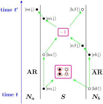
Figure 6: (Color online). Schematic representation of how $\mathrm{AR}\text{-}\overline{\mathrm{AR}}$ couples to current-current cross-correlations. The initial state consists of (i) a spin-down electron created at $\alpha$ at time $t$, on the superconducting side of the N_aS interface, and of (ii) a spin-up electron destroyed at time $t$ at b, on the normal side of interface SN_b. The final state consists of a spin-down electron destroyed at time $t^{\prime}$ at a, on the normal side of interface N_aS, and of a spin-up electron created at time $t^{\prime}$ at $\beta$, on the superconducting side of interface SN_b. To the $\mathrm{AR}\text{-}\overline{\mathrm{AR}}$ process shown on Fig. 2d, the permutation of two fermions is added. Taking into account the resulting minus sign leads to positive current-current cross-correlations.

Figure 7: (Color online). The figure shows $dS_{a,b}/dV$ as a function of $N$ for highly transmitting interfaces [for $N$ see Fig. 1(b)]. In agreement with the BTK calculations $dS_{a,b}/dV>0$. The exponential decay is described by the coherence length which increases with $M$, in agreement with Ref. Melin-Madrid, . The values $M=20$ (red squares) and $M=25$ (blue circle) are used. Strong deviations from the exponential decay (red lines) appear for $N\simeq M$ (see Ref. Melin-Madrid, ). The data points are obtained from Eq. (42). The decay is $\propto\exp[-2Na_{0}/\xi(M)]$.

In addition to the analytic calculation, we performed numerical simulations in order to analyze a more realistic model. Details about the used method Melin-Madrid are presented in Appendix C. The self-consistent simulations presented below take into account the inverse proximity effect corresponding to the reduction of the superconducting gap within a distance $\sim\xi$ from the contacts. Self-consistency is equivalent to current conservation for the electrons injected from the normal reservoirs and transmitted into the superconducting ones.

The values for the linear differential cross-correlations $dS_{a,b}/dV$, and for the $\mathrm{EC}$ and $\mathrm{CAR}$ transmission coefficients $T_{\mathrm{EC}}$ and $T_{\mathrm{CAR}}$ are plotted as functions of the length $N$ of the superconductor in Figs. 7 and 8. The notations $T_{\mathrm{EC}}$ and $T_{\mathrm{CAR}}$ refer to the transmission modes in the superconductor (advanced-advanced or retarded-retarded modes not exchanging electrons and holes for $T_{\mathrm{EC}}$, and advanced-retarded Green functions exchanging electrons and holes for $T_{\mathrm{CAR}}$). $T_{\mathrm{EC}}$ and $T_{\mathrm{CAR}}$ are given by

$$T_{\mathrm{EC}} =W^{2}\text{Tr}\left(G^{A,1,1}_{\alpha,\beta}G^{R,1,1}_{\beta,\alpha}+G^{A,2,2}_{\alpha,\beta}G^{R,2,2}_{\beta,\alpha}\right)$$ (18)

$$T_{\mathrm{CAR}} =W^{2}\text{Tr}\left(G^{A,1,2}_{\alpha,\beta}G^{R,2,1}_{\beta,\alpha}+G^{A,2,1}_{\alpha,\beta}G^{R,1,2}_{\beta,\alpha}\right),$$ (19)

where $W$ is the hopping amplitude in the bulk and at the interfaces, and $\alpha_{n}$ and $\beta_{m}$ run respectively over all the sites on the superconducting side of the N_aS and SN_b interfaces. The notation $G_{i,j}^{A(R),n_{i},n_{j}}$ stands for the Nambu component $(n_{i},n_{j})$ of the advanced (retarded) Green function connecting $i$ to $j$.

Figure 8: (Color online). The exponential decay of the $\mathrm{EC}$ transmission coefficient $T_{\mathrm{EC}}$ [Eq. (18), open red squares for $M=20$ and open blue circles for $M=25$], and of the crossed Andreev transmission coefficient $T_{\mathrm{CAR}}$ [Eq. (19), filled green squares for $M=20$ and filled purple circles for $M=25$] is shown. The decay is $\propto\exp[-2Na_{0}/\xi(M)]$, with $\xi(20)=8a_{0}$ and $\xi(25)=9a_{0}$.

The dependence on $M$ of the coherence length was already found in a previous work.Melin-Madrid The differential cross-correlations $dS_{a,b}/dV$ are positive, which is in agreement with the preceding BTK calculation. Differential cross-correlations $dS_{a,b}/dV$ show exponential decay (see Fig. 7) as a function of $N$, because the two normal electrodes N_a and N_b are coherently coupled by evanescent states in the superconductor. The BCS coherence length as obtained from the fits fulfills $R_{x}/\xi\gtrsim 1$ in a wide range of simulation parameters. This is the range in which the BTK calculation leads to $dS_{a,b}^{av}/dV=8\frac{e^{3}}{h}T_{\mathrm{EC}}$.

For a highly transparent NS contact, one has $G_{\alpha_{n},\alpha_{n}}^{2,1}G_{\beta_{m},\beta_{m}}^{1,2}\simeq 1/4W^{2}$ where $W$ is the hopping amplitude in the normal and superconducting electrodes, and at the interface (see Appendix E). The identity $T^{A,A}_{\mathrm{AR}\text{-}\overline{\mathrm{AR}}}\simeq T_{EC}$ holds if $|G_{\alpha,\beta}^{1,2}|\ll|G_{\alpha,\beta}^{1,1}|$ (see Appendix E), with

$$T_{\mathrm{AR}\text{-}\overline{\mathrm{AR}}}^{A,A}=-W^{2}\text{Tr}\left(G^{A,1,1}_{\alpha,\beta}G^{A,2,2}_{\beta,\alpha}+G^{A,2,2}_{\alpha,\beta}G^{A,1,1}_{\beta,\alpha}\right),$$ (20)

where the superscript “A,A” refers to an advanced-advanced transmission mode where electrons and hole are conserved. With these assumptions, the total noise can be written as

$$\frac{dS_{a,b}}{dV} \simeq 8\frac{e^{3}}{h}T^{A,A}_{\mathrm{AR}\text{-}\overline{\mathrm{AR}}}\,,$$ (21)

$$T^{A,A}_{\mathrm{AR}\text{-}\overline{\mathrm{AR}}} \simeq T_{\mathrm{EC}}.$$ (22)

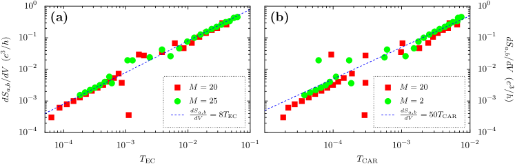
Figure 9: (Color online). Relation between $dS_{a,b}/dV$ and the transmission coefficients $T_{\mathrm{EC}}$ and $T_{\mathrm{CAR}}$: Panel (a) shows the relation between $dS_{a,b}/dV$ and $T_{\mathrm{EC}}$ and panel (b) shows the relation between $dS_{a,b}/dV$ and $T_{\mathrm{CAR}}$. The data are the same as in Fig. 7. The different points correspond to different lengths $N$ along $Ox$ axis [see $N$ in Fig. 1(b)]. The blue dashed lines show the linear fits $dS_{a,b}/dV=8T_{\mathrm{EC}}$, and $dS_{a,b}/dV=50T_{\mathrm{CAR}}$.

Considering the numerical data, plots of $dS_{a,b}/dV$ as functions of $T_{\mathrm{EC}}$ and $T_{\mathrm{CAR}}$ (see Fig. 9), and a comparison between $T_{\mathrm{AR}\text{-}\overline{\mathrm{AR}}}^{A,A}$ and $T_{\mathrm{EC}}$ confirm Eqs. (21) and (22) and show in addition

$$\frac{dS_{a,b}}{dV}\simeq 50\frac{e^{3}}{h}T_{\mathrm{CAR}}.$$ (23)

Comparing with the previous BTK calculation, it is suggested that Eq. (23) is model-dependent, because $T_{\mathrm{CAR}}=0$ for the BTK model while $T_{\mathrm{CAR}}$ is finite but small in the self-consistent microscopic calculation. On the other hand, Eq. (21), which is obtained also for the BTK model, is expected to be a fundamental relation.

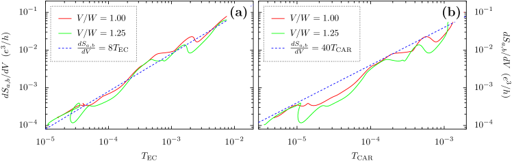
Figure 10: (Color online). Relation between $dS_{a,b}/dV$ and the transmission coefficients $T_{\mathrm{EC}}$ and $T_{\mathrm{CAR}}$ in the presence of weak disorder ($V/W=1$ and $V/W=1.25$): Panel (a) shows the relation between $dS_{a,b}/dV$ and $T_{\mathrm{EC}}$ and panel (b) shows the relation between $dS_{a,b}/dV$ and $T_{\mathrm{CAR}}$. The figure is obtained by averaging over the contributions between the combinations of all different transverse sites $x_{n}$ and $x_{m}$ in the two normal leads. The width of the model is given by $M=20$ [see $M$ in Fig. 1(b)].

Until now, we only studied perfect systems without disorder. The numerical calculations based on microscopic Green functions give us however the additional possibility to add disorder to the model, which is an unavoidable ingredient to describe experiments.

Eq. (21) remains approximately valid in the presence of weak disorder (see Fig. 10), introduced in the form of a random on-site potential uniformly distributed in the interval $\left[-V,V\right]$, with elastic mean free path $l_{e}\sim(W/V)^{2}a_{0}$ smaller than the ballistic coherence length $\sim(W/\Delta)a_{0}$, but not small compared to the Fermi wave-length. The parameter $W$ is the hopping amplitude in the bulk of the superconductor, taking the same value at the interfaces because of highly transparent contacts.

The coherence length is reduced as the strength of disorder increases. The coherence lengths are fitted to $\xi=3.8a_{0},\,3.6a_{0}$ for $V/W=1.00,\,1.25$, as compared to $\xi=8a_{0}$ with $V/W=0$ in the ballistic limit. The coherence length in the presence of disorder becomes smaller than its ballistic value, as for a superconductor in the dirty limit. Within error-bars, Eq. (21) is fulfilled also in the presence of weak disorder, while the coefficient in Eq. (22) is changed, resulting in

$$\frac{dS_{a,b}}{dV}\simeq 40\frac{e^{3}}{h}T_{\mathrm{CAR}}.$$ (24)

It is concluded that $T_{\mathrm{CAR}}\ll T_{\mathrm{EC}}$ implies that $S_{a,b}\simeq S_{a,b}^{\mathrm{AR}\text{-}\overline{\mathrm{AR}}}$ and that Eq. (21) is fulfilled. Thus, it was shown that, in this parameter regime, $dS_{a,b}/dV>0$ is evidence for $\mathrm{AR}\text{-}\overline{\mathrm{AR}}$, not for $\mathrm{CAR}$.

The BTK approach and the microscopic calculations lead to positive $dS_{a,b}/dV>0$, which is due to the exchange of fermionic quasi-particles (see Fig. 6). This is the main physical result of our article: $dS_{a,b}/dV>0$ at high transparency is not due to CAR. It is due to pairs of electron-like quasi-particles, pairs of hole-like quasi-particles, and exchange of fermions.

V Conclusions

The article was already summarized in Sec. II.2 and thus we conclude with a brief overview and final remarks. We have evaluated current-current cross-correlations in a NSN structure with a homogeneous superconductor (without self-consistency in the order parameter), and with strong inverse proximity effect (with self-consistent microscopic calculations for a two-dimensional three-terminal set-up). For both approaches, the linear differential cross-correlations $dS_{a,b}/dV$ are positive for highly transparent contacts and decay exponentially with a characteristic length set by the coherence length. Positive $dS_{a,b}/dV$ arises in this set-up not because of $\mathrm{CAR}$, but because of what is identified as the correlated penetration of pairs of electron-like quasi-particles and pairs of hole-like quasi-particles into the superconductor in the form of $\mathrm{AR}\text{-}\overline{\mathrm{AR}}$. The positive sign of $dS_{a,b}/dV$ is due to the additional exchange of two fermions. It is emphasized that the proposed mechanism does not involve quartets in the superconductor, because $\mathrm{AR}\text{-}{\mathrm{AR}}$ does not contribute to the current-current cross-correlations. Direct evaluation of $dS_{a,b}/dV$ leads to $dS_{a,b}/dV=4(e^{3}/h)T^{A,A}_{\mathrm{AR}\text{-}\overline{\mathrm{AR}}}$, and to $T^{A,A}_{\mathrm{AR}\text{-}\overline{\mathrm{AR}}}\simeq T_{EC}$, which holds also for a superconductor with weak disorder and with elastic mean free path shorter than the coherence length.

Finally, correlations between pairs of Andreev pairs were discussed Nazarov ; Heikkila in connection with noise in an Andreev interferometer.

Future studies of this class of set-ups might include the effect of arbitrary applied voltages and quantitative effects of three-dimensional geometry.

Appendix A Details on the scattering approach

The elements $s_{i,j}^{\alpha,\beta}$ of the scattering matrix are calculated within the BTK approachBTK using two-component wave-functions describing electrons and holes respectively. The indices $i,j$ refer to the normal electrodes N_a and N_b, while $\alpha,\beta$ run over the two components describing the electrons and holes.

For example, the wave-functions for an electron incoming from electrode N_a take the form

$$\psi_{a}(x) =\begin{aligned} &\begin{pmatrix}1\\ 0\end{pmatrix}\left(e^{iq^{(+)}x}+s^{e,e}_{a,a}e^{-iq^{(+)}x}\right)\\ &+s^{h,e}_{a,a}\begin{pmatrix}0\\ 1\end{pmatrix}e^{iq^{(-)}x}\,,\end{aligned}$$ (25)

$$\psi_{S}(x) =\begin{aligned} &\begin{pmatrix}u_{0}\\ v_{0}\end{pmatrix}\left(c_{1}e^{ik^{(+)}x}+c^{\prime}_{1}e^{-ik^{(+)}(x-R)}\right)\\ &+\begin{pmatrix}v_{0}\\ u_{0}\end{pmatrix}\left(d_{1}e^{-ik^{(-)}x}+d^{\prime}_{1}e^{ik^{(-)}(x-R)}\right)\,,\end{aligned}$$ (26)

$$\psi_{b}(x) =\begin{aligned} &\begin{pmatrix}0\\ 1\end{pmatrix}s^{h,e}_{b,a}e^{-iq^{(-)}(x-R)}+\begin{pmatrix}1\\ 0\end{pmatrix}s^{e,e}_{b,a}e^{iq^{(+)}(x-R)},\end{aligned}$$ (27)

where $\psi_{a}(x)$, $\psi_{S}(x)$ and $\psi_{b}(x)$ are the parts of the wave-functions in the electrodes N_a, S, and N_b respectively [see Fig. 1(a)]. The notations $q^{(+)}$, $q^{(-)}$, $k^{(+)}$ and $k^{(-)}$ stand for the wave-vectors in the normal and superconducting electrodes:

$$k^{(\pm)} =k_{F}\pm i/\xi$$ (28)

$$q^{(\pm)} =k_{F}\,,$$ (29)

with $k_{F}\xi\gg 1$.

The elements $s^{e,e}_{a,a}$, $s^{h,e}_{a,a}$, $s^{h,e}_{b,a}$ and $s^{e,e}_{b,a}$ can be determined using the continuity of the wave-functions at the interfaces [$\psi_{a}(0)=\psi_{S}(0)$ and $\psi_{S}(R)=\psi_{b}(R)$] and the boundary condition for the derivatives [$\psi_{S}^{\prime}(0)-\psi_{a}^{\prime}(0)=H\psi_{a}(0)$ and $\psi_{b}^{\prime}(R)-\psi_{S}^{\prime}(R)=H\psi_{b}(R)$]. The BTK parameter $Z$ is defined by $Z=H/\hbar v_{F}$.

The remaining elements of the scattering matrix can be obtained from the other possible scattering processes (e.g., a hole incoming from electrode N_b) by analogous calculation.

By comparing the different equations, the symmetry

$$s_{a,a}^{e,h}(\omega)=\overline{s_{b,b}^{h,e}(-\omega)}$$ (30)

of the scattering matrix can be obtained.

The BCS coherence factors $u_{0}$, $v_{0}$ appearing in these equations are given by:

$$u_{0}^{2}=1-v_{0}^{2}=\frac{1}{2}\left(1+\frac{\sqrt{\omega^{2}-\Delta^{2}}}{\omega}\right).$$ (31)

The coherence factors $u_{0}$ and $v_{0}$ are interchanged under complex conjugation and changing sign of the real part of energy (a small imaginary part is supposed to be added to $\omega$).

Appendix B Current-current cross-correlations for the BTK model in the limit $Z\simeq 0$

For highly transparent interfaces ($Z\simeq 0$), the expressions obtained for $s_{i,j}^{\alpha,\beta}$ simplify considerably, local reflections ($s_{i,i}^{\alpha,\alpha}=0$) and non-local Andreev reflections ($s_{i,j}^{\alpha,\beta}=0$, with $i\neq j,\alpha\neq\beta$) are suppressed. Zaikin Thus, only local Andreev reflection ($s_{i,i}^{\alpha,\beta}$, with $\alpha\neq\beta$) and transmission without branch-crossing ($s_{i,j}^{\alpha,\alpha}$, with $i\neq j$) can occur. The non-zero elements of the scattering matrix are given by

$$s_{a,a}^{h,e} =u_{0}v_{0}\frac{e^{R/\xi}-e^{-R/\xi}}{v_{0}^{2}e^{R/\xi}-u_{0}^{2}e^{-R/\xi}}\,,$$ (32)

$$s_{b,a}^{e,e} =e^{-ik_{F}R}\frac{u_{0}^{2}-v_{0}^{2}}{u_{0}^{2}e^{-R/\xi}-v_{0}^{2}e^{R/\xi}}\,.$$ (33)

Assuming $s(\omega)$ to be constant in the range $[-eV,eV]$ (we study the case $eV\ll\Delta$), Eqs. (4) and (5) can be written as

$$I_{a} =\frac{4e^{2}}{h}V\left|s^{e,h}_{a,a}\right|^{2}\,,$$ (34)

$$S_{a,b} =-\frac{4e^{3}}{h}|V|\left(s_{a,b}^{h,h\dagger}s_{b,b}^{h,e}s_{b,a}^{e,e}s_{a,a}^{e,h\dagger}+s_{a,a}^{h,e\dagger}s_{a,b}^{e,e}s^{e,h}_{b,b}s^{h,h\dagger}_{b,a}\right)$$ (35)

for $i\neq j$. In the limit $R/\xi\ll 1$, the elements of the scattering matrix (evaluated for $\omega\rightarrow 0$) are given by

$$s_{a,a}^{h,e} =s_{b,b}^{e,h}\simeq i\frac{R}{\xi}\,,$$ (36)

$$s_{b,a}^{e,e}s_{a,b}^{h,h} \simeq 1,$$ (37)

leading to

$$S_{a,a}=S_{a,b}=\frac{8e^{3}}{h}|V|\left(\frac{R}{\xi}\right)^{2}\geq 0\,.$$ (38)

The result for $S_{a,a}$ is obtained by an analogous calculation.

Combining Eq. (34) for $I_{a}$ with Eq. (38) for $S_{a,a}$ and $S_{b,b}$ leads to $F_{a,a}\simeq F_{b,b}\simeq 1$ for $eV\ll\Delta_{0}$, $T_{N}=1$ and $R/\xi\ll 1$.

Appendix C Technical details on microscopic calculations

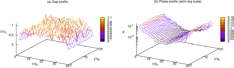
Figure 11: (Color online). The figure shows the gap profile in panel (a), the phase profile in semi-log scale in panel (b), for a given realization of disorder with $V/W=1$. See the text for the meaning of the parameters $V$ and $W$. The $x$ and $y$ axis are the same as in Fig. 1(b). This figure is obtained with the self-consistent algorithm developed in Ref. Melin-Madrid, for the ballistic case. The phase in panel (b) is small but non-zero because the algorithm takes into account non-equilibrium effects.

The microscopic calculations are based on the following tight-binding Hamiltonian on a square lattice:

$${\cal H}_{S}= -W\sum_{\langle n,m\rangle}\sum_{\sigma}\left(c_{n,\sigma}^{+}c_{m,\sigma}+c_{m,\sigma}^{+}c_{n,\sigma}\right)$$ (39)

$$+\sum_{n}\Delta_{n}\left(c_{n,\uparrow}^{+}c_{n,\downarrow}^{+}+c_{n,\downarrow}c_{n,\uparrow}\right)$$

$$-\sum_{n,\sigma}V_{n}c_{n,\sigma}^{+}c_{n,\sigma},$$

with the hopping amplitude $W$ between nearest neighbor sites $n$ and $m$ separated by a distance $a_{0}$. The normal electrodes are described by an analogous Hamiltonian with no pairing term and no disorder. Highly transparent contacts with interfacial hopping equal to $W$ are used in Sec. IV. The parameter $\Delta_{n}$ is the superconducting order parameter at site $n$. It is determined self-consistently in Sec. IV on the basis of the recursive algorithm developed in Ref. Melin-Madrid, . The gap in the superconducting reservoirs takes the fixed value $\Delta_{0}$. Disorder is introduced at the end of Sec. IV in the form of a random on-site potential $V_{n}$ on each tight-binding site, uniformly distributed in the interval $\left[-V,V\right]$. The gap and phase profiles in the superconducting island are shown in Fig. 11 in order to illustrate the output of the part of the code performing the self-consistent calculation. Because of disorder, the gap fluctuates strongly from one tight-binding site to the next. The phase profile shows a smooth exponential decay from the NS interfaces. The accuracy of the self-consistent calculation gives access to variations of the phase over almost two orders of magnitude.

The average current in Eq. (1) is evaluated from the Keldysh Green function:Cuevas

$$I_{a,\alpha}=\frac{2e}{h}\sum_{m}\int d\omega\Big{[} \hat{t}_{a_{m},\alpha_{m}}\hat{G}^{+,-}_{\alpha_{m},a_{m}}(\omega)$$ (40)

$$-\hat{t}_{\alpha_{m},a_{m}}\hat{G}^{+,-}_{a_{m},\alpha_{m}}(\omega)\Big{]}_{1,1}.$$

Zero frequency noise (see Sec. II) is obtained from $S_{a,a}=2e^{2}t^{2}/h\int d\omega S_{a,a}(\omega)$ and $S_{a,b}=2e^{2}t^{2}/h\int d\omega S_{a,b}(\omega)$, with

$$S_{a,a}(\omega)= \sum_{n,m}\mbox{Tr}\Big{[}\begin{aligned} &\hat{G}^{+,-}_{a_{m},a_{n}}(\omega)\hat{G}^{-,+}_{\alpha_{n},\alpha_{m}}(\omega)\\ &+\hat{G}^{+,-}_{\alpha_{m},\alpha_{n}}(\omega)\hat{G}^{-,+}_{a_{n},a_{m}}(\omega)\\ &-\hat{G}^{+,-}_{a_{m},\alpha_{n}}(\omega)\hat{G}^{-,+}_{a_{n},\alpha_{m}}(\omega)\\ &-\hat{G}^{+,-}_{\alpha_{m},a_{n}}(\omega)\hat{G}^{-,+}_{\alpha_{n},a_{m}}(\omega)\Big{]}\,,\end{aligned}$$ (41)

$$S_{a,b}(\omega)= \sum_{n,m}\mbox{Tr}\Big{[}\begin{aligned} &\hat{G}^{+,-}_{b_{m},a_{n}}(\omega)\hat{G}^{-,+}_{\alpha_{n},\beta_{m}}(\omega)\\ &+\hat{G}^{+,-}_{\beta_{m},\alpha_{n}}(\omega)\hat{G}^{-,+}_{a_{n},b_{m}}(\omega)\\ &-\hat{G}^{+,-}_{b_{m},\alpha_{n}}(\omega)\hat{G}^{-,+}_{a_{n},\beta_{m}}(\omega)\\ &-\hat{G}^{+,-}_{\beta_{m},a_{n}}(\omega)\hat{G}^{-,+}_{\alpha_{n},b_{m}}(\omega)\Big{]}.\end{aligned}$$ (42)

The trace is evaluated over the Nambu labels. Eq. (42) is a generalization of Ref. Cuevas-noise, to two interfaces with many channels. The numerical calculations presented in the main body of the article are based on Eqs. (40), (41) and (42).

Appendix D Microscopic calculations for the noise formula

In this Appendix we provide the complete formula for the noise $S_{a,b}(\omega)$ given by Eq. (42) for sub-gap voltage ($|\omega|<eV<\Delta$). This allows considerable simplification of the expression of $S_{a,b}$ because the Keldysh Green function $g^{+-}=0$ in the isolated superconductor, as there exist no single-electron states. The total noise can be decomposed into different terms according to the types of transmission modes in the superconductor as:

$$S_{a,b}(\omega)=S_{\mathrm{CAR}}+S_{\mathrm{EC}}+S_{\mathrm{AR}\text{-}\overline{\mathrm{AR}}}+S_{\mathrm{AR}\text{-}{\mathrm{AR}}}+S_{\mathrm{MIXED}}+S^{\prime}.$$ (43)

In the normal lead $N$, the Keldysh Green functions read $g^{+-,11}_{NN}=2i\pi\rho_{N}n_{F}(\omega-eV)$, $g^{+-,22}_{NN}=2i\pi\rho_{N}n_{F}(\omega+eV)$, $g^{-+,11}_{NN}=2i\pi\rho_{N}n_{F}(-\omega+eV)$ and $g^{-+,22}_{NN}=2i\pi\rho_{N}n_{F}(-\omega-eV)$, where $\rho_{N}$ is the density of states at the interface in the normal lead, and, at zero temperature, $n_{F}(x)=\theta(-x)$, with $\theta(x)$ being the Heaviside step-function. This gives $g^{+-,11}_{N,N}g^{-+,22}_{N,N}=g^{+-,22}_{N,N}g^{-+,11}_{N,N}=0$, leading to further simplification of the expression for $S_{a,b}$.

The contribution $S_{\mathrm{CAR}}$ is given by the advanced-advanced or retarded-retarded transmission modes in the electron-hole channel, in the form of the combinations of the type $G^{A,12}_{\alpha\beta}G^{R,21}_{\beta\alpha}$. Physically, these microscopic processes can be interpreted as Cooper pair splitting as appearing in $\mathrm{CAR}$. The expression for $S_{\mathrm{CAR}}$ is as follows:

$$S_{\mathrm{CAR}}=2t^{4}\Big{[} +g^{-+,11}_{bb}g^{+-,22}_{aa}G^{R,21}_{\alpha\beta}G^{R,12}_{\beta\alpha}(1+2iG^{A,22}_{\alpha\alpha}\pi t^{2}\rho_{a})(1+2iG^{A,11}_{\beta\beta}\pi t^{2}\rho_{b})$$ (44)

$$+g^{-+,22}_{bb}g^{+-,11}_{aa}G^{R,12}_{\alpha\beta}G^{R,21}_{\beta\alpha}(1+2iG^{A,11}_{\alpha\alpha}\pi t^{2}\rho_{a})(1+2iG^{A,22}_{\beta\beta}\pi t^{2}\rho_{b})$$

$$-g^{-+,22}_{aa}g^{+-,11}_{bb}G^{A,21}_{\alpha\beta}G^{A,12}_{\beta\alpha}(i+2G^{R,22}_{\alpha\alpha}\pi t^{2}\rho_{a})(i+2G^{R,11}_{\beta\beta}\pi t^{2}\rho_{b})$$

$$-g^{-+,11}_{aa}g^{+-,22}_{bb}G^{A,12}_{\alpha\beta}G^{A,21}_{\beta\alpha}(i+2G^{R,11}_{\alpha\alpha}\pi t^{2}\rho_{a})(i+2G^{R,22}_{\beta\beta}\pi t^{2}\rho_{b})\Big{]}\,,$$

where $t$ is the hopping amplitude at the interfaces.

The contribution $S_{\mathrm{EC}}$ contains advanced-advanced and retarded-retarded transmission modes in the electron-electron or hole-hole channel, in the form of the combinations of the type $G^{A,12}_{\alpha\beta}G^{A,21}_{\beta\alpha}$. This is the contribution to the noise of normal electron transmission in the form of $\mathrm{EC}$. The expression reads

$$S_{\mathrm{EC}}=2t^{4}\Big{[} +g^{-+,11}_{bb}g^{+-,11}_{aa}G^{R,11}_{\alpha\beta}G^{R,11}_{\beta\alpha}(i-2G^{A,11}_{\alpha\alpha}\pi t^{2}\rho_{a})(i-2G^{A,11}_{\beta\beta}\pi t^{2}\rho_{b})$$ (45)

$$+g^{-+,22}_{bb}g^{+-,22}_{aa}G^{R,22}_{\alpha\beta}G^{R,22}_{\beta\alpha}(i-2G^{A,22}_{\alpha\alpha}\pi t^{2}\rho_{a})(i-2G^{A,22}_{\beta\beta}\pi t^{2}\rho_{b})$$

$$+g^{-+,11}_{aa}g^{+-,11}_{bb}G^{A,11}_{\alpha\beta}G^{A,11}_{\beta\alpha}(i+2G^{R,11}_{\alpha\alpha}\pi t^{2}\rho_{a})(i+2G^{R,11}_{\beta\beta}\pi t^{2}\rho_{b})$$

$$+g^{-+,22}_{aa}g^{+-,22}_{bb}G^{A,22}_{\alpha\beta}G^{A,22}_{\beta\alpha}(i+2G^{R,22}_{\alpha\alpha}\pi t^{2}\rho_{a})(i+2G^{R,22}_{\beta\beta}\pi t^{2}\rho_{b})\Big{]}\,.$$

Now we consider processes that do not appear in lowest order perturbation theory. First the contribution $S_{\mathrm{AR}\text{-}\overline{\mathrm{AR}}}$ contains advanced-advanced and retarded-retarded transmission modes, in the form of the combinations of the type $G^{A,11}_{\alpha\beta}G^{A,22}_{\beta\alpha}$. Physically, this can be interpreted as the contribution to the noise of synchronized Andreev and inverse Andreev processes ($\mathrm{AR}\text{-}\overline{\mathrm{AR}}$), with the exchange of two fermions at the same time, thus leading to $dS_{a,b}/dV>0$ (see Fig. 6). This contribution dominates the current-current cross-correlations $dS_{a,b}/dV$ in the considered set-up. This contribution reads

$$S_{\mathrm{AR}\text{-}\overline{\mathrm{AR}}}=-8\pi^{2}t^{8}\rho_{a}\rho_{b}\Big{(} +g^{-+,22}_{bb}g^{+-,11}_{aa}G^{A,12}_{\alpha\alpha}G^{A,21}_{\beta\beta}G^{R,22}_{\alpha\beta}G^{R,11}_{\beta\alpha}+g^{-+,11}_{bb}g^{+-,22}_{aa}G^{A,21}_{\alpha\alpha}G^{A,12}_{\beta\beta}G^{R,11}_{\alpha\beta}G^{R,22}_{\beta\alpha}$$ (46)

$$+g^{-+,11}_{aa}g^{+-,22}_{bb}G^{A,11}_{\alpha\beta}G^{A,22}_{\beta\alpha}G^{R,21}_{\alpha\alpha}G^{R,12}_{\beta\beta}+g^{-+,22}_{aa}g^{+-,11}_{bb}G^{A,22}_{\alpha\beta}G^{A,11}_{\beta\alpha}G^{R,12}_{\alpha\alpha}G^{R,21}_{\beta\beta}\Big{)}\,.$$

Another contribution not appearing in lowest order contains processes involving electron-hole conversion both at the interfaces and during propagation in the superconductor. The transmission modes in the superconductor are of the type $G^{A,12}_{\alpha,\beta}G^{A,12}_{\beta,\alpha}$. These terms correspond to the synchronization of two Andreev processes ($\mathrm{AR}\text{-}{\mathrm{AR}}$). The corresponding expression reads

$$S_{\mathrm{AR}\text{-}{\mathrm{AR}}}=8\pi^{2}t^{8}\rho_{a}\rho_{b}\Big{(} +g^{-+,22}_{bb}g^{+-,22}_{aa}G^{A,21}_{\alpha\alpha}G^{A,21}_{\beta\beta}G^{R,12}_{\alpha\beta}G^{R,12}_{\beta\alpha}+g^{-+,11}_{bb}g^{+-,11}_{aa}G^{A,12}_{\alpha\alpha}G^{A,12}_{\beta\beta}G^{R,21}_{\alpha\beta}G^{R,21}_{\beta\alpha}$$ (47)

$$+g^{-+,22}_{aa}g^{+-,22}_{bb}G^{A,21}_{\alpha\beta}G^{A,21}_{\beta\alpha}G^{R,12}_{\alpha\alpha}G^{R,12}_{\beta\beta}+g^{-+,11}_{aa}g^{+-,11}_{bb}G^{A,12}_{\alpha\beta}G^{A,12}_{\beta\alpha}G^{R,21}_{\alpha\alpha}G^{R,21}_{\beta\beta}\Big{)}\,.$$

Another contribution contains transmission modes of the type $G_{\alpha,\beta}^{A,11}G_{\beta,\alpha}^{A,12}$. These terms read

$$S^{\prime}= 8\pi^{2}t^{8}\rho_{a}\rho_{b}\Big{[}\begin{aligned} &+g^{+-,11}_{aa}G^{A,11}_{\alpha\alpha}\left(g^{-+,22}_{bb}G^{A,21}_{\beta\beta}G^{R,12}_{\alpha\beta}G^{R,11}_{\beta\alpha}-g^{-+,11}_{bb}G^{A,12}_{\beta\beta}G^{R,11}_{\alpha\beta}G^{R,21}_{\beta\alpha}\right)\\ &+g^{+-,11}_{aa}G^{A,12}_{\alpha\alpha}\left(g^{-+,22}_{bb}G^{A,22}_{\beta\beta}G^{R,22}_{\alpha\beta}G^{R,21}_{\beta\alpha}-g^{-+,11}_{bb}G^{A,11}_{\beta\beta}G^{R,21}_{\alpha\beta}G^{R,11}_{\beta\alpha}\right)\\ &+g^{+-,22}_{aa}G^{A,21}_{\alpha\alpha}\left(g^{-+,11}_{bb}G^{A,11}_{\beta\beta}G^{R,11}_{\alpha\beta}G^{R,12}_{\beta\alpha}-g^{-+,22}_{bb}G^{A,22}_{\beta\beta}G^{R,12}_{\alpha\beta}G^{R,22}_{\beta\alpha}\right)\\ &+g^{+-,22}_{aa}G^{A,22}_{\alpha\alpha}\left(g^{-+,11}_{bb}G^{A,12}_{\beta\beta}G^{R,21}_{\alpha\beta}G^{R,22}_{\beta\alpha}-g^{-+,22}_{bb}G^{A,21}_{\beta\beta}G^{R,22}_{\alpha\beta}G^{R,12}_{\beta\alpha}\right)\\ &+g^{-+,22}_{aa}G^{A,21}_{\alpha\beta}\left(g^{+-,11}_{bb}G^{A,11}_{\beta\alpha}G^{R,12}_{\alpha\alpha}G^{R,11}_{\beta\beta}-g^{+-,22}_{bb}G^{A,22}_{\beta\alpha}G^{R,22}_{\alpha\alpha}G^{R,12}_{\beta\beta}\right)\\ &+g^{-+,22}_{aa}G^{A,22}_{\alpha\beta}\left(g^{+-,11}_{bb}G^{A,12}_{\beta\alpha}G^{R,22}_{\alpha\alpha}G^{R,21}_{\beta\beta}-g^{+-,22}_{bb}G^{A,21}_{\beta\alpha}G^{R,12}_{\alpha\alpha}G^{R,22}_{\beta\beta}\right)\\ &+g^{-+,11}_{aa}G^{A,11}_{\alpha\beta}\left(g^{+-,22}_{bb}G^{A,21}_{\beta\alpha}G^{R,11}_{\alpha\alpha}G^{R,12}_{\beta\beta}-g^{+-,11}_{bb}G^{A,12}_{\beta\alpha}G^{R,21}_{\alpha\alpha}G^{R,11}_{\beta\beta}\right)\\ &+g^{-+,11}_{aa}G^{A,12}_{\alpha\beta}\left(g^{+-,22}_{bb}G^{A,22}_{\beta\alpha}G^{R,21}_{\alpha\alpha}G^{R,22}_{\beta\beta}-g^{+-,11}_{bb}G^{A,11}_{\beta\alpha}G^{R,11}_{\alpha\alpha}G^{R,21}_{\beta\beta}\right)\Big{]}\end{aligned}$$ (48)

$$+4i\pi t^{6}\rho_{a}\Big{[}\begin{aligned} &+g^{-+,22}_{aa}G^{R,12}_{\alpha\alpha}\left(g^{+-,11}_{bb}G^{A,21}_{\alpha\beta}G^{A,11}_{\beta\alpha}-g^{+-,22}_{bb}G^{A,22}_{\alpha\beta}G^{A,21}_{\beta\alpha}\right)\\ &+g^{-+,11}_{aa}G^{R,21}_{\alpha\alpha}\left(g^{+-,22}_{bb}G^{A,12}_{\alpha\beta}G^{A,22}_{\beta\alpha}-g^{+-,11}_{bb}G^{A,11}_{\alpha\beta}G^{A,12}_{\beta\alpha}\right)\\ &+g^{+-,11}_{aa}G^{A,12}_{\alpha\alpha}\left(g^{-+,11}_{bb}G^{R,21}_{\alpha\beta}G^{R,11}_{\beta\alpha}-g^{-+,22}_{bb}G^{R,22}_{\alpha\beta}G^{R,21}_{\beta\alpha}\right)\\ &+g^{+-,22}_{aa}G^{A,21}_{\alpha\alpha}\left(g^{-+,22}_{bb}G^{R,12}_{\alpha\beta}G^{R,22}_{\beta\alpha}-g^{-+,11}_{bb}G^{R,11}_{\alpha\beta}G^{R,12}_{\beta\alpha}\right)\Big{]}\end{aligned}$$

$$+4i\pi t^{6}\rho_{b}\Big{[}\begin{aligned} &+g^{-+,22}_{bb}G^{A,21}_{\beta\beta}\left(g^{+-,22}_{aa}G^{R,22}_{\alpha\beta}G^{R,12}_{\beta\alpha}-g^{+-,11}_{aa}G^{R,12}_{\alpha\beta}G^{R,11}_{\beta\alpha}\right)\\ &+g^{-+,11}_{bb}G^{A,12}_{\beta\beta}\left(g^{+-,11}_{aa}G^{R,11}_{\alpha\beta}G^{R,21}_{\beta\alpha}-g^{+-,22}_{aa}G^{R,21}_{\alpha\beta}G^{R,22}_{\beta\alpha}\right)\\ &+g^{+-,22}_{bb}G^{R,12}_{\beta\beta}\left(g^{-+,11}_{aa}G^{A,11}_{\alpha\beta}G^{A,21}_{\beta\alpha}-g^{-+,22}_{aa}G^{A,21}_{\alpha\beta}G^{A,22}_{\beta\alpha}\right)\\ &+g^{+-,11}_{bb}G^{R,21}_{\beta\beta}\left(g^{-+,22}_{aa}G^{A,22}_{\alpha\beta}G^{A,12}_{\beta\alpha}-g^{-+,11}_{aa}G^{A,12}_{\alpha\beta}G^{A,11}_{\beta\alpha}\right)\Big{]}\,.\end{aligned}$$

The last term involves advanced-retarded transmission modes

$$S_{\mathrm{MIXED}}= 8\pi^{2}t^{8}\rho_{a}\rho_{b}\Big{[}\begin{aligned} &+g^{-+,22}_{aa}g^{+-,11}_{aa}(G^{A,11}_{\alpha\alpha}G^{R,12}_{\alpha\alpha}-G^{A,12}_{\alpha\alpha}G^{R,22}_{\alpha\alpha})(G^{A,21}_{\alpha\beta}G^{R,11}_{\beta\alpha}-G^{A,22}_{\alpha\beta}G^{R,21}_{\beta\alpha})\\ &+g^{-+,11}_{aa}g^{+-,22}_{aa}(G^{A,21}_{\alpha\alpha}G^{R,11}_{\alpha\alpha}-G^{A,22}_{\alpha\alpha}G^{R,21}_{\alpha\alpha})(G^{A,11}_{\alpha\beta}G^{R,12}_{\beta\alpha}-G^{A,12}_{\alpha\beta}G^{R,22}_{\beta\alpha})\\ &+g^{-+,22}_{bb}g^{+-,11}_{bb}(G^{A,11}_{\beta\alpha}G^{R,12}_{\alpha\beta}-G^{A,12}_{\beta\alpha}G^{R,22}_{\alpha\beta})(G^{A,21}_{\beta\beta}G^{R,11}_{\beta\beta}-G^{A,22}_{\beta\beta}G^{R,21}_{\beta\beta})\\ &+g^{-+,11}_{bb}g^{+-,22}_{bb}(G^{A,21}_{\beta\alpha}G^{R,11}_{\alpha\beta}-G^{A,22}_{\beta\alpha}G^{R,21}_{\alpha\beta})(G^{A,11}_{\beta\beta}G^{R,12}_{\beta\beta}-G^{A,12}_{\beta\beta}G^{R,22}_{\beta\beta})\Big{]}\end{aligned}$$ (49)

$$-4i\pi t^{6}\rho_{a}\Big{[}\begin{aligned} &+g^{-+,11}_{bb}g^{+-,22}_{bb}(G^{A,12}_{\beta\beta}+G^{R,12}_{\beta\beta})(G^{A,21}_{\beta\alpha}G^{R,11}_{\alpha\beta}-G^{A,22}_{\beta\alpha}G^{R,21}_{\alpha\beta})\\ &-g^{-+,22}_{bb}g^{+-,11}_{bb}(G^{A,21}_{\beta\beta}+G^{R,21}_{\beta\beta})(G^{A,11}_{\beta\alpha}G^{R,12}_{\alpha\beta}-G^{A,12}_{\beta\alpha}G^{R,22}_{\alpha\beta})\Big{]}\end{aligned}$$

$$-4i\pi t^{6}\rho_{b}\Big{[}\begin{aligned} &+g^{-+,22}_{aa}g^{+-,11}_{aa}(G^{A,12}_{\alpha\alpha}+G^{R,12}_{\alpha\alpha})(G^{A,21}_{\alpha\beta}G^{R,11}_{\beta\alpha}-G^{A,22}_{\alpha\beta}G^{R,21}_{\beta\alpha})\\ &-g^{-+,11}_{aa}g^{+-,22}_{aa}(G^{A,21}_{\alpha\alpha}+G^{R,21}_{\alpha\alpha})(G^{A,11}_{\alpha\beta}G^{R,12}_{\beta\alpha}-G^{A,12}_{\alpha\beta}G^{R,22}_{\beta\alpha})\Big{]}\,.\end{aligned}$$

Appendix E Evaluation of the Green function $\hat{G}_{\alpha,\beta}$ connecting two interfaces

It will be shown that, at small energy compared to the gap, the advanced-advanced $\mathrm{AR}\text{-}\overline{\mathrm{AR}}$ transmission mode $\langle G_{\alpha,\beta}^{A,1,1}G_{\beta,\alpha}^{A,2,2}\rangle_{av}$ can be replaced by the opposite of the advanced-retarded $\mathrm{EC}$ transmission mode $-\langle G_{\alpha,\beta}^{A,1,1}G_{\beta,\alpha}^{R,1,1}\rangle_{av}$. The Green function is expanded in powers of the exponential coefficient $\exp(-R_{x}/\xi)$ appearing in $\hat{g}_{\alpha,\beta}$, giving Melin-Feinberg-PRB

$$\hat{G}^{A}_{\alpha,\beta} =\hat{M}^{A}_{\alpha,\alpha}\hat{g}^{A}_{\alpha,\beta}\hat{N}^{A}_{\beta,\beta}+{\cal O}\left((g^{A}_{\alpha,\beta})^{3}\right)$$ (50)

$$\hat{M}^{A}_{\alpha,\alpha} =\left(\hat{I}-\hat{g}^{A}_{\alpha,\alpha}\hat{t}_{\alpha,a}\hat{g}^{A}_{a,a}\hat{t}_{a,\alpha}\right)^{-1}$$ (51)

$$\hat{N}^{A}_{\beta,\beta} =\left(\hat{I}-\hat{t}_{\beta,b}\hat{g}^{A}_{b,b}\hat{t}_{b,\beta}\hat{g}^{A}_{\beta,\beta}\right)^{-1}.$$ (52)

This expansion leads to

$$\hat{G}^{A}_{\alpha,\beta}=\frac{1}{4}\left(\begin{array}[]{cc}g_{\alpha,\beta}^{A,1,1}-g^{A,2,2}_{\alpha,\beta}+i\left(g_{\alpha,\beta}^{A,1,2}+g^{A,2,1}_{\alpha,\beta}\right)&i(g_{\alpha,\beta}^{A,1,1}+g_{\alpha,\beta}^{A,2,2})+g_{\alpha,\beta}^{A,1,2}-g^{A,2,1}_{\alpha,\beta}\\ i\left(g_{\alpha,\beta}^{A,1,1}+g_{\alpha,\beta}^{A,2,2}\right)+g_{\alpha,\beta}^{A,2,1}-g^{A,1,2}_{\alpha,\beta}&-g_{\alpha,\beta}^{A,1,1}+g_{\alpha,\beta}^{A,2,2}+i\left(g_{\alpha,\beta}^{A,1,2}+g^{A,2,1}_{\alpha,\beta}\right)\end{array}\right).$$ (53)

One has $\hat{g}^{A}_{\alpha,\beta}=\hat{g}^{R}_{\alpha,\beta}\equiv\hat{g}_{\alpha,\beta}$ for energies within the gap. The off-diagonal Nambu components are vanishingly small if $\omega\ll\Delta$. It is deduced that

$$\langle G^{A,1,1}_{\alpha,\beta}G^{A,2,2}_{\beta,\alpha}\rangle_{av} =-\langle\left(g_{\alpha,\beta}^{1,1}-g_{\alpha,\beta}^{2,2}\right)^{2}\rangle_{av}-\langle\left(g_{\alpha,\beta}^{1,2}+g_{\alpha,\beta}^{2,1}\right)^{2}\rangle_{av}$$ (54)

$$\langle G^{A,1,1}_{\alpha,\beta}G^{R,1,1}_{\beta,\alpha}\rangle_{av} =\langle\left(g_{\alpha,\beta}^{1,1}-g_{\alpha,\beta}^{2,2}\right)^{2}\rangle_{av}+\langle\left(g_{\alpha,\beta}^{1,2}+g_{\alpha,\beta}^{2,1}\right)^{2}\rangle_{av},$$ (55)

leading to the identification of the advanced-advanced $\mathrm{AR}\text{-}\overline{\mathrm{AR}}$ transmission coefficient to the opposite of the advanced-retarded $\mathrm{EC}$ transmission coefficient, for small energy compared to the gap and for $Na_{0}\gtrsim\xi$. Eq. (54) has no imaginary part because $\langle g_{\alpha,\beta}^{1,2}g_{\alpha,\beta}^{2,2}\rangle_{av}=0$ at small energy compared to the gap.

The fully dressed local Green function can be evaluated approximately by inverting the Dyson equation $\hat{G}_{\alpha,\alpha}=\hat{g}_{\alpha,\alpha}+\hat{g}_{\alpha,\alpha}\hat{t}_{\alpha,a}\hat{g}_{a,a}\hat{t}_{a,\alpha}\hat{G}_{\alpha,\alpha}$, leading to $G_{\alpha,\alpha}^{A,1,2}=G_{\alpha,\alpha}^{A,2,1}=1/2W$ at energy small compared to the gap.

References

- (1) A.F. Andreev, Zh. Eksp. Teor. Fiz. 46, 1823 (1964) [Sov. Phys. JETP 19, 1228 (1964)].
- (2) J.M. Byers and M.E. Flatté, Phys. Rev. Lett. 74, 306 (1995).
- (3) M.S. Choi, C. Bruder, and D. Loss, Phys. Rev. B 62, 13569 (2000); P. Recher, E.V. Sukhorukov, and D. Loss, Phys. Rev. B 63, 165314 (2001).
- (4) N.K. Allsopp, V.C. Hui, C.J. Lambert, and S.J. Robinson, J. Phys.:Condens. Matter 6, 10475 (1994).
- (5) G. Deutscher and D. Feinberg, App. Phys. Lett. 76, 487 (2000).
- (6) G. Falci, D. Feinberg, and H. Hekking, Europhys. Lett. 54, 255 (2001).
- (7) F. Taddei and R. Fazio, Phys. Rev. B 65, 134522 (2002); F. Giazotto, F. Taddei, F. Beltram, and R. Fazio, Phys. Rev. Lett. 97, 087001 (2006).
- (8) R. Mélin and D. Feinberg, Eur. Phys. J. B 26, 101 (2002); R. Mélin and D. Feinberg, Phys. Rev. B 70, 174509 (2004).
- (9) D. Sánchez, R. López, P. Samuelsson, and M. Büttiker, Phys. Rev. B 68, 214501 (2003).
- (10) T. Yamashita, S. Takahashi, and S. Maekawa, Phys. Rev. B 68, 174504 (2003).
- (11) E. Prada and F. Sols, Eur. Phys. J. B 40, 379 (2004).
- (12) S. Duhot and R. Mélin, Eur. Phys. J. B 53, 257 (2006).
- (13) R. Mélin, Phys. Rev. B 73, 174512 (2006).
- (14) A. Brinkman and A.A. Golubov, Phys. Rev. B 74, 214512 (2006).
- (15) P.K. Polinák, C.J. Lambert, J. Koltai, and J. Cserti, Phys. Rev. B 74, 132508 (2006).
- (16) A. Levy Yeyati, F.S. Bergeret, A. Martín-Rodero, and T.M. Klapwijk, Nature Phys. 3, 455 (2007).
- (17) M.S. Kalenkov and A.D. Zaikin, Phys. Rev. B 75, 172503 (2007); M.S. Kalenkov and A.D. Zaikin, Phys. Rev. B 76, 224506 (2007).
- (18) D.S. Golubev and A.D. Zaikin, Phys. Rev. B 76, 184510 (2007).
- (19) M.S. Kalenkov and A.D. Zaikin, JETP Lett. 87, 140 (2008) [Pis’ma v ZhETF, 87, 166 (2008)].
- (20) R. Mélin, F.S. Bergeret, and A. Levy Yeyati, Phys. Rev. B 79, 104518 (2009).
- (21) M.P. Anantram and S. Datta, Phys. Rev. B 53, 16390 (1996).
- (22) T. Martin, Phys. Lett. A 220, 137 (1996); J. Torrès and T. Martin, Eur. Phys. J. B 12, 319 (1999).
- (23) P. Samuelsson and M. Büttiker, Phys. Rev. Lett. 89, 046601 (2002); P. Samuelsson and M. Büttiker, Phys. Rev. B 66, 201306(R) (2002); P. Samuelsson, E.V. Sukhorukov, and M. Büttiker, Phys. Rev. Lett. 91, 157002 (2003).
- (24) J. Börlin, W. Belzig, and C. Bruder, Phys. Rev. Lett. 88, 197001 (2002).
- (25) L. Faoro, F. Taddei, and R. Fazio, Phys. Rev. B 69, 125326 (2004).
- (26) G. Bignon, M. Houzet, F. Pistolesi, and F.W.J. Hekking, Europhys. Lett. 67, 110 (2004).
- (27) J.P. Morten, A. Brataas, and W. Belzig, Phys. Rev. B 74, 214510 (2006); J.P. Morten, D. Huertas-Hernando, W. Belzig, and A. Brataas, Europhys. Lett. 81, 40002 (2008); J.P. Morten, D. Huertas-Hernando, W. Belzig, and A. Brataas, Phys. Rev. B 78, 224515 (2008).
- (28) R. Mélin, C. Benjamin, and T. Martin, Phys. Rev. B 77, 094512 (2008).
- (29) S. Duhot, F. Lefloch and M. Houzet, Phys. Rev. Lett. 102, 086804 (2009).
- (30) A. Bednorz, J. Tworzydło, J. Wróbel, and T. Dietl, Phys. Rev. B 79, 245408 (2009).
- (31) D. Beckmann, H.B. Weber, and H.v. Löhneysen, Phys. Rev. Lett. 93, 197003 (2004); J. Brauer, F. Hübler, M. Smetanin, D. Beckmann, and H.v. Löhneysen, Phys. Rev. B 81, 024515 (2010).
- (32) S. Russo, M. Kroug, T.M. Klapwijk, and A.F. Morpurgo, Phys. Rev. Lett. 95, 027002 (2005).
- (33) P. Cadden-Zimansky and V. Chandrasekhar, Phys. Rev. Lett. 97, 237003 (2006); P. Cadden-Zimansky, Z. Ziang, and V. Chandrasekhar, New J. Phys. 9, 116 (2007).
- (34) A. Kleine, A. Baumgartner, J. Trbovic, C. Schönenberger, Europhys. Lett. 87, 27011 (2009).
- (35) P. Cadden-Zimansky, J. Wei, and V. Chandrasekhar, Nature Physics 5, 393 (2009).
- (36) L. Hofstetter, S. Csonka, J. Nygȧrd, and C. Schönenberger, Nature 461, 960 (2009).
- (37) G.B. Lesovik, T. Martin, and G. Blatter, Eur. Phys. J. B 24, 287 (2001); N.M. Chtchelkatchev, G. Blatter, G.B. Lesovik, and T. Martin, Phys. Rev. B 66, 161320 (R) (2002); V. Bouchiat, N. Chtchelkatchev, D. Feinberg, G.B. Lesovik, T. Martin, and J. Torres, Nanotechnology 14, 77 (2003).
- (38) Ya. M. Blanter and M. Büttiker, Phys. Rep. 336, 1 (2000).
- (39) J. Wei and V. Chandrasekhar, arXiv:0910.5558.
- (40) M. Büttiker, Phys. Rev. B 46, 12485 (1992).
- (41) M. Henny, S. Oberholzer, C. Strunk, T. Heinzel, K. Ensslin, M. Holland, and C. Schönenberger, Science 284, 296 (1999).
- (42) W.D. Oliver, J. Kim, R.C. Liu, and Y. Yamamoto, Science 284, 299 (1999).
- (43) R. Hanbury Brown and R.Q. Twiss, Phil. Mag. 45, 663 (1954).
- (44) P. Grangier, G. Roger, and A. Aspect, Europhys. Lett. 1, 173 (1986).
- (45) C. Texier and M. Büttiker, Phys. Rev. B 62, 7454 (2000).
- (46) I. Safi, P. Devillard, and T. Martin, Phys. Rev. Lett. 86, 4628 (2001).
- (47) A. Cottet, W. Belzig, and C. Bruder, Phys. Rev. Lett. 92, 206801 (2004).
- (48) S. Oberholzer, E. Bieri, C. Schönenberger, M. Giovannini, and J. Faist, Phys. Rev. Lett. 96, 046804 (2006).
- (49) D.T. McClure, L. DiCarlo, Y. Zhang, H.A. Engel, C.M. Marcus, M.P. Hanson, and A.C. Gossard, Phys. Rev. Lett. 98, 056801 (2007).
- (50) Y. Zhang, L. DiCarlo, D.T. McClure, M. Yamamoto, S. Tarucha, C.M. Marcus, M.P. Hanson, and A.C. Gossard, Phys. Rev. Lett. 99, 036603 (2007).
- (51) Y. Chen and R.A. Webb, Phys. Rev. Lett. 97, 066604 (2006).
- (52) V.A. Khlus, Zh. Eksp. Teor. Fiz. 93, 2179 (1987) [Sov. Phys. JETP 66, 1243 (1987)].
- (53) X. Jehl, M. Sanquer, R. Calemczuk, and D. Mailly, Nature 405, 50 (2000); X. Jehl, P. Payet-Burin, C. Baraduc, R. Calemczuk, and M. Sanquer, Phys. Rev. Lett. 83, 1660 (1999).
- (54) J.A. Melsen and C.W.J. Beenakker, Physica B 203, 219 (1994).
- (55) J.C. Cuevas, A. Martín-Rodero, and A. Levy Yeyati, Phys. Rev. B 54, 7366 (1996).
- (56) J.C. Cuevas, A. Martín-Rodero, and A. Levy Yeyati, Phys. Rev. Lett. 82, 4086 (1999).
- (57) N.M. Chtchelkatchev, T.I. Baturina, A. Glatz, and V.M. Vinokur, arXiv:0912.3286v1.
- (58) G.E. Blonder, M. Tinkham, and T.M. Klapwijk, Phys. Rev. B 25, 4515 (1982).
- (59) B. Reulet, A.A. Kozhevnikov, D.E. Prober, W. Belzig, and Yu.V. Nazarov, Phys. Rev. Lett. 90, 066601 (2003).
- (60) M.P.V. Stenberg, P. Virtanen, and T.T. Heikkilä, Phys. Rev. B 76, 144504 (2007).