Phase Separation and Charge-Ordered Phases of the $d=3$ Falicov-Kimball Model
at T$>$0: Temperature-Density-Chemical Potential Global Phase Diagram from Renormalization-Group Theory

Abstract

The global phase diagram of the spinless Falicov-Kimball model in $d=3$ spatial dimensions is obtained by renormalization-group theory. This global phase diagram exhibits five distinct phases. Four of these phases are charge-ordered (CO) phases, in which the system forms two sublattices with different electron densities. The CO phases occur at and near half filling of the conduction electrons for the entire range of localized electron densities. The phase boundaries are second order, except for the intermediate and large interaction regimes, where a first-order phase boundary occurs in the central region of the phase diagram, resulting in phase coexistence at and near half filling of both localized and conduction electrons. These two-phase or three-phase coexistence regions are between different charge-ordered phases, between charge-ordered and disordered phases, and between dense and dilute disordered phases. The second-order phase boundaries terminate on the first-order phase transitions via critical endpoints and double critical endpoints. The first-order phase boundary is delimited by critical points. The cross-sections of the global phase diagram with respect to the chemical potentials and densities of the localized and conduction electrons, at all representative interactions strengths, hopping strengths, and temperatures, are calculated and exhibit ten distinct topologies.

PACS numbers: 71.10.Hf, 05.30.Fk, 64.60.De, 71.10.Fd

I Introduction

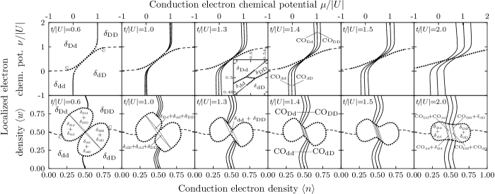
Figure 1: Evolution of the cross-sections of the global phase diagram under $t$ increase for $|U|=1$, in terms of the chemical potentials (upper panels) and densities (lower panels) of the localized and conduction electrons. In phase subscripts throughout this paper, the first and second subscripts respectively describe localized and conduction electron densities, as dilute (d) or dense (D). The dotted and thick full lines are respectively first- and second-order phase transitions. Phase separation, i.e., phase coexistence occurs inside the dotted boundaries, as identified appropriately but not repeatedly in the figure. The dashed lines are not phase transitions, but smooth changes between the different density regions of the disordered ($\delta$) phase. The charge-ordered phases are denoted by CO. The charge-ordered phases occur as strips near the half filling of the conduction electrons. Phase separation occurs near the simultaneous half filling of both the localized and conduction electrons. The four rounded coexistence regions, two of which disappear as $t$ is increased, are two-phase coexistence regions between the disordered $\delta$ phases that are distinguished by electron densities. The narrow triangular regions are three-phase coexistence regions between the $\delta$ phases. The second-order transition lines bounding the charge-ordered CO phases terminate at critical endpoints on the coexistence regions. These endpoints, as $t$ is increased, move past each other, as detailed in Sec.IV below, leading to coexistence regions between the different charge-ordered phases and between the charge-ordered and disordered phases.

The Falicov-Kimball model (FKM) was first proposed by L. M. Falicov and Kimball Falicov to analyze the thermodynamics of semiconductor-metal transitions in SmB₆ and transition-metal oxides RamirezFalicov70 ; RamirezFalicov71 ; Plischke ; GoncalvesDaSilva . The model incorporates two types of electrons: one type can undergo hopping between sites and the other type cannot hop, thereby being localized at the sites. Thus, in its introduction, FKM described the Coulomb interaction between mobile $d$ band electrons and localized $f$ band electrons. There have been a multitude of subsequent physical interpretations based on this interaction, including that of localized ions attractively interacting with mobile electrons, which yields crystalline formation Kennedy ; Lieb . Another physical interpretation of the model is as a binary alloy, in which the localized degree of freedom reflects A or B atom occupation FreericksFalicov ; Freericks . In this paper we employ the original language, with $d$ and $f$ electrons as conduction and localized electrons with a repulsive interaction between them.

Since there is no interacting spin degree of freedom in the Hamiltonian, the model is traditionally studied in the spinless case, commonly referred as the spinless FKM (SFKM) and which is in fact a special case of the Hubbard model in which one type of spin (e.g., spin-up) cannot hop Hubbard . In spite of its simplicity, this model is able to describe many physical phenomena in rare-earth and transition metal compounds, such as metal transitions, charge ordering, etc.

Beyond the introduction of the spin degree of freedom for both electrons Brandt ; Farkasovsky99 ; Zlatic ; Minh-Tien ; Lemanski ; Farkasovsky05 ; BrydonGulacsi06a ; ZlaticFreericks01a ; ZlaticFreericks01b ; ZlaticFreericks03 ; MillerFreericks01 ; FreericksNikolic01 ; FreericksNikolic02 ; AllubAlascio96 ; AllubAlascio97 ; LetfulovFreericks01 ; Ramakrishnan03 , there also exist many extensions of the original model. The most widely studied extensions include multiband hybridization Lawrence ; Leder ; Hanke ; Baeck ; LiuHo83 ; LiuHo84 ; Portengen96 ; BrydonGulacsi06b , $f-f$ hopping Kotecky ; Batista ; Yin03 ; Batista04 ; Ueltschi , correlated hopping Michielsen ; Tranh-Hai ; Gajek ; Wojtkiewicz01 ; CencarikovaFarkasovsky04 , non-bipartite lattices CencarikovaFarkasovsky07 ; GruberMacris97 , hard-core bosonic particles GruberMacris97 , magnetic fields ZlaticFreericks01b ; AllubAlascio96 ; AllubAlascio97 ; LetfulovFreericks01 ; Ramakrishnan03 ; GruberMacris97 ; FreericksZlatic98 , and next-nearest-neighbor hopping Wojtkiewicz06 . Exhaustive reviews are available in Refs. FreericksZlatic03 ; Jedrzejewski ; GruberMacris96 ; GruberUeltschi . The wider physical application of both the basic FKM and its extended versions have aimed at explaining valence transitions Farkasovsky99 ; ZlaticFreericks01a ; ZlaticFreericks01b ; ZlaticFreericks03 , metal-insulator transitions Farkasovsky99 ; MillerFreericks01 ; FreericksNikolic01 ; FreericksNikolic02 ; FreericksNikolic03 , mixed valence phenomena SubrahmanyamBarma88 , Raman scattering FreericksDevereaux01 , colossal magnetoresistance AllubAlascio96 ; AllubAlascio97 ; LetfulovFreericks01 ; Ramakrishnan03 , electronic ferroelectricity Batista ; Batista04 ; Portengen96 ; Yin03 , and phase separation Farkasovsky99 ; Ueltschi ; Michielsen ; Freericks96 ; Freericks02a ; Freericks02b .

After the initial works on the FKM Falicov ; RamirezFalicov70 ; RamirezFalicov71 ; Plischke ; GoncalvesDaSilva , the literature had to wait 14 years for the celebrated first rigorous results. Two independent studies, by Kennedy and Lieb Kennedy ; Lieb and by Brandt and Schmidt BrandtSchmidt86 ; BrandtSchmidt87 , proved for dimensions $d\geq 2$ that, at low temperatures, FKM has long-range charge order with the formation of two sublattices. Various methods have been used in the study of the FKM. In most of these studies, either the $d\rightarrow\infty$ infinite-dimensional limit or $d=1,2$ low-dimensional cases have been investigated. Studies include limiting cases such as ground-state analysis or the large interaction limit. Renormalization-group theory Wilson offers fully physical and fairly easy techniques to yield global phase diagrams and other physical phenomena.

This non-trivial nature of SFKM motivated us to determine the global phase diagram of the model, which resulted in a richly complex phase diagram involving charge ordering and phase coexistence, as exemplified in Fig. 1.

We use the general method for arbitrary dimensional quantum systems developed by A. Falicov and Berker AFalicov to obtain the global phase diagram of the SFKM in $d=3$, in terms of both the chemical potentials and the densities of the two types of electrons, for all temperatures. The outline of this paper is as follows: In Sec.II, we introduce the SFKM and, in Sec.III, we present the method AFalicov . Calculated phase diagrams are presented in Sec.IV, for the non-hopping ($t=0$) classical submodel and for the hopping ($t\neq 0$) quantum regimes of small, intermediate, and large $|U|$. We conclude the paper in Sec.V.

II Spinless Falicov-Kimball Model

The SFKM is defined by the Hamiltonian

$$\begin{split}-\beta\mathcal{H}&=t\sum_{\langle ij\rangle}\left(c_{i}^{{\dagger}}c_{j}+c_{j}^{{\dagger}}c_{i}\right)+U_{0}\sum_{i}n_{i}w_{i}\\ &+\mu_{0}\sum_{i}n_{i}+\nu_{0}\sum_{i}w_{i}\>,\end{split}$$ (1)

where $\beta=1/k_{B}T$ and $\langle ij\rangle$ denotes that the sum runs over all nearest-neighbor pairs of sites. Note that, as in all renormalization-group studies, the Hamiltonian has absorbed the inverse temperature. The dimensionless hopping strength $t$ can therefore be used as the inverse temperature. Here $c_{i}^{{\dagger}}$ and $c_{i}$ are respectively creation and annihilation operators for the conduction electrons at lattice site $i$, obeying the anticommutation rules $\{c_{i},c_{j}\}=\{c_{i}^{{\dagger}},c_{j}^{{\dagger}}\}=0$ and $\{c_{i}^{{\dagger}},c_{j}\}=\delta_{ij}$, while $n_{i}=c_{i}^{{\dagger}}c_{i}$ and $w_{i}$ are electron number operators for conduction and localized electrons respectively. The operator $w_{i}$ takes the values $1$ or $0$, for site $i$ being respectively occupied or unoccupied by a localized electron. The particles are fermions, so that the Pauli exclusion principle forbids the occupation of a given site by more than one localized electron or by more than one conduction electron.

The first term of the Hamiltonian is the kinetic energy term, responsible for the quantum nature of the model. The system being invariant under sign change of $t$ (via a phase change of the local basis states in one sublattice), only positive $t$ values are considered. The second term is the screened on-site Coulomb interaction between localized and conduction electrons, with positive and negative $U_{0}$ values corresponding to attractive and repulsive interactions. We consider only the repulsive case, since the attractive case can be connected to the repulsive one by the particle-hole symmetry possessed by either type of electrons. Particle-hole symmetries are achieved by the transformations of $w_{i}\rightarrow 1-w_{i}$ for the localized electrons and $c_{i}^{{\dagger}}\rightarrow\kappa_{i}c_{i}$, $c_{i}\rightarrow\kappa_{i}c_{i}^{{\dagger}}$ for the conduction electrons, where, for a bipartite lattice, $\kappa_{i}=1$ for one sublattice and $\kappa_{i}=-1$ for the other FreericksFalicov ; GruberUeltschi . The last two terms of the Hamiltonian are the chemical potential terms with $\nu_{0}$ and $\mu_{0}$ being the chemical potential for a localized and conduction electron.

In order to carry out a renormalization-group transformation easily, we trivially rearrange the Hamiltonian given in Eq.(1) into the equivalent form of

$$\begin{split}-\beta\mathcal{H}=&\sum_{\langle ij\rangle}\bigg{[}t\left(c_{i}^{{\dagger}}c_{j}+c_{j}^{{\dagger}}c_{i}\right)+U\left(n_{i}w_{i}+n_{j}w_{j}\right)\\ &\qquad\quad\quad~{}~{}\,+\mu\left(n_{i}+n_{j}\right)+\nu\left(w_{i}+w_{j}\right)\bigg{]}\\ \equiv&\sum_{\langle ij\rangle}\left[-\beta\mathcal{H}_{i,j}\right],\end{split}$$ (2)

where, for a $d$-dimensional hypercubic lattice, $U=U_{0}/2d$, $\mu=\mu_{0}/2d$, $\nu=\nu_{0}/2d$, and $-\beta\mathcal{H}_{i,j}$ is the two-site Hamiltonian involving only nearest-neighbor sites $i$ and $j$.

III Renormalization-Group Theory

III.1 Suzuki-Takano Method in $d=1$

In $d=1$ the Hamiltonian in Eq.(2) is

$$-\beta\mathcal{H}=\sum_{i}\left[-\beta\mathcal{H}_{i,i+1}\right].$$ (3)

The renormalization-group procedure traces out half of the degrees of freedom in the partition function Suzuki ; Takano ,

$$\begin{split}\mbox{Tr}_{\mbox{\tiny odd}}e^{-\beta\mathcal{H}}=&\mbox{Tr}_{\mbox{\tiny odd}}e^{\sum_{i}\left[-\beta\mathcal{H}_{i,i+1}\right]}\\ =&\mbox{Tr}_{\mbox{\tiny odd}}e^{\sum_{i}^{\mbox{\tiny odd}}\left[-\beta\mathcal{H}_{i-1,i}-\beta\mathcal{H}_{i,i+1}\right]}\\ \simeq&\prod_{i}^{\mbox{\tiny odd}}\mbox{Tr}_{i}e^{\left[-\beta\mathcal{H}_{i-1,i}-\beta\mathcal{H}_{i,i+1}\right]}\\ =&\prod_{i}^{\mbox{\tiny odd}}e^{-\beta^{\prime}\mathcal{H}^{\prime}_{i-1,i+1}}\\ \simeq&e^{\sum_{i}^{\mbox{\tiny odd}}\left[-\beta^{\prime}\mathcal{H}^{\prime}_{i-1,i+1}\right]}=e^{-\beta^{\prime}\mathcal{H}^{\prime}}.\end{split}$$ (4)

Here and throughout this paper primes are used for the renormalized system. Thus, as an approximation, the non-commutativity of the operators beyond three consecutive sites is ignored at each successive length scale, in the two steps indicated by $\simeq$ in the above equation. Earlier studies AFalicov ; Suzuki ; Takano ; Tomczak ; TomczakRichter96 ; TomczakRichter03 ; Hinczewski05 ; Hinczewski06 ; Hinczewski08 ; Kaplan2 ; Kaplan ; Sariyer have established the quantitative validity of this procedure.

The above transformation is algebraically summarized in

$$e^{-\beta^{\prime}\mathcal{H}^{\prime}_{i,k}}=\mbox{Tr}_{\!\tiny j\,}e^{\left\{-\beta\mathcal{H}_{i,j}-\beta\mathcal{H}_{j,k}\right\}}\>,$$ (5)

where $i,j,k$ are three successive sites. The operator $-\beta^{\prime}\mathcal{H}^{\prime}_{i,k}$ acts on two-site states, while the operator $-\beta\mathcal{H}_{i,j}-\beta\mathcal{H}_{j,k}$ acts on three-site states. Thus we can rewrite Eq.(5) in matrix form as

$$\langle u_{i}v_{k}|e^{-\beta^{\prime}\mathcal{H}^{\prime}_{i,k}}|\bar{u}_{i}\bar{v}_{k}\rangle=\\ \sum_{s_{j}}\langle u_{i}\,s_{j}\,v_{k}|e^{-\beta\mathcal{H}_{i,j}-\beta\mathcal{H}_{j,k}}|\bar{u}_{i}\,s_{j}\,\bar{v}_{k}\rangle,$$ (6)

where state variables $u_{\ell}$, $v_{\ell}$, $s_{\ell}$, $\bar{u}_{\ell}$, and $\bar{v}_{\ell}$ can be one of the four possible single-site $|w_{\ell},n_{\ell}\rangle$ states at each site $\ell$, namely one of $|00\rangle$, $|01\rangle$, $|10\rangle$, and $|11\rangle$. Eq.(6) indicates that the unrenormalized $64\times 64$ matrix on the right-hand side is contracted into the renormalized $16\times 16$ matrix on the left-hand side. We use two-site basis states, $\{|\phi_{p}\rangle\}$, and three-site basis states, $\{|\psi_{q}\rangle\}$, in order to block-diagonalize the matrices in Eq.(6). These basis states are the eigenstates of total localized and conduction electron numbers. The set of $\{|\phi_{p}\rangle\}$ and $\{|\psi_{q}\rangle\}$ are given in Tables 1 and 2 respectively. The corresponding block-diagonal Hamiltonian matrices are given in Appendices A and B.

$w$	$n$	$u$	Two-site basis states
$0$	$0$	$+$	$|\phi_{1}\rangle=|00,00\rangle$
$0$	$1$	$+$	$|\phi_{2}\rangle=\frac{1}{\sqrt{2}}\{|00,01\rangle+|01,00\rangle\}$
$0$	$1$	$-$	$|\phi_{3}\rangle=\frac{1}{\sqrt{2}}\{|00,01\rangle-|01,00\rangle\}$
$0$	$2$	$-$	$|\phi_{4}\rangle=|01,01\rangle$
$1$	$0$	$+$	$|\phi_{5}\rangle=|00,10\rangle$
$1$	$1$	$+$	$|\phi_{6}\rangle=\frac{1}{\sqrt{2}}\{|00,11\rangle+|01,10\rangle\}$
$1$	$1$	$-$	$|\phi_{7}\rangle=\frac{1}{\sqrt{2}}\{|00,11\rangle-|01,10\rangle\}$
$1$	$2$	$-$	$|\phi_{8}\rangle=|01,11\rangle$
$2$	$0$	$+$	$|\phi_{13}\rangle=|10,10\rangle$
$2$	$1$	$+$	$|\phi_{14}\rangle=\frac{1}{\sqrt{2}}\{|10,11\rangle+|11,10\rangle\}$
$2$	$1$	$-$	$|\phi_{15}\rangle=\frac{1}{\sqrt{2}}\{|10,11\rangle-|11,10\rangle\}$
$2$	$2$	$-$	$|\phi_{16}\rangle=|11,11\rangle$

Table 1: The two-site basis states that appear in Eq.(7), in the form $|w_{i}n_{i},w_{j}n_{j}\rangle$. The total localized and conduction electron numbers $w$ and $n$, the eigenvalue $u$ of the operator $T_{ij}$ defined after Eq.(8) are indicated. $|\phi_{9-12}\rangle$ are respectively obtained from $|\phi_{5-8}\rangle$ by the action of $T_{ij}$, while the corresponding Hamiltonian matrix elements are multiplied by the $u$ values of the states.

$w$	$n$	$u$	Three-site basis states
$0$	$0$	$+$	$|\psi_{1}\rangle=|00,00,00\rangle$
$0$	$1$	$+$	$|\psi_{2}\rangle=\frac{1}{\sqrt{2}}\{|00,00,01\rangle+|01,00,00\rangle\}$
$0$	$1$	$+$	$|\psi_{3}\rangle=|00,01,00\rangle$
$0$	$1$	$-$	$|\psi_{4}\rangle=\frac{1}{\sqrt{2}}\{|00,00,01\rangle-|01,00,00\rangle\}$
$0$	$2$	$+$	$|\psi_{5}\rangle=\frac{1}{\sqrt{2}}\{|00,01,01\rangle-|01,01,00\rangle\}$
$0$	$2$	$-$	$|\psi_{6}\rangle=|01,00,01\rangle$
$0$	$2$	$-$	$|\psi_{7}\rangle=\frac{1}{\sqrt{2}}\{|00,01,01\rangle+|01,01,00\rangle\}$
$0$	$3$	$-$	$|\psi_{8}\rangle=|01,01,01\rangle$
$1$	$0$	$+$	$|\psi_{9}\rangle=|00,00,10\rangle$
$1$	$0$	$+$	$|\psi_{10}\rangle=|00,10,00\rangle$
$1$	$1$	$+$	$|\psi_{12}\rangle=\frac{1}{\sqrt{2}}\{|00,00,11\rangle+|01,00,10\rangle\}$
$1$	$1$	$+$	$|\psi_{13}\rangle=\frac{1}{\sqrt{2}}\{|00,10,01\rangle+|01,10,00\rangle\}$
$1$	$1$	$+$	$|\psi_{15}\rangle=|00,01,10\rangle$
$1$	$1$	$+$	$|\psi_{16}\rangle=|00,11,00\rangle$
$1$	$1$	$-$	$|\psi_{18}\rangle=\frac{1}{\sqrt{2}}\{|00,00,11\rangle-|01,00,10\rangle\}$
$1$	$1$	$-$	$|\psi_{19}\rangle=\frac{1}{\sqrt{2}}\{|00,10,01\rangle-|01,10,00\rangle\}$
$1$	$2$	$+$	$|\psi_{21}\rangle=\frac{1}{\sqrt{2}}\{|00,01,11\rangle-|01,01,10\rangle\}$
$1$	$2$	$+$	$|\psi_{22}\rangle=\frac{1}{\sqrt{2}}\{|00,11,01\rangle-|01,11,00\rangle\}$
$1$	$2$	$-$	$|\psi_{24}\rangle=|01,00,11\rangle$
$1$	$2$	$-$	$|\psi_{25}\rangle=|01,10,01\rangle$
$1$	$2$	$-$	$|\psi_{27}\rangle=\frac{1}{\sqrt{2}}\{|00,01,11\rangle+|01,01,10\rangle\}$
$1$	$2$	$-$	$|\psi_{28}\rangle=\frac{1}{\sqrt{2}}\{|00,11,01\rangle+|01,11,00\rangle\}$
$1$	$3$	$-$	$|\psi_{30}\rangle=|01,01,11\rangle$
$1$	$3$	$-$	$|\psi_{31}\rangle=|01,11,01\rangle$
$2$	$0$	$+$	$|\psi_{33}\rangle=|00,10,10\rangle$
$2$	$0$	$+$	$|\psi_{34}\rangle=|10,00,10\rangle$
$2$	$1$	$+$	$|\psi_{36}\rangle=\frac{1}{\sqrt{2}}\{|00,10,11\rangle+|01,10,10\rangle\}$
$2$	$1$	$+$	$|\psi_{37}\rangle=\frac{1}{\sqrt{2}}\{|10,00,11\rangle+|11,00,10\rangle\}$
$2$	$1$	$+$	$|\psi_{39}\rangle=|00,11,10\rangle$
$2$	$1$	$+$	$|\psi_{40}\rangle=|10,01,10\rangle$
$2$	$1$	$-$	$|\psi_{42}\rangle=\frac{1}{\sqrt{2}}\{|00,10,11\rangle-|01,10,10\rangle\}$
$2$	$1$	$-$	$|\psi_{43}\rangle=\frac{1}{\sqrt{2}}\{|10,00,11\rangle-|11,00,10\rangle\}$
$2$	$2$	$+$	$|\psi_{45}\rangle=\frac{1}{\sqrt{2}}\{|00,11,11\rangle-|01,11,10\rangle\}$
$2$	$2$	$+$	$|\psi_{46}\rangle=\frac{1}{\sqrt{2}}\{|10,01,11\rangle-|11,01,10\rangle\}$
$2$	$2$	$-$	$|\psi_{48}\rangle=|01,10,11\rangle$
$2$	$2$	$-$	$|\psi_{49}\rangle=|11,00,11\rangle$
$2$	$2$	$-$	$|\psi_{51}\rangle=\frac{1}{\sqrt{2}}\{|00,11,11\rangle+|01,11,10\rangle\}$
$2$	$2$	$-$	$|\psi_{52}\rangle=\frac{1}{\sqrt{2}}\{|10,01,11\rangle+|11,01,10\rangle\}$
$2$	$3$	$-$	$|\psi_{54}\rangle=|01,11,11\rangle$
$2$	$3$	$-$	$|\psi_{55}\rangle=|11,01,11\rangle$
$3$	$0$	$+$	$|\psi_{57}\rangle=|10,10,10\rangle$
$3$	$1$	$+$	$|\psi_{58}\rangle=\frac{1}{\sqrt{2}}\{|10,10,11\rangle+|11,10,10\rangle\}$
$3$	$1$	$+$	$|\psi_{59}\rangle=|10,11,10\rangle$
$3$	$1$	$-$	$|\psi_{60}\rangle=\frac{1}{\sqrt{2}}\{|10,10,11\rangle-|11,10,10\rangle\}$
$3$	$2$	$+$	$|\psi_{61}\rangle=\frac{1}{\sqrt{2}}\{|10,11,11\rangle-|11,11,10\rangle\}$
$3$	$2$	$-$	$|\psi_{62}\rangle=|11,10,11\rangle$
$3$	$2$	$-$	$|\psi_{63}\rangle=\frac{1}{\sqrt{2}}\{|10,11,11\rangle+|11,11,10\rangle\}$
$3$	$3$	$-$	$|\psi_{64}\rangle=|11,11,11\rangle$

Table 2: The three-site basis states that appear in Eq.(7), in the form $|w_{i}n_{i},w_{j}n_{j},w_{k}n_{k}\rangle$. The total localized and conduction electron numbers $w$ and $n$, the eigenvalue $u$ of the operator $T_{ik}$ defined after Eq.(8) are indicated. $\{|\psi_{11+3x}\rangle\}$, $x=0,1,\ldots,15$, are respectively obtained from $\{|\psi_{9+3x}\rangle\}$ by the action of $T_{ik}$, while the corresponding Hamiltonian matrix elements are multiplied by the $u$ values of the states.

Phase	The interaction constants $K_{\alpha}$ at the phase sinks
sink	$t$	$U$	$\mu$	$\nu$	$J$	$K$	$L$	$P$	$V_{n}$	$V_{w}$	$Q$	$R$
$\delta_{\textrm{dd}}$	$0$	$0$	$-\infty$	$-\infty$	$0$	$0$	$0$	$0$	$0$	$0$	$0$	$0$
$\delta_{\textrm{dD}}$	$0$	$\infty$	$\infty$	$-\infty$	$0$	$0$	$0$	$0$	$0$	$0$	$0$	$0$
$\delta_{\textrm{Dd}}$	$0$	$\infty$	$-\infty$	$\infty$	$0$	$0$	$0$	$0$	$0$	$0$	$0$	$0$
$\delta_{\textrm{DD}}$	$0$	$0$	$\infty$	$\infty$	$0$	$0$	$0$	$0$	$0$	$0$	$0$	$0$
CO${}_{\textrm{dd}}$	$\infty$	$\infty$	$-\infty$	$-\infty$	$\infty$	$-\infty$	$\infty$	$-\infty$	$-\infty$	$\infty$	$\infty$	$-\infty$
CO${}_{\textrm{dD}}$	$\infty$	$\infty$	$\infty$	$-\infty$	$\infty$	$-\infty$	$\infty$	$\infty$	$-\infty$	$\infty$	$\infty$	$\infty$
CO${}_{\textrm{Dd}}$	$\infty$	$\infty$	$-\infty$	$\infty$	$\sim 50$	$-\infty$	$\infty$	$-\infty$	$\sim-20$	$\infty$	$\infty$	$-\infty$
CO${}_{\textrm{DD}}$	$\infty$	$\infty$	$\infty$	$\infty$	$\sim 140$	$-\infty$	$\infty$	$\infty$	$\sim-40$	$\infty$	$\infty$	$\infty$

Phase	The runaway coefficients $K_{\alpha}^{\prime}/K_{\alpha}$ at the phase sinks
sink	$t^{\prime}/t$	$U^{\prime}/U$	$\mu^{\prime}/\mu$	$\nu^{\prime}/\nu$	$J^{\prime}/J$	$K^{\prime}/K$	$L^{\prime}/L$	$P^{\prime}/P$	$V_{n}^{\prime}/V_{n}$	$V_{w}^{\prime}/V_{w}$	$Q^{\prime}/Q$	$R^{\prime}/R$
$\delta_{\textrm{dd}}$, $\delta_{\textrm{DD}}$	$-$	$-$	$4$	$4$	$-$	$-$	$-$	$-$	$-$	$-$	$-$	$-$
$\delta_{\textrm{dD}}$, $\delta_{\textrm{Dd}}$	$-$	$4$	$4$	$4$	$-$	$-$	$-$	$-$	$-$	$-$	$-$	$-$
CO${}_{\textrm{dd}}$, CO${}_{\textrm{dD}}$	$2$	$2$	$2$	$4$	$4/3$	$2$	$4/3$	$2$	$4/3$	$2$	$2$	$2$
CO${}_{\textrm{Dd}}$, CO${}_{\textrm{DD}}$	$2$	$2$	$2$	$4$	$1$	$2$	$4/3$	$2$	$1$	$2$	$2$	$2$

Phase	The expectation values $M_{\alpha}$ at the phase sinks												Character
sink	$\langle\hat{t}\rangle$	$\langle\hat{U}\rangle$	$\langle\hat{\mu}\rangle$	$\langle\hat{\nu}\rangle$	$\langle\hat{J}\rangle$	$\langle\hat{K}\rangle$	$\langle\hat{L}\rangle$	$\langle\hat{P}\rangle$	$\langle\hat{V_{n}}\rangle$	$\langle\hat{V_{w}}\rangle$	$\langle\hat{Q}\rangle$	$\langle\hat{R}\rangle$
$\delta_{\textrm{dd}}$	$0$	$0$	$0$	$0$	$0$	$0$	$0$	$0$	$0$	$0$	$0$	$0$	dilute - dilute
$\delta_{\textrm{dD}}$	$0$	$0$	$2$	$0$	$1$	$0$	$0$	$0$	$0$	$0$	$0$	$0$	dilute - dense
$\delta_{\textrm{Dd}}$	$0$	$0$	$0$	$2$	$0$	$1$	$0$	$0$	$0$	$0$	$1$	$2$	dense - dilute
$\delta_{\textrm{DD}}$	$0$	$2$	$2$	$2$	$1$	$1$	$1$	$2$	$2$	$2$	$-1$	$-2$	dense - dense
CO${}_{\textrm{dd}}$	$-a$	$0$	$a$	$0$	$0$	$0$	$0$	$0$	$0$	$0$	$0$	$0$	dilute - charge ord. dilute
CO${}_{\textrm{dD}}$	$-a$	$0$	$2-a$	$0$	$1-a$	$0$	$0$	$0$	$0$	$0$	$0$	$0$	dilute - charge ord. dense
CO${}_{\textrm{Dd}}$	$-a$	$a$	$a$	$2$	$0$	$1$	$0$	$a$	$0$	$a$	$1$	$2$	dense - charge ord. dilute
CO${}_{\textrm{DD}}$	$-a$	$2-a$	$2-a$	$2$	$1-a$	$1$	$1-a$	$2-a$	$2-2a$	$2-a$	$-1+2a$	$-2+4a$	dense - charge ord. dense

Table 3: Interaction constants $K_{\alpha}$, runaway coefficients $K_{\alpha}^{\prime}/K_{\alpha}$, and expectation values $M_{\alpha}=\langle\hat{K_{\alpha}}\rangle$, at the phase sinks. Here, $\hat{K_{\alpha}}$ are used as abbreviations for the conjugate operators for interaction constants $K_{\alpha}$, e.g., $\langle\hat{t}\rangle=\langle c_{i}^{{\dagger}}c_{j}+c_{j}^{{\dagger}}c_{i}\rangle$, $\langle\hat{U}\rangle=\langle n_{i}w_{i}+n_{j}w_{j}\rangle$, etc. The non-zero hopping expectation value is $-a=-0.629050$. In the subscripts in the first columns, the left and right entries refer to the localized and conduction electrons, respectively, as dilute (d) or dense (D).

Phase

Boundary

Interaction constants $K_{\alpha}$ at the boundary fixed points

Relevant

eigenvalue

boundary

type

$t$

$U$

$\mu$

$\nu$

$J$

$K$

$L$

$P$

$V_{n}$

$V_{w}$

$Q$

$R$

exponent $y_{1}$

CO${}_{\textrm{dD}}$/CO${}_{\textrm{Dd}}$

1st

$\infty$

$-\infty$

$\infty$

$-\infty$

$\infty$

$\infty$

$\infty$

$-\infty$

$-\infty$

$\infty$

$\infty$

$-\infty$

$2\mu-2\nu+J-K$

3

order

$-Q-2R=0$

CO${}_{\textrm{dd}}$/$\delta_{\textrm{dd}}$

2nd

$\infty$

$\infty$

$-\infty$

$-\infty$

$\infty$

$-\infty$

$\infty$

$-\infty$

$-\infty$

$\infty$

$\infty$

$-\infty$

$t+\mu=1.744253$

0.273873

order

CO${}_{\textrm{dD}}$/$\delta_{\textrm{dD}}$

2nd

$\infty$

$\infty$

$\infty$

$-\infty$

$\infty$

$-\infty$

$\infty$

$-\infty$

$\infty$

$\infty$

$\infty$

$-\infty$

$t-\mu-J=1.744253$

0.273873

order

CO${}_{\textrm{Dd}}$/$\delta_{\textrm{Dd}}$

2nd

$\infty$

$\infty$

$-\infty$

$\infty$

$\infty$

$-\infty$

$\infty$

$-\infty$

$-\infty$

$\infty$

$\infty$

$-\infty$

$t+U+\mu+P+V_{w}$

0.273873

order

$=1.744253$

CO${}_{\textrm{DD}}$/$\delta_{\textrm{DD}}$

2nd

$\infty$

$\infty$

$\infty$

$\infty$

$\infty$

$-\infty$

$\infty$

$\infty$

$-\infty$

$\infty$

$\infty$

$\infty$

$t-U-\mu-J-L-P$

0.273873

order

$-2V_{n}-V_{w}+2Q+4R=0$

CO${}_{\textrm{dd}}$/CO${}_{\textrm{dD}}$

2nd

$\infty$

$\infty$

$-\infty$

$-\infty$

$\infty$

$-\infty$

$\infty$

$-\infty$

$-\infty$

$\infty$

$\infty$

$-\infty$

$2\mu+J=0$

1.420396

order

CO${}_{\textrm{Dd}}$/CO${}_{\textrm{DD}}$

2nd

$\infty$

$\infty$

$-\infty$

$\infty$

$\infty$

$-\infty$

$\infty$

$-\infty$

$\infty$

$\infty$

$\infty$

$-\infty$

$2U+2\mu+J+L+2P$

1.420396

order

$+2V_{n}+2V_{w}-2Q-4R=0$

Table 4: Interaction constants $K_{\alpha}$ and relevant eigenvalue exponents $y_{1}$ at the phase boundary fixed points. For first-order phase transitions, $y_{1}=d=3$.

With these basis states, Eq.(6) can be rewritten as

$$\langle\phi_{p}|e^{-\beta^{\prime}\mathcal{H}^{\prime}_{i,k}}|\phi_{\bar{p}}\rangle=\sum_{\begin{subarray}{c}u,v,\\ \bar{u},\bar{v},s\end{subarray}}\sum_{\begin{subarray}{c}q,\bar{q}\end{subarray}}\langle\phi_{p}|u_{i}v_{k}\rangle\langle u_{i}s_{j}v_{k}|\psi_{q}\rangle\cdot\\ \langle\psi_{q}|e^{-\beta\mathcal{H}_{i,j}-\beta\mathcal{H}_{j,k}}|\psi_{\bar{q}}\rangle\langle\psi_{\bar{q}}|\bar{u}_{i}s_{j}\bar{v}_{k}\rangle\langle\bar{u}_{i}\bar{v}_{k}|\phi_{\bar{p}}\rangle.$$ (7)

Once written in the basis states $\{|\phi_{p}\rangle\}$, the block-diagonal renormalized matrix has 13 independent elements, which means that renormalization-group transformation of the Hamiltonian generates 9 more interaction constants apart from $t$, $U$, $\mu$, and $\nu$. In this 13-dimensional interaction space, the form of the Hamiltonian stays closed under renormalization-group transformations. This Hamiltonian is

$$\begin{split}-\beta\mathcal{H}_{i,j}&=t\left(c_{i}^{{\dagger}}c_{j}+c_{j}^{{\dagger}}c_{i}\right)+U\left(n_{i}w_{i}+n_{j}w_{j}\right)\\ &+\mu\left(n_{i}+n_{j}\right)+\nu\left(w_{i}+w_{j}\right)+Jn_{i}n_{j}\\ &+Kw_{i}w_{j}+Ln_{i}n_{j}w_{i}w_{j}+P\left(n_{i}w_{j}+n_{j}w_{i}\right)\\ &+V_{n}n_{i}n_{j}(w_{i}+w_{j})+V_{w}(n_{i}+n_{j})w_{i}w_{j}\\ &+QT_{ij}w_{i}w_{j}+RT_{ij}(w_{i}+w_{j})+G,\end{split}$$ (8)

where $T_{ij}$ is a local operator that switches the conduction electron states of sites $i$ and $j$: $T_{ij}|w_{i}n_{i},w_{j}n_{j}\rangle=u|w_{i}n_{j},w_{j}n_{i}\rangle$ with $u=1$ for $n_{i}+n_{j}<2$ and $u=-1$ otherwise. When $T_{ik}$ is applied, further below, to three consecutive sites $i$, $j$, $k$, $T_{ik}|w_{i}n_{i},w_{j}n_{j},w_{k}n_{k}\rangle=u|w_{i}n_{k},w_{j}n_{j},w_{k}n_{i}\rangle$ with $u=1$ for $n_{i}+n_{j}+n_{k}<2$ and $u=-1$ otherwise.

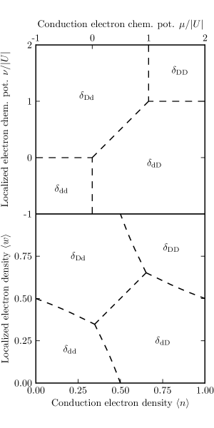
Figure 2: Renormalization-group flow basins of the $t=0$ classical submodel, in the chemical potentials (upper panel) and densities (lower panel) of the localized and conduction electrons. In phase subscripts throughout this paper, the first and second subscripts respectively describe localized and conduction electron densities, as dilute (d) or dense (D). The dashed lines are not phase transitions, but smooth changes between the four different density regions of the disordered ($\delta$) phase.

To extract the renormalization-group recursion relations, we consider the matrix elements $\gamma_{p,\bar{p}}\equiv\langle\phi_{p}|e^{-\beta^{\prime}\mathcal{H}^{\prime}_{i,k}}|\phi_{\bar{p}}\rangle$. With $\gamma_{9,9}=\gamma_{5,5}$, $\gamma_{10,10}=\gamma_{6,6}$, $\gamma_{11,11}=\gamma_{7,7}$, and $\gamma_{12,12}=\gamma_{8,8}$, 12 out of 16 diagonal elements are independent and, with $\gamma_{10,11}=\gamma_{11,10}=-\gamma_{7,6}=-\gamma_{6,7}$, only one of the 4 off-diagonal elements is independent, summing up to 13 independent matrix elements. Thus we obtain the renormalized interaction constants in terms of $\{\gamma\}$, defining $\gamma_{p}\equiv\gamma_{p,p}$ for the diagonal elements and $\gamma_{0}\equiv\gamma_{6,7}$ for the only independent off-diagonal element:

$$t^{\prime}=\frac{1}{2}\ln\frac{\gamma_{2}}{\gamma_{3}},\quad U^{\prime}=\ln\frac{\gamma_{1}\gamma_{6}\gamma_{0}}{\gamma_{2}\gamma_{5}},\quad\mu^{\prime}=\frac{1}{2}\ln\frac{\gamma_{2}\gamma_{3}}{\gamma_{1}^{2}},\\ \nu^{\prime}=\frac{1}{2}\ln\frac{\gamma_{2}\gamma_{5}^{2}\gamma_{7}}{\gamma_{1}^{2}\gamma_{3}\gamma_{6}},\quad J^{\prime}=\ln\frac{\gamma_{1}\gamma_{4}}{\gamma_{2}\gamma_{3}},\\ K^{\prime}=\frac{1}{2}\ln\frac{\gamma_{1}^{2}\gamma_{3}\gamma_{6}^{2}\gamma_{13}^{2}\gamma_{15}}{\gamma_{2}\gamma_{5}^{4}\gamma_{7}^{2}\gamma_{14}},\quad L^{\prime}=\ln\frac{\gamma_{1}\gamma_{4}\gamma_{6}^{2}\gamma_{7}^{2}\gamma_{13}\gamma_{16}}{\gamma_{2}\gamma_{3}\gamma_{5}^{2}\gamma_{8}^{2}\gamma_{14}\gamma_{15}},\\ P^{\prime}=\ln\frac{\gamma_{1}\gamma_{6}}{\gamma_{2}\gamma_{5}\gamma_{0}},\quad V_{n}^{\prime}=\ln\frac{\gamma_{2}\gamma_{3}\gamma_{5}\gamma_{8}}{\gamma_{1}\gamma_{4}\gamma_{6}\gamma_{7}},\quad V_{w}^{\prime}=\ln\frac{\gamma_{2}\gamma_{5}^{2}\gamma_{14}}{\gamma_{1}\gamma_{6}^{2}\gamma_{13}},\\ Q^{\prime}=\frac{1}{2}\ln\frac{\gamma_{2}\gamma_{7}^{2}\gamma_{14}}{\gamma_{3}\gamma_{6}^{2}\gamma_{15}},\quad R^{\prime}=\frac{1}{2}\ln\frac{\gamma_{3}\gamma_{6}}{\gamma_{2}\gamma_{7}},\quad G^{\prime}=\ln\gamma_{1}.$$ (9)

The matrix elements $\{\gamma\}$ of the exponentiated renormalized Hamiltonian are connected, by Eq.(7), to the matrix elements, $\eta_{q,\bar{q}}\equiv\langle\psi_{q}|e^{-\beta\mathcal{H}_{i,j}-\beta\mathcal{H}_{j,k}}|\psi_{\bar{q}}\rangle$ of the exponentiated unrenormalized Hamiltonian,

$$\begin{split}\gamma_{0}=&\eta_{12,18}+\eta_{21,27}+\eta_{36,42}+\eta_{45,51},\\ \gamma_{1}=&\eta_{1}+\eta_{3}+\eta_{10}+\eta_{16},\\ \gamma_{2}=&\eta_{3}+\eta_{7}+\eta_{13}+\eta_{28},\\ \gamma_{3}=&\eta_{4}+\eta_{5}+\eta_{19}+\eta_{22},\\ \gamma_{4}=&\eta_{6}+\eta_{8}+\eta_{25}+\eta_{31},\\ \gamma_{5}=&\eta_{9}+\eta_{15}+\eta_{33}+\eta_{39},\\ \gamma_{6}=&\eta_{12}+\eta_{27}+\eta_{36}+\eta_{51},\\ \gamma_{7}=&\eta_{18}+\eta_{21}+\eta_{42}+\eta_{45},\\ \gamma_{8}=&\eta_{24}+\eta_{30}+\eta_{48}+\eta_{54},\\ \gamma_{13}=&\eta_{34}+\eta_{40}+\eta_{57}+\eta_{59},\\ \gamma_{14}=&\eta_{37}+\eta_{52}+\eta_{58}+\eta_{63},\\ \gamma_{15}=&\eta_{43}+\eta_{46}+\eta_{60}+\eta_{61},\\ \gamma_{16}=&\eta_{49}+\eta_{55}+\eta_{62}+\eta_{64}.\end{split}$$ (10)

The matrix elements $\eta_{q,\bar{q}}$ can be obtained in terms of the unrenormalized interactions via exponentiating the unrenormalized Hamiltonian matrix whose elements are given in Appendix B.

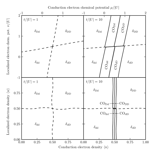
Figure 3: Constant $t/|U|$ cross-sections of the phase diagram for interaction $|U|=0.1$, in terms of the chemical potentials (upper panels) and densities (lower panels) of the localized and conduction electrons. In phase subscripts throughout this paper, the first and second subscripts respectively describe localized and conduction electron densities, as dilute (d) or dense (D). The full lines are second-order phase transitions. The dashed lines are not phase transitions, but smooth changes between the different density regions of the disordered ($\delta$) phase. The charge-ordered phases are denoted by CO. Details are shown in Fig. 4. Thus, for low values of the interaction, all phase boundaries are second order and there is no phase coexistence.

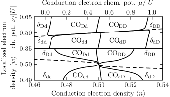
Figure 4: Zoomed portion of Fig. 3, for the $|U|=0.1$, $t/|U|=10$ phase diagram.

III.2 Renormalization-Group Transformation in $d>1$

Equations (9) and (10), together with Appendix B, constitute the renormalization-group recursion relations for $d=1$, in the form $\vec{K}^{\prime}=R(\vec{K})$, where $\vec{K}=(t,U,\mu,\nu,J,K,L,P,V_{n},V_{w},Q,R,G)$. To generalize to higher dimension $d>1$, we use the Migdal-Kadanoff procedure Migdal ; Kadanoff ,

$$\vec{K}^{\prime}=b^{d-1}R(\vec{K}),$$ (11)

where $b=2$ is the rescaling factor and $R$ is the renormalization-group transformation in $d=1$ for the interaction constants vector $\vec{K}$. This procedure is exact for $d$-dimensional hierarchical lattices BerkerOslund79 ; Kaufman81 ; Kaufman84 and a very good approximation for hypercubic lattices for obtaining complex phase diagrams.

Each phase in the phase diagram has its own (stable) fixed point(s), which is called a phase sink (Table 3). All points within a phase flow to the sink(s) of that phase under successive renormalization-group transformations. Phase boundaries also have their own (unstable) fixed points (Table 4), where the relevant exponent analysis gives the order of the phase transition. Thus, the repartition of the renormalization-group flows determine the phase diagram in thermodynamic-field space. Matrix multiplications, along the renormalization-group trajectory, with the derivative matrix of the recursion relations relate the expectation values at the starting point of the trajectory to the expectations values at the phase sink. The latter are determined (Table III) by the left eigenvector, with eigenvalue $b^{d}$, of the recursion matrix at the sink, where $b=2$ is the length-rescaling factor of the renormalization-group transformation. When the expectation values are thus calculated for the points of the phase boundary, the phase diagram in density space is determined.McKay84 ; Hinczewski06b

IV Global Phase Diagram of SFKM

The global phase diagram of SFKM is calculated, as described above, for the whole range of the interactions ($t$, $U$, $\nu$, $\mu$). The global phase diagram is thus 4-dimensional. $1/t$ can be taken as the temperature variable. We present the calculated global phase diagram in four subsections: The first subsection gives the $t=0$ classical submodel. The other subsections are devoted to small, intermediate, and large values of the interaction $|U|$. We present constant $t/|U|$ cross sections in terms of the localized and conduction electron chemical potentials $\nu/|U|$ and $\mu/|U|$and in terms of the localized and conduction electron densities $\langle w_{i}\rangle$ and $\langle n_{i}\rangle$.

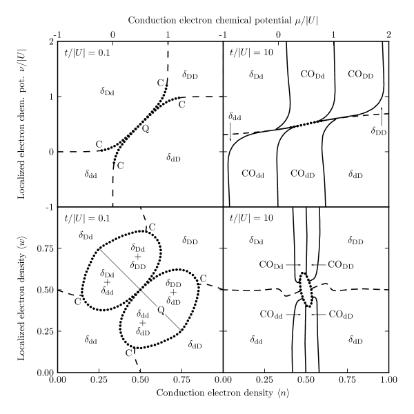
Figure 5: Constant $t/|U|$ cross-sections of the phase diagram for interaction $|U|=1$, in terms of the chemical potentials (upper panels) and densities (lower panels) of the localized and conduction electrons. The dotted and thick full lines are respectively first- and second-order phase transitions. Phase separation, i.e., phase coexistence occurs inside the dotted boundaries, as identified in the figure. The details of the coexistence region in the lower-right panel are given in Fig. 6. The quadruple point Q tie line is shown as the thin straight line. The dashed lines are not phase transitions, but smooth changes between the different density regions of the disordered ($\delta$) phase.

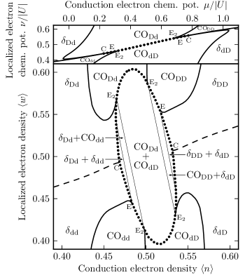
Figure 6: Zoomed portion of Fig. 5, for the $|U|=1$, $t/|U|=10$ phase diagram. The coexistence tie lines of the critical endpoints E and of the double critical endpoints E₂ are shown. Inside each region delimited by dotted lines and the endpoint tie lines, phase separation, i.e., phase coexistence occurs between phases as identified on this figure.

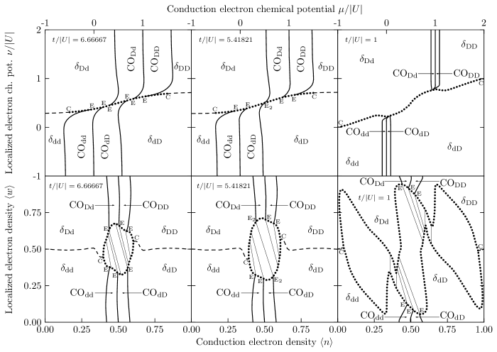
Figure 7: Constant $t/|U|$ cross-sections of the phase diagram for interactions $|U|=1.5,1.845628,10$ (left to right), in terms of the chemical potentials (upper panels) and densities (lower panels) of the localized and conduction electrons. The dotted and thick full lines are respectively first- and second-order phase transitions. The tie lines of the critical endpoints E and of the double critical endpoints E₂ are shown by thin straight lines. Phase separation, i.e., phase coexistence occurs within the regions bounded by the dotted lines and these endpoint tie lines, this coexistence being between the phases seen on each side of the dotted lines. In the upper-right chemical-potential panel, the first-order phase boundary exhibits, from the left to right, a sequence of the maximum, minimum, maximum, minimum points; the four corresponding tie lines are also shown in the lower-right density panel. These tie lines abut, on one end, very near maxima and minima of the lower and upper branches of the coexistence boundaries. The dashed lines are not phase transitions, but smooth changes between the different density regions of the $\delta$ phase.

IV.1 The Classical Submodel $t=0$

Setting the quantum effect to zero, $t=0$, yields the classical submodel, closed under the renormalization-group flows. The global flow basins in $\nu/|U|$ and $\mu/|U|$ are the same for all $U$, given in Fig. 2. There exist four regions of a disordered phase within this submodel, which are localized-dilute-conduction-dilute, localized-dilute-conduction-dense, localized-dense-conduction-dilute, and localized-dense-conduction-dense regions, denoted by $\delta_{\textrm{dd}}$, $\delta_{\textrm{dD}}$, $\delta_{\textrm{Dd}}$, and $\delta_{\textrm{DD}}$. [In phase subscripts throughout this paper, the first and second subscripts respectively describe localized and conduction electron densities, as dilute (d) or dense (D).] In the renormalization-group flows, each $\delta$ region is the basin of attraction of its own sink. The dashed lines between the different regions are not phase boundaries, but smooth transitions (such as the supercritical liquid - gas or up-magnetized - down-magnetized transitions), which are controlled by zero-coupling null fixed points.Berker0

It should be noted that the Suzuki-Takano and Migdal-Kadanoff methods are actually exact for this classical submodel, and yield exactly the same picture as obtained in Datta99 .

IV.2 The Small $|U|$ Regime

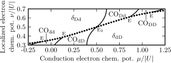
Figure 8: Zoomed portions of Fig. 7, for the $|U|=1.845628,t/|U|=5.41821$ phase diagram.

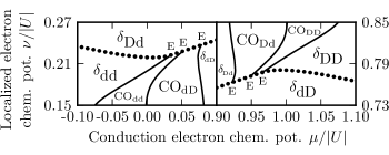
Figure 9: Two zoomed portions of Fig. 7, for the $|U|=10,t/|U|=1$ phase diagram.

In this subsection, we present our results for $|U|=0.1$, representative of the weak-interaction regime. The $t=0$ phase diagram of Fig. 2 evolves under the introduction of quantum effects via a non-zero hopping strength $t$. It should be noted that increasing the dimensionless Hamiltonian parameter $t$ is equivalent to reducing temperature, as in all renormalization-group studies. The first effect is the decrease and elimination (left panels of Fig. 3) of the (smooth) passage between the $\delta_{\textrm{Dd}}$ and $\delta_{\textrm{dD}}$ regions. With this elimination, all four regions meet at $\nu/|U|=\mu/|U|=0.5$ and $\langle w_{i}\rangle=\langle n_{i}\rangle=0.5$, the half filling of both localized and conduction electrons. With increasing $t$ (equivalent to decreasing temperature), four new, charge-ordered (CO) phases emerge at $t\simeq 0.6$. The CO phases occur at and near half filling of conduction electrons for the entire range of localized electron densities. The CO phases grow with increasing $t$ (decreasing temperature) until saturation at high $t$ (right panels of Fig. 3).

All of the new CO phases have non-zero hopping density $\langle c_{i}^{{\dagger}}c_{j}+c_{j}^{{\dagger}}c_{i}\rangle=-a=-0.629050$ at their phase sinks. The expectation values at the sinks are evaluated as the left eigenvector of the recursion matrix with eigenvalue $b^{d}$ McKay84 . In the CO phases, the hopping strength $t$ diverges to infinity under repeated renormalization-group transformations (whereas in the $\delta$ phases, $t$ vanishes under repeated renormalization-group transformations). The localized electron density is $\langle w_{i}+w_{j}\rangle=0$ at the sinks of CO${}_{\textrm{dd}}$ and CO${}_{\textrm{dD}}$, while $\langle w_{i}+w_{j}\rangle=2$ at the sinks of CO${}_{\textrm{Dd}}$ and CO${}_{\textrm{DD}}$, which throughout the corresponding phases calculationally translates McKay84 as low ($d$) and high ($D$) localized electron densities, respectively. Recall that on phase labels (CO and $\delta$) throughout this paper, the first and second subscripts respectively describe localized and conduction electron densities.

The conduction electron density is $\langle n_{i}+n_{j}\rangle=a=0.629050$ at the sinks of CO${}_{\textrm{dd}}$ and CO${}_{\textrm{Dd}}$, while $\langle n_{i}+n_{j}\rangle=2-a=1.370950$ at the sinks of CO${}_{\textrm{dD}}$ and CO${}_{\textrm{DD}}$. The nearest-neighbor conduction electron number correlation is $\langle n_{i}n_{j}\rangle=0$ at the sinks of CO${}_{\textrm{dd}}$ and CO${}_{\textrm{Dd}}$, while $\langle n_{i}n_{j}\rangle=1-a=0.370950$ at the sinks of CO${}_{\textrm{dD}}$ and CO${}_{\textrm{DD}}$. Consequently, for conduction electrons, if a given site is occupied, its nearest-neighbor site is empty at the sinks of CO${}_{\textrm{dd}}$ and CO${}_{\textrm{Dd}}$. The CO${}_{\textrm{dD}}$ and CO${}_{\textrm{DD}}$ phases are connected to the CO${}_{\textrm{dd}}$ and CO${}_{\textrm{Dd}}$ phases by particle-hole interchange on the conduction electrons. Thus, in the CO phases, the lattice can be divided into two sublattices with different electron densities. The behavior at the CO sinks therefore indicates charge ordered phases at finite temperatures, as also previously seen in ground-state studies BrandtSchmidt87 ; GruberIwanski ; Stasyuk . Note that this charge ordering is a purely quantum mechanical effect caused by hopping, since the SFKM Hamiltonian [Eq.(1)] studied here does not contain an interaction between electrons at different sites.

In the small $|U|$ regime, all phase boundaries around the CO phases are second order. As seen in the expanded Fig. 4, all four CO phases and all four regions of the $\delta$ phase (as narrow slivers) meet at $\nu/|U|=\mu/|U|=0.5$ and $\langle w_{i}\rangle=\langle n_{i}\rangle=0.5$, half-filling point of both localized and conduction electrons. All characteristics of the sinks and boundary fixed points are given in Tables 3 and 4.

IV.3 The Intermediate $|U|$ Regime

In this subsection, the phase diagram for $|U|=1$, representative of the intermediate-interaction regime, is presented. Fig. 5 gives constant $t/|U|$ cross-sections. First-order phase boundaries appear in the central region of the phase diagram, at and near the half filling of both localized and conduction electrons.

For low values of $t$ (left panels of Fig. 5), equivalent to high temperatures, two first-order phase boundaries, bounded by four critical points C, pinch at a quadruple point Q. In the (left-lower) density-density phase diagram, four phase separation (coexistence) regions mark the first-order phase transitions. Inside these regions, coexistence (phase separation) occurs between the phases on each side of these regions, as indicated on the figure. The tie line of the quadruple point is shown as a thin straight line. All four $\delta$ phases coexist (phase separate) on this line.

As $t$ increases (temperature decreases), the four charge-ordered CO phases appear again at $t\simeq 0.6$, as seen in the leftmost panels of Fig. 1. The CO phases again occur at and near half filling of conduction electrons for the entire range of localized electron densities. In the right panels of Fig. 5, the second-order transition lines bounding the CO phases terminate at two critical endpoints E Berker0 and two double critical endpoints E₂ on the first-order line in the central region (zoomed in Fig. 6). Thus, first-order transitions and phase separation occur between the pairs of $\delta_{\textrm{Dd}}$ and $\delta_{\textrm{dd}}$,$\delta_{\textrm{Dd}}$ and CO${}_{\textrm{dd}}$,CO${}_{\textrm{Dd}}$ and CO${}_{\textrm{dD}}$,CO${}_{\textrm{DD}}$ and $\delta_{\textrm{dD}}$, $\delta_{\textrm{DD}}$ and $\delta_{\textrm{dD}}$ phases, as indicated on Fig. 6, at and near the half filling of both localized and conduction electrons.

The evolution of the phase diagrams between right and left panels of Fig. 5 are shown in Fig. 1.

IV.4 The Large $|U|$ Regime

The evolution of the global phase diagram, as the interaction strength is increased, is seen in the phase diagrams in Fig. 7. The CO phases emerge again at $t\simeq 0.6$. With increasing $t$ (decreasing temperature), the CO phases grow, until saturation seen in Fig. 7. The topology of the phase diagram with five phases stays the same for all $t\gtrsim 0.6$.

The constant $t/|U|$ cross-sections of the phase diagram are given in Fig. 7. For $U=1.5$, the double critical endpoints E₂ have split into pairs of simple critical endpoints E, resulting in six separate critical endpoints. For $U=1.845628$, the inner two critical endpoints have merged into a single double critical endpoint. For $U=10$, the double critical endpoint has split into two critical endpoints and the critical lines in the low-density and high-density localized electrons regions have disconnected from each other. In this strong interaction limit, the homogenous (non-phase-separated) charge-ordered phases occur again at and near half filling of conduction electrons, but at the low- or high-density limit of the localized electrons. Away from these limits, the charge-ordered phases occur in coexistence (phase-separated from) the disordered phases. At and near the half filling of both localized and conduction electrons, the coexistence of the disordered phases $\delta_{\textrm{Dd}}$ and $\delta_{\textrm{dD}}$ occurs. Two sets of three critical lines terminate in separate endpoints, as seen in the zoomed Fig. 9. In this case, a characteristic shape of the density phase diagrams, which we dub chimaera coexistence, emerges. In the chimaera phase diagram, coexistence can be found for essentially the entire range of conduction electrons densities or for most of the range of localized electron densities. In the upper-right chemical-potential panel of Fig. 7, the first-order phase boundary exhibits, from the left to right, a sequence of the maximum, minimum, maximum, minimum points; the four corresponding tie lines are also shown in the lower-right density panel. These tie lines abut, on one end, very near maxima and minima of the lower and upper branches of the coexistence boundaries, thereby underpinning the distinctive chimaera topology.

V Conclusion

With this research, we have obtained the global phase diagram of the $d=3$ SFKM, which exhibits a fairly rich collection of phase diagram topologies:

For the $t=0$ classical submodel, we have obtained disordered ($\delta$) regions, dilute and dense separately for localized and conduction electrons, but no phase transition between them. The repartition of these regions, delimited by renormalization-group flows, quantitatively stays the same for the whole $|U|$ range and is exactly as obtained in Ref. Datta99 . For the whole $|U|$ range and $0<t\lesssim 0.6$, the classical submodel phase diagram is perturbed in such a way that regions $\delta_{\textrm{dd}}$ and $\delta_{\textrm{DD}}$ intercede between regions $\delta_{\textrm{dD}}$ and $\delta_{\textrm{Dd}}$, resulting in the shrinking and disappearing of the $\delta_{\textrm{dD}}$ to $\delta_{\textrm{Dd}}$ passage.

All $\delta$ regions have vanishing hopping density at their corresponding sinks. For the whole $|U|$ range, upon increasing $t$ (lowering temperature), at $t\simeq 0.6$ four new phases (CO) emerge with non-zero hopping density of $-a=-0.629050$ at their sinks. These CO phases are also either dilute or dense, separately, in the localized and conduction electrons (CO${}_{\textrm{dd}}$, CO${}_{\textrm{dD}}$, CO${}_{\textrm{Dd}}$, and CO${}_{\textrm{DD}}$) and are all charge ordered in the conduction electrons, a wholly quantum mechanical effect. In these CO phases the bipartite lattice is divided into two sublattices of alternating electron density. The CO phases occur at or near the half filling of conduction electrons. The phase diagrams with all five phases for $t\gtrsim 0.6$ exhibit different topologies, for the small, intermediate, and large $|U|$ regimes:

For the small $|U|$ (weak-interaction) regime, all phase boundaries are second order. All five phases meet at $\nu/|U|=\mu/|U|=0.5$ and $\langle w_{i}\rangle=\langle n_{i}\rangle=0.5$, the half-filling point of both localized and conduction electrons.

For the intermediate $|U|$ (intermediate-interaction) regime, a first-order phase boundary emerges in the central region of the phase diagram. This first-order boundary is centered at $\nu/|U|=\mu/|U|=0.5$ and is bounded by two critical points C. The second-order lines bounding the CO phases terminate at critical endpoints E and double critical endpoints E₂ on the first-order boundary. Due to this first-order phase transition at and near the half filling of both localized and conduction electrons, a rich variety of phase separation (phase coexistence) occurs, as indicated on Figs. 1,5,6,7.

For the large $|U|$ (strong-interaction) regime, as $|U|$ is increased, the critical endpoints pass through each other by merging and unmerging as double critical endpoints. For large $|U|$, the CO${}_{\textrm{Dd}}$ and CO${}_{\textrm{DD}}$ phases are detached from the CO${}_{\textrm{dd}}$ and CO${}_{\textrm{dD}}$ phases, forming two separate bundles, at high- and low-densities of localized electrons respectively. First-order transitions occur between the variously dense and dilute $\delta$. The global phase diagram underpinning all of these cross-sections is decidedly quite complex.

APPENDIX A: BLOCK-DIAGONAL RENORMALIZED HAMILTONIAN

The matrix elements of the block-diagonal renormalized 2-site Hamiltonian in the $\{|\phi_{p}\rangle\}$ basis are given in Eq.(12), where $\langle\phi_{p}|-\beta^{\prime}\mathcal{H}^{\prime}_{i,k}|\phi_{p}\rangle=\epsilon_{p}+G^{\prime}$ for the 12 independent diagonal elements and $\langle\phi_{6}|-\beta^{\prime}\mathcal{H}^{\prime}_{i,k}|\phi_{7}\rangle=\epsilon_{0}$ for the only independent off-diagonal element:

$$\epsilon_{1}=0,\quad\epsilon_{2}=t^{\prime}+\mu^{\prime},\quad\epsilon_{3}=-t^{\prime}+\mu^{\prime},\quad\epsilon_{4}=2\mu^{\prime}+J^{\prime},\\ \epsilon_{5}=\nu^{\prime}+R^{\prime},\quad\epsilon_{6}=t^{\prime}+U^{\prime}/2+\mu^{\prime}+\nu^{\prime}+P^{\prime}/2+R^{\prime},\\ \epsilon_{7}=-t^{\prime}+U^{\prime}/2+\mu^{\prime}+\nu^{\prime}+P^{\prime}/2-R^{\prime},\\ \epsilon_{8}=U^{\prime}+2\mu^{\prime}+\nu^{\prime}+J^{\prime}+P^{\prime}+V_{n}^{\prime}-R^{\prime},\\ \epsilon_{13}=2\nu^{\prime}+K^{\prime}+Q^{\prime}+2R^{\prime},\\ \epsilon_{14}=t^{\prime}+U^{\prime}+\mu^{\prime}+2\nu^{\prime}+K^{\prime}+P^{\prime}+V_{w}^{\prime}+Q^{\prime}+2R^{\prime},\\ \epsilon_{15}=-t^{\prime}+U^{\prime}+\mu^{\prime}+2\nu^{\prime}+K^{\prime}+P^{\prime}+V_{w}^{\prime}-Q^{\prime}-2R^{\prime},\\ \epsilon_{16}=2(U^{\prime}+\mu^{\prime}+\nu^{\prime})+J^{\prime}+K^{\prime}+L^{\prime}+2(P^{\prime}+V_{n}^{\prime}+V_{w}^{\prime})-Q^{\prime}-2R^{\prime},\\ \epsilon_{0}=(U^{\prime}-P^{\prime})/2.\\$$ (12)

APPENDIX B: BLOCK-DIAGONAL UNRENORMALIZED HAMILTONIAN

The matrix elements of the block-diagonal unrenormalized 3-site Hamiltonian in the $\{|\psi_{q}\rangle\}$ basis are given in Eq.(13), where $\langle\psi_{q}|-\beta\mathcal{H}_{i,j}-\beta\mathcal{H}_{j,k}|\psi_{q}\rangle=\varepsilon_{q}+2G$ for the diagonal elements and $\langle\psi_{q}|-\beta\mathcal{H}_{i,j}-\beta\mathcal{H}_{j,k}|\psi_{\bar{q}}\rangle=\varepsilon_{q,\bar{q}}$ for the off-diagonal elements:

$$\varepsilon_{1}=0,\quad\varepsilon_{2}=\varepsilon_{3}=\varepsilon_{4}=\varepsilon_{6}/2=\mu,\quad\varepsilon_{5}=\varepsilon_{7}=2\mu+J,\\ \varepsilon_{8}=3\mu+2J,\quad\varepsilon_{9}=\varepsilon_{34}/2=\nu+R,\quad\varepsilon_{10}=\nu+2R,\\ \varepsilon_{12}=\varepsilon_{18}=U/2+\mu+\nu+R/2,\\ \varepsilon_{13}=\varepsilon_{19}=\mu+\nu+P+R,\quad\varepsilon_{15}=\mu+\nu+P,\\ \varepsilon_{16}=\varepsilon_{49}/2=U+\mu+\nu,\\ \varepsilon_{21}=U/2+2\mu+\nu/2+J+P+(V_{n}-R)/2,\\ \varepsilon_{22}=\varepsilon_{28}=U+2\mu+\nu+J+P+V_{n}-R,\\ \varepsilon_{24}=U+2\mu+\nu,\quad\varepsilon_{25}=2\mu+\nu+2P,\\ \varepsilon_{27}=U/2+2\mu+\nu+J+P+(V_{n}-R)/2,\\ \varepsilon_{30}=U+3\mu+\nu+2J+P+V_{n}-R,\\ \varepsilon_{31}=U+3\mu+\nu+2(J+P+V_{n}-R),\\ \varepsilon_{33}=2\nu+K+Q+3R,\\ \varepsilon_{36}=\varepsilon_{42}=U/2+\mu+2\nu+K+P+(V_{w}+Q+3R)/2,\\ \varepsilon_{37}=\varepsilon_{43}=U+\mu+2\nu+R,\\ \varepsilon_{39}=U+\mu+2\nu+K+P+V_{w},\quad\varepsilon_{40}=\mu+2(\nu+P),\\ \varepsilon_{45}=\varepsilon_{51}=3U/2+2(\mu+\nu)+J+K+L/2+2P\qquad\quad\\ \qquad\qquad\qquad\qquad\qquad\quad+3(V_{n}+V_{w})/2-(Q+3R)/2,\\ \varepsilon_{46}=\varepsilon_{52}=U+2(\mu+\nu)+J+2P+V_{n}-R,\\ \quad\quad\quad\varepsilon_{48}=U+2(\mu+\nu)+K+2P+V_{w},\\ \varepsilon_{54}=2U+3\mu+2(\nu+J)+K+L+3(P+V_{n})+2V_{w}-Q-3R,\\ \varepsilon_{55}=2U+3\mu+2(\nu+J+P+V_{n}-R),\\ \varepsilon_{57}=3\nu+2(K+Q)+4R,\\ \varepsilon_{58}=\varepsilon_{60}=U+\mu+3\nu+2K+P+V_{w}+Q+2R,\\ \varepsilon_{59}=U+\mu+3\nu+2(K+P+V_{w}),\\ \varepsilon_{61}=\varepsilon_{63}=2(U+\mu)+3\nu+J+2K+L+3P+2V_{n}+3V_{w}\qquad\quad\\ \qquad\qquad\qquad\qquad\qquad\qquad\qquad\qquad\qquad\qquad-Q-2R,\\ \varepsilon_{62}=2(U+\mu)+3\nu+2(K+P+V_{w}),\\ \varepsilon_{64}=3(U+\mu+\nu)+2(J+K+L)+4(P+V_{n}+V_{w}-Q-R),\\ \varepsilon_{2,3}=\varepsilon_{6,7}=\sqrt{2}t,\quad\varepsilon_{12,15}=\varepsilon_{24,27}=(2t+R)/\sqrt{2},\\ \varepsilon_{12,18}=(U-R)/2,\\ \varepsilon_{13,16}=\varepsilon_{25,28}=\varepsilon_{37,40}=\varepsilon_{49,52}=\sqrt{2}(t+R),\\ \varepsilon_{15,18}=-\varepsilon_{21,24}=R/\sqrt{2},\qquad\varepsilon_{21,27}=(U+V_{n}-R)/2,\\ \varepsilon_{36,39}=\varepsilon_{48,51}=(2t+Q+3R)/\sqrt{2},\\ \varepsilon_{39,42}=-\varepsilon_{45,48}=(Q+R)/\sqrt{2},\\ \varepsilon_{45,51}=(U+L+V_{n}+V_{w}-Q-R)/2,\\ \varepsilon_{58,59}=\varepsilon_{62,63}=\sqrt{2}(t+Q+2R).\qquad\\$$ (13)

The matrix elements for the states connected by the exchange of the outer conduction electrons are obtained by multiplication with the eigenvalues $u$ of $T_{ik}$. The matrix elements $\eta_{q,\bar{q}}$ that enter the recursion relations via Eq.(10) are obtained by exponentiating the block-diagonal Hamiltonian given here.

References

- (1) L. M. Falicov and J. C. Kimball, Phys. Rev. Lett. 22, 997 (1969).
- (2) R. Ramirez, L. M. Falicov, and J. C. Kimball, Phys. Rev. B 2, 3383 (1970).
- (3) R. Ramirez and L. M. Falicov, Phys. Rev. B 3, 2425 (1971).
- (4) C. E. T. Gonçalves da Silva and L. M. Falicov, J. Phys. C 5, 906 (1972).
- (5) M. Plischke, Phys. Rev. Lett. 28, 361 (1972).
- (6) T. Kennedy and E. H. Lieb, Physica A 138, 320 (1986).
- (7) E. H. Lieb, Physica A 140, 240 (1986).
- (8) J. K. Freericks and L. M. Falicov, Phys. Rev. B 41, 2163 (1990).
- (9) J. K. Freericks, Phys. Rev. B 47, 9263 (1993).
- (10) J. Hubbard, Proc. R. Soc. London A 276, 238 (1963).
- (11) U. Brandt, A. Fledderjohann, and G. Hülsenbeck, Z. Phys. B 81, 409 (1990).
- (12) P. Farkašovský, Phys. Rev. B 60, 10776 (1999).
- (13) V. Zlatić, J. K. Freericks, R. Lemański, and G. Czycholl, Phil. Mag. B 81, 1443 (2001).
- (14) T. Minh-Tien, Phys. Rev. B 67, 144404 (2003).
- (15) R. Lemański, Phys. Rev. B 71, 035107 (2005).
- (16) P. Farkašovský and H. Čenčariková, Eur. Phys. J. B 47, 517 (2005).
- (17) P. M. R. Brydon and M. Gulácsi, Phys. Rev. B 73, 235120 (2006).
- (18) V. Zlatić and J. K. Freericks, Acta Phys. Pol. B 32, 3253 (2001).
- (19) V. Zlatić and J. K. Freericks, in Open Problems in Strongly Correlated Electron Systems, edited by J. Bonča, P. Prelovšek, A. Ramšak, and S. Sarkar, NATO ARW, Sci. Ser. II, Vol. 15 (Kluwer, Dordrecht 2001), p. 371.
- (20) V. Zlatić and J. K. Freericks, in Concepts in Electron Correlation, edited by A. C. Hewson and V. Zlatić, NATO ARW, Sci. Ser. II, Vol. 110 (Kluwer, Dordrecht 2003), p. 287.
- (21) P. Miller and J. K. Freericks, J. Phys.: Condens. Matter 13, 3187 (2001).
- (22) J. K. Freericks, B. N. Nikolić, and P. Miller, Phys. Rev. B 64, 054511 (2001); 68, 099901(E) (2003).
- (23) J. K. Freericks, B. N. Nikolić, and P. Miller, Int. J. Mod. Phys. B 16, 531 (2002).
- (24) R. Allub and B. Alascio, Solid State Commun. 99, 613 (1996).
- (25) R. Allub and B. Alascio, Phys. Rev. B 55, 14113 (1997).
- (26) B. M. Letfulov and J. K. Freericks, Phys. Rev. B 64, 174409 (2001).
- (27) T. V. Ramakrishnan, H. R. Krishnamurthy, S. R. Hassan, and G. Venketeswara Pai, in Colossal Magnetoresistive Manganites, edited by T. Chatterji (Kluwer Academic Publishers, Dordrecht 2003), p. 417.
- (28) H. J. Leder, Solid State Commun. 27, 579 (1978).
- (29) J. M. Lawrence, P. S. Riseborough, and R. D. Parks, Rep. Prog. Phys. 44, 1 (1981).
- (30) W. Hanke and J. E. Hirsch, Phys. Rev. B 25, 6748 (1982).
- (31) E. Baeck and G. Czycholl, Solid State Commun. 43, 89 (1982).
- (32) S. H. Liu and K.-M. Ho, Phys. Rev. B 28, 4220 (1983).
- (33) S. H. Liu and K.-M. Ho, Phys. Rev. B 30, 3039 (1984).
- (34) T. Portengen, Th. Östreich, and L. J. Sham, Phys. Rev. B 54, 17452 (1996).
- (35) P. M. R. Brydon and M. Gulácsi, Phys. Rev. Lett. 96, 036407 (2006).
- (36) R. Kotecký and D. Ueltschi, Commun. Math. Phys. 206, 289 (1999).
- (37) C. D. Batista, Phys. Rev. Lett. 89, 166403 (2002); 90, 199901(E) (2003).
- (38) W.-G. Yin, W. N. Mei, C.-G. Duan, H.-Q. Lin, and J. R. Hardy, Phys. Rev. B 68, 075111 (2003).
- (39) C. D. Batista, J. E. Gubernatis, J. Bonča, and H. Q. Lin, Phys. Rev. Lett. 92, 187601 (2004).
- (40) D. Ueltschi, J. Stat. Phys. 116, 681 (2004).
- (41) K. Michielsen and H. De Raedt, Phys. Rev. B 59, 4565 (1999).
- (42) D. Thanh-Hai and T. Minh-Tien, J. Phys.: Condens. Matter 13, 5625 (2001).
- (43) Z. Gajek and R. Lemański, Acta. Phys. Pol. B 32, 3473 (2001).
- (44) J. Wojtkiewicz and R. Lemański, Phys. Rev. B 64, 233103 (2001).
- (45) H. Čenčariková and P. Farkašovský, Int. J. Mod. Phys. B 18, 357 (2004).
- (46) H. Čenčariková and P. Farkašovský, Phys. Stat. Sol. B 244, 1900 (2007).
- (47) C. Gruber, N. Macris, A. Messager, and D. Ueltschi, J. Stat. Phys. 86, 57 (1997).
- (48) J. K. Freericks and V. Zlatić, Phys. Rev. B 58, 322 (1998).
- (49) J. Wojtkiewicz, J. Stat. Phys. 123, 585 (2006).
- (50) Ch. Gruber and N. Macris, Helv. Phys. Acta 69, 850 (1996).
- (51) J. Jȩdrzejewski and R. Lemański, Acta Phys. Pol. B 32, 3243 (2001).
- (52) J. K. Freericks and V. Zlatić, Rev. Mod. Phys. 75 1333 (2003).
- (53) Ch. Gruber and D. Ueltschi, in Encyclopedia of Mathematical Physics, edited by J.-P. Françoise, G. L. Naber, and T. S. Tsun, Vol. 2 (Academic Press, Oxford 2006), p. 283.
- (54) J. K. Freericks, B. N. Nikolić, and P. Miller, Appl. Phys. Lett. 82, 970 (2003); 83, 1275(E) (2003).
- (55) V. Subrahmanyam and M. Barma, J. Phys. C 21, L19 (1988).
- (56) J. K. Freericks and T. P. Devereaux, Phys. Rev. B 64, 125110 (2001).
- (57) J. K. Freericks, Ch. Gruber, and N. Macris, Phys. Rev. B 53, 16189 (1996).
- (58) J. K. Freericks, E. H. Lieb, and D. Ueltschi, Phys. Rev. Lett. 88, 106401 (2002).
- (59) J. K. Freericks, E. H. Lieb, and D. Ueltschi, Commun. Math. Phys. 227, 243 (2002).
- (60) U. Brandt and R. Schmidt, Z. Phys. B 63, 45 (1986).
- (61) U. Brandt and R. Schmidt, Z. Phys. B 67, 43 (1987).
- (62) K. G. Wilson, Phys. Rev. B 4, 3174, 3184 (1971).
- (63) A. Falicov and A. N. Berker, Phys. Rev. B 51, 12458 (1995).
- (64) M. Suzuki and H. Takano, Phys. Lett. A 69, 426 (1979).
- (65) H. Takano and M. Suzuki, J. Stat. Phys. 26, 635 (1981).
- (66) P. Tomczak, Phys. Rev. B 53, R500 (1996).
- (67) P. Tomczak and J. Richter, Phys. Rev. B 54, 9004 (1996).
- (68) P. Tomczak and J. Richter, J. Phys. A 36, 5399 (2003).
- (69) M. Hinczewski and A. N. Berker, Eur. Phys. J. B 48, 1 (2005).
- (70) M. Hinczewski and A. N. Berker, Eur. Phys. J. B 51, 461 (2006).
- (71) M. Hinczewski and A. N. Berker, Phys. Rev. B 78, 064507 (2008).
- (72) C. N. Kaplan, A. N. Berker, and M. Hinczewski, Phys. Rev. B 80, 214529 (2009).
- (73) C. N. Kaplan and A. N. Berker, Phys. Rev. Lett. 100, 027204 (2008).
- (74) O. S. Sarıyer, A. N. Berker, and M. Hinczewski, Phys. Rev. B 77, 134413 (2008).
- (75) A. A. Migdal, Zh. Eksp. Teor. Fiz. 69, 1457 (1975); Sov. Phys. JETP 42, 743 (1976).
- (76) L. P. Kadanoff, Ann. Phys. (N.Y.) 100, 359 (1976).
- (77) A. N. Berker and S. Oslund, J. Phys. C 12, 4961 (1979).
- (78) M. Kaufman and R. B. Griffiths, Phys. Rev. B 24, 496 (1981).
- (79) M. Kaufman and R. B. Griffiths, Phys. Rev. B 30, 244 (1984).
- (80) S. R. McKay and A. N. Berker, Phys. Rev. B 29, 1315 (1984).
- (81) M. Hinczewski and A.N. Berker, Phys. Rev. E 73, 066126 (2006).
- (82) A.N. Berker and M. Wortis, Phys. Rev. B 14, 4946 (1976).
- (83) N. Datta, R. Fernández, and J. Fröhlich, J. Stat. Phys. 96, 545 (1999).
- (84) Ch. Gruber, J. Iwanski, J. Jedrzejewski, and P. Lemberger, Phys. Rev. B 41, 2198 (1990).
- (85) I. Stasyuk, in Order, Disorder and Criticality: Advanced Problems of Phase Transition Theory, edited by Y. Holovatch, Vol. 2 (World Scientific, Singapore 2007), p. 231.